Probing FSR star cluster candidates in bulge/disk directions with 2MASS colour-magnitude diagrams

Abstract

We analyse 20 star cluster candidates projected mostly in the bulge direction ($|\ell|<60^{\circ}$). The sample contains all candidates in that sector classified by Froebrich, Scholz & Raftery (2007) with quality flags denoting high probability of being star clusters. Bulge contamination in the colour-magnitude diagrams (CMDs) is in general important, while at lower Galactic latitudes disk stars contribute as well. Properties of the candidates are investigated with 2MASS CMDs and stellar radial density profiles (RDPs) built with field star decontaminated photometry. To uncover the nature of the structures we decontaminate the CMDs from field stars using tools that we previously developed to deal with objects in dense fields. We confirm in all cases excesses in the RDPs with respect to the background level, as expected from the method the candidates were originally selected. CMDs and RDPs taken together revealed 6 open clusters, 5 uncertain cases that require deeper observations, while 9 objects are possibly field density fluctuations.

1 Introduction

On a broad perspective, any self-gravitating group of stars whose members share common initial conditions can be classified as a star cluster. In this definition fit the embedded, open and globular clusters (OCs and GCs, respectively), as well as the OC remnants. Those objects span a wide range of ages, masses and luminosities, among other parameters. While the upper limit to the GC population may be close to 200 members (e.g. Bonatto et al. 2007), the OC (as well as embedded and remnants) census, which at this moment amounts to more than $\sim 1000$ according to the WEBDA database, is far from complete, especially at the faint-end of the luminosity distribution (e.g. Kharchenko et al. 2005; Bonatto et al. 2006a). Besides, because of observational limitations associated with cluster/background contrast, we actually observe a very small fraction of the OCs in the Galaxy (Bonatto et al. 2006a). In this context, derivation of astrophysical parameters of as yet unknown star clusters represents an important step to better define their statistical properties.

Irrespective of the initial mass, star clusters evolve dynamically because of the combination of internal and external processes. The main contributors to the internal processes are the mass loss during stellar evolution, mass segregation and evaporation, while for the external ones are tidal interactions with the disk and Galactic bulge, and collisions with giant molecular clouds (GMCs). Consequently, the cluster structure changes significantly with age, to the point that most (especially less-massive ones) end up completely dissolved in the Galactic stellar field (e.g. Lamers et al. 2005) or as poorly-populated remnants (e.g. Pavani & Bica 2007).

Probably reflecting the Galactocentric-dependence of most of the disruptive effects, the Galaxy presents a spatial asymmetry in the age-distribution of OCs. Indeed, van den Bergh & McClure (1980) noted that OCs older than $\ga 1$ Gyr tended to be concentrated towards the anti-centre, a region with a low density of GMCs. In this sense, the combined effect of tidal field and encounters with GMCs has been invoked to explain the lack of old OCs in the solar neighbourhood (Gieles et al. 2006, and references therein). Near the Solar circle most OCs appear to dissolve on a time-scale shorter than $\sim 1$ Gyr (Bergond, Leon & Guilbert 2001; Bonatto et al. 2006a), consistent with the disruption time-scales of $\rm 75\la\mbox{$\rm t_{dis}$}(Myr)\la 300$ for nearby clusters with mass in the range $10^{2}-10^{3}\mbox{$\rm M_{\odot}$}$ (Lamers et al. 2005). In more central parts, interactions with the disk, the enhanced tidal pull of the Galactic bulge, and the high frequency of collisions with GMCs tend to destroy the poorly-populated OCs on a time-scale of a few $10^{8}$ Myr (e.g. Bergond, Leon & Guilbert 2001).

In general terms, the net effect of tidal interactions on a star cluster over long periods is to increase the thermal energy. On average, member stars gain more kinetic energy after each event, leading to large-scale mass segregation and an increase in the evaporation rate. Central tidal fields (at Galactocentric distances $\mbox{$\rm R_{GC}$}\la 150$ pc) can dissolve a massive star cluster in a very short time, $\mbox{$\rm t_{dis}$}\approx 50$ Myr (Portegies Zwart et al. 2002). A discussion on the disruptive processes and associated time-scales can be found in Bonatto & Bica (2007a, and references therein).

Besides dynamical evolution-related effects, observational completeness also plays an important rôle to explain the scarcity of open clusters in the inner Galaxy. High absorption and crowding in fields dominated by disk and bulge stars are expected to significantly decrease completeness, especially at the faint-end of the OC luminosity distribution. Indeed, Bonatto et al. (2006a) found that a large fraction of the intrinsically faint and/or distant OCs must be drowned in the field, particularly in bulge/disk directions. Based on the spatial distribution of the Galactic OCs and the related observational completeness, Bonatto et al. (2006a) found that tidal disruption may be significant for OCs located at distances $\ga 1.4$ kpc inside the Solar circle.

On the observational viewpoint, the arguments discussed above also reflect the importance of deep, all-sky surveys to detect and characterise new star clusters, especially in central directions. Such discoveries, in turn, can help constrain the Galactic tidal disruption efficiency, improve statistics of the OC parameter space, and better define their age-distribution function inside the Solar circle.

Recently, Froebrich, Scholz & Raftery (2007) published a catalogue of 1021 star cluster candidates (hereafter FSR objects) for $|b|<20^{\circ}$ and all Galactic longitudes, detected by means of an automated algorithm applied to the 2MASS database. They basically worked with stellar number-densities, identifying regions with overdensities with respect to the surroundings. Each overdensity region was classified according to a quality flag, ’0’ and ’1’ representing the most probable star clusters, while the ’5’ and ’6’ flags may be related to field fluctuations. Nevertheless, we point out that CMDs are necessary to try to distinguish star clusters from field density fluctuations.

The FSR catalogue has already produced two new GCs, FSR 1735 (Froebrich, Meusinger & Scholz 2007) and FSR 1767 (Bonatto et al. 2007), as well as the probable GC FSR 584 (Bica et al. 2007). Other prominent clusters to visual inspection on the 2MASS Atlas, and later confirmed to be old open clusters, are FSR 1744, FSR 89 and FSR 31 (Bonatto & Bica 2007a), and FSR 190 (Froebrich, Meusinger & Davis 2007).

Considering the above discoveries, it is fundamental to systematically explore the FSR catalogue guided by the quality flags of the overdensities to look for star clusters. Our approach is based on 2MASS photometry, on which we apply a field-star decontamination algorithm (Bonatto & Bica 2007b) that is essential to disentangle physical from field CMD sequences. We also take into account properties of the stellar radial density profiles.

This paper is structured as follows. In Sect. 2 we present fundamental data of the sample targets. In Sect. 3 we present the 2MASS photometry and discuss the methods employed in the CMD analyses, especially the field-star decontamination. In Sect. 4 we analyse the stellar radial density profiles and derive structural parameters of the confirmed star clusters. In Sect. 5 we discuss the nature of the targets. Concluding remarks are given in Sect. 6.

2 The FSR star cluster candidates

For the present study we selected all cluster candidates with quality flags ’0’ and ’1’ basically projected against the bulge ($|\ell|<60^{\circ}$), taken from both tables of probable and possible candidates (Froebrich, Scholz & Raftery 2007).

Information on the resulting candidate sample are listed in Table 1, where we also include the core and tidal radii measured by Froebrich, Scholz & Raftery (2007) on the 2MASS $\rm H$ images by means of a King (1962) profile fit. The FSR classification as probable or possible star cluster, as well as the quality flag are given. The targets in Table 1 are organised into three groups according to the nature implied by this work (Sect. 5).

Table 1: General data on the FSR star cluster candidates

Target	$\alpha(2000)$	$\delta(2000)$	$\ell$	$b$	$\rm R_{C}$	$\rm R_{t}$	Class	Q
	(hms)	(${}^{\circ}\,\arcmin\,\arcsec$)	(∘)	(∘)	(′)	(′)
(1)	(2)	(3)	(4)	(5)	(6)	(7)	(8)	(9)
FSR 70	19:30:02	$-$15:10:02	23.4	$-15.3$	0.7	35.6	Poss	1
FSR 124	19:06:52	$+$13:15:21	46.5	$+2.7$	1.6	6.6	Prob	1
FSR 133	19:29:47	$+$15:34:28	51.1	$-1.2$	3.8	11.6	Prob	1
FSR 1644	13:17:54	$-$67:03:28	305.5	$-4.3$	2.0	10.0	Poss	1
FSR 1723	15:55:05	$-$46:00:51	333.0	$+5.9$	1.1	11.5	Poss	1
FSR 1737	16:18:21	$-$40:14:35	340.1	$+7.3$	1.7	8.5	Poss	1
FSR 10	16:40:49	$-$16:01:09	2.2	$+19.6$	1.4	13.6	Poss	0
FSR 98	18:47:31	$+$00:36:51	33.0	$+1.2$	0.9	25.3	Prob	1
FSR 1740	17:49:16	$-$51:31:14	340.7	$-12.0$	1.1	14.8	Poss	1
FSR 1754	17:15:01	$-$39:06:07	348.0	$-0.3$	4.1	8.2	Prob	1
FSR 1769	17:04:52	$-$31:02:16	353.3	$+6.1$	1.0	8.1	Prob	1
FSR 41	17:03:30	$-$08:51:13	11.7	$+19.2$	2.5	39.2	Poss	1
FSR 91	17:38:21	$+$05:43:14	29.7	$+18.9$	0.8	3.4	Poss	1
FSR 114	20:09:09	$-$02:13:03	40.0	$-18.3$	0.7	12.9	Poss	1
FSR 119	18:23:05	$+$15:49:12	44.1	$+13.3$	1.5	5.9	Poss	0
FSR 128	20:31:03	$+$04:42:51	49.2	$-19.6$	0.8	12.0	Poss	1
FSR 1635	12:54:57	$-$43:29:24	303.6	$+19.4$	1.4	12.4	Poss	1
FSR 1647	13:45:49	$-$73:57:29	306.7	$-11.5$	2.0	9.8	Poss	0
FSR 1685	14:57:22	$-$64:56:36	315.8	$-5.3$	1.3	45.7	Poss	1
FSR 1695	14:33:38	$-$49:10:09	319.6	$+10.4$	0.8	17.9	Poss	1

• Cols. 2-3: Central coordinates provided by Froebrich, Scholz & Raftery (2007). Cols. 4-5: Corresponding Galactic coordinates. Cols. 6 and 7: Core and tidal radii derived by Froebrich, Scholz & Raftery (2007) from King fits to the 2MASS $\rm H$ images. Col. 8: FSR candidates have been classified by Froebrich, Scholz & Raftery (2007) as probable star cluster (Prob) as possible clusters (Poss). Col. 9: FSR quality flag.

We verified that FSR 1644 is the same OC as Harvard 8 or Cr 268 in early catalogues; van den Bergh & Hagen (1975) also included this object as BH 145, and Lauberts (1982) as ESO 96SC6. FSR 1723 corresponds to the optical OC ESO 275SC1 (Lauberts 1982).

3 Photometry and analytical tools

In this section we briefly describe the photometry and outline the methods we apply in the CMD analyses.

3.1 2MASS photometry

For each target we extracted $\rm J$, $\rm H$ and $\rm K_{s}$ 2MASS photometry in a relatively wide circular field of extraction radius $\rm R_{ext}$ centred on the coordinates provided by Froebrich, Scholz & Raftery (2007) (cols. 3 and 4 of Table 1) using VizieR. Such wide extraction areas have been shown to provide the required statistics, in terms of magnitude and colours, for a consistent field star decontamination (Sect. 3.3). They are essential as well to produce stellar radial density profiles with a high contrast with respect to the background (Sect. 4). Our experience with OC analysis in dense fields (e.g. Bonatto & Bica 2007b, and references therein) shows that both results can be reasonably well achieved as long as no other populous cluster is present in the field, and differential absorption is not prohibitive. In some cases the RDP resulting from the original FSR coordinates presented a dip at the centre. For these we searched new coordinates that maximise the star-counts in the innermost RDP bin. The optimised central coordinates are given in cols. 2 and 3 of Table 3, while the extraction radius is in col. 4.

As a photometric quality constraint, the 2MASS extractions were restricted to stars with errors in $\rm J$, $\rm H$ and $\rm K_{s}$ smaller than 0.25 mag. A typical distribution of uncertainties as a function of magnitude, for objects projected towards the central parts of the Galaxy, can be found in Bonatto & Bica (2007b). About $75\%-85\%$ of the stars have errors smaller than 0.06 mag.

3.2 Colour-magnitude diagrams

2MASS $\mbox{$\rm J$}\times\mbox{$\rm(J-H)$}$ and $\mbox{$\rm J$}\times\mbox{$\rm(J-K_{s})$}$ CMDs extracted from a central ($R<2\arcmin$) region of FSR 133 are presented in Fig. 1. In this extraction that contains the bulk of the cluster stars (Sect. 4), a cluster-like population ($0.6\la\mbox{$\rm(J-H)$}\la 1.0$ and $\mbox{$\rm J$}\la 16$) appears to mix with a redder component ($\mbox{$\rm(J-H)$}\ga 1.0$). However, significant differences in terms of CMD densities are apparent with respect to the equal-area comparison field (middle panels), extracted from a ring near $\rm R_{ext}$, which suggests some contamination by disk and bulge stars. Such differences suggest the presence of a populous main sequence (MS) for $13\la\mbox{$\rm J$}\la 16$, while the red component clearly presents an excess in the number of stars for $1.1\la\mbox{$\rm(J-H)$}\la 1.5$ and $13.3\la\mbox{$\rm J$}\la 14.7$ (top-left panel), which resembles a giant clump of an intermediate-age OC. Similar features are present in the $\mbox{$\rm J$}\times\mbox{$\rm(J-K_{s})$}$ CMD (top-right panel).

The observed CMDs of the remaining targets, extracted from central regions, are shown in the top panels of Figs. 2 to 5, where for the sake of space, only the $\rm(J-H)$ CMDs are shown. Similarly to the case of FSR 133, essentially the same CMD features are present in both colours.

3.3 Field-star decontamination

Features present in the central CMDs and those in the respective comparison field (top and middle panels of Figs. 1 - 5), show that field stars contribute in varying proportions to the CMDs, increasing in proportion especially for the cases projected close to the bulge, or at low Galactic latitudes. In some cases, bulge contamination is the dominant feature, e.g. FSR 1644, FSR 1754 and FSR 98. Nevertheless, when compared to the equal-area offset-field extractions (middle panels), cluster-like sequences are suggested, especially for FSR 124, FSR 1644 and FSR 1723 (Fig. 2). Thus, it is essential to assess the relative densities of field stars and potential cluster sequences to determine the nature of the overdensities, whether they are physical systems or field fluctuations.

To objectively quantify the field-star contamination in the CMDs we apply the statistical algorithm described in Bonatto & Bica (2007b). It measures the relative number-densities of probable field and cluster stars in cubic CMD cells whose axes correspond to the magnitude $\rm J$ and the colours $\rm(J-H)$ and $\rm(J-K_{s})$. These are the 2MASS colours that provide the maximum variance among CMD sequences for OCs of different ages (e.g. Bonatto, Bica & Girardi 2004). The algorithm (i) divides the full range of CMD magnitude and colours into a 3D grid, (ii) computes the expected number-density of field stars in each cell based on the number of comparison field stars with similar magnitude and colours as those in the cell, and (iii) subtracts the expected number of field stars from each cell. By construction, the algorithm is sensitive to local variations of field-star contamination with colour and magnitude (Bonatto & Bica 2007b). Typical cell dimensions are $\Delta\mbox{$\rm J$}=0.5$, and $\Delta\mbox{$\rm(J-H)$}=\Delta\mbox{$\rm(J-K_{s})$}=0.25$, which are large enough to allow sufficient star-count statistics in individual cells and small enough to preserve the morphology of different CMD evolutionary sequences. As comparison field we use the region $\mbox{$\rm R_{lim}$}<R<\mbox{$\rm R_{ext}$}$ around the cluster centre to obtain representative background star-count statistics, where $\rm R_{lim}$ is the limiting radius (Sect. 4). We emphasise that the equal-area extractions shown in the middle panels of Figs. 1 to 5 serve only for visual comparison purposes. Actually, the decontamination process is carried out with the large surrounding area as described above. Further details on the algorithm, including discussions on subtraction efficiency and limitations, are given in Bonatto & Bica (2007b).

Here we introduce the parameter $\rm N_{1\sigma}$ which, for a given extraction, corresponds to the ratio of the number of stars in the decontaminated CMD with respect to the $\rm 1\sigma$ Poisson fluctuation measured in the observed CMD. By definition, CMDs of overdensities must have $\mbox{$\rm N_{1\sigma}$}>1$. It is expected that CMDs of star clusters have $\rm N_{1\sigma}$ significantly larger than 1. $\rm N_{1\sigma}$ values for the present sample are given in col. 5 of Table 3.

Figure 1: 2MASS CMDs extracted from the $R<2\arcmin$ region of FSR 133. Top panels: observed photometry with the colours $\mbox{$\rm J$}\times\mbox{$\rm(J-H)$}$ (left) and $\mbox{$\rm J$}\times\mbox{$\rm(J-K_{s})$}$ (right). Middle: equal-area comparison field. Besides some contamination of disk and bulge stars, a populous MS and a conspicuous giant clump ($1.1\la\mbox{$\rm(J-H)$}\la 1.3$, $1.5\la\mbox{$\rm(J-K_{s})$}\la 1.8$ and $10.8\la\mbox{$\rm J$}\la 11.8$) show up. Bottom panels: decontaminated CMDs set with the 550 Myr Padova isochrone (solid line). The colour-magnitude filter used to isolate cluster MS/evolved stars is shown as a shaded region.

By construction, $\rm N_{1\sigma}$ of a given extraction gives a measure of the statistical significance of the decontaminated number of stars integrated over all magnitudes. Thus, star clusters and field fluctuations should have $\mbox{$\rm N_{1\sigma}$}>1$, although with different values (Sect. 5). In this sense, it is also physically interesting to examine the dependence of $\rm N_{1\sigma}$ on magnitude. This analysis is presented in Table 2, which has been organised according to Sect. 5. Because of the small number of bright stars, we point out that this analysis should be considered basically for $\mbox{$\rm J$}\ga 10$. The spatial regions considered here are those sampled by the CMDs shown in the top panels of Figs. 1 to 5. The statistical significance of the number of probable member stars ($\rm N_{cl}$), which resulted from the decontamination algorithm, reaches the $2-3\sigma$ level (and even higher) with respect to the observed number of stars ($\rm N_{obs}$), in most of the magnitude bins for the confirmed star clusters. This occurs especially in FSR 133 and FSR 1723. For the uncertain cases it decreases typically to the $\sim 2\sigma$ level in most magnitude bins. In the above cases, the statistical significance per magnitude bin tends to systematically increase for fainter stars, as expected for a typical star cluster luminosity function (e.g. Bonatto & Bica 2005). However, the significance of the possible field fluctuations drops below the $\sim 2\sigma$ level with no apparent dependence on magnitude, which is consistent with statistical fluctuations of a dense stellar field (Sect. 5.3).

To further test the statistical significance of the above results we compute the parameter $\rm\sigma_{FS}$, which corresponds to the $\rm 1\,\sigma$ Poisson fluctuation around the mean of the star counts measured in the 4 quadrants of the comparison field. By definition, $\rm\sigma_{FS}$ is sensitive to the spatial uniformity of the star counts in the comparison field. $\rm\sigma_{FS}$ is computed for the same magnitude bins as before (Table 2). For a spatially uniform comparison field, $\rm\sigma_{FS}$ should be very small. In this context, star clusters (and possible candidates) should have the probable number of member stars ($\rm N_{cl}$) higher than $\sim 3\,\mbox{$\rm\sigma_{FS}$}$. Indeed, this condition is fully satisfied for the confirmed star clusters (Table 2) which, in some cases, reach the level $\mbox{$\rm N_{cl}$}\sim 10\,\mbox{$\rm\sigma_{FS}$}$. This ratio drops somewhat for the uncertain cases, reaching the minimum for the possible field fluctuations. Similarly to above, we note that even for the latter cases, the number of probable member stars is higher than $\rm\sigma_{FS}$, which is consistent with the overdensity nature of these targets.

The three statistical tests applied to the present sample, i.e. (i) the decontamination algorithm, (ii) the integrated and per magnitude $\rm N_{1\sigma}$ parameter, and (iii) the ratio of $\rm N_{cl}$ to $\rm\sigma_{FS}$, produce consistent results.

Table 2: Statistics of the field-star decontamination in magnitude bins

Confirmed star clusters
	FSR 70			FSR 124			FSR 133			FSR 1644			FSR 1723			FSR 1737
$\Delta\mbox{$\rm J$}$	$\rm\sigma_{FS}$	$\rm N_{obs}$	$\rm N_{cl}$	$\rm\sigma_{FS}$	$\rm N_{obs}$	$\rm N_{cl}$	$\rm\sigma_{FS}$	$\rm N_{obs}$	$\rm N_{cl}$	$\rm\sigma_{FS}$	$\rm N_{obs}$	$\rm N_{cl}$	$\rm\sigma_{FS}$	$\rm N_{obs}$	$\rm N_{cl}$	$\rm\sigma_{FS}$	$\rm N_{obs}$	$\rm N_{cl}$
8-9	0.1	$1\pm 1$	1	—	—	—	—	—	—	0.2	$1\pm 1$	1	—	—	—	0.1	$3\pm 1.7$	3
9-10	—	—	—	—	—	—	0.2	$1\pm 1$	1	0.4	$4\pm 2$	4	0.1	$2\pm 1.4$	2	0.1	$1\pm 1$	1
10-11	0.4	$3\pm 1.7$	3	0.6	$3\pm 1.7$	3	0.3	$5\pm 2.2$	5	0.9	$6\pm 2.5$	3	0.2	$5\pm 2.3$	5	—	—	—
11-12	0.3	$1\pm 1$	1	0.8	$8\pm 2.8$	7	0.7	$18\pm 4.2$	17	2.3	$20\pm 4.5$	10	0.8	$10\pm 3.2$	8	0.2	$4\pm 2$	4
12-13	0.5	$6\pm 2.4$	4	2.6	$30\pm 5.5$	22	1.4	$13\pm 3.6$	12	4.0	$56\pm 7.5$	26	0.9	$20\pm 4.5$	11	0.7	$8\pm 2.8$	5
13-14	0.7	$12\pm 3.5$	3	5.1	$44\pm 6.6$	25	3.4	$40\pm 6.3$	29	10.4	$95\pm 9.7$	36	0.8	$47\pm 6.8$	25	1.0	$20\pm 4.5$	9
14-15	0.4	$38\pm 6.2$	15	9.3	$67\pm 6.2$	24	7.3	$83\pm 9.1$	55	19.4	$189\pm 13.7$	40	3.3	$87\pm 9.3$	34	1.8	$42\pm 6.5$	20
15-16	2.3	$61\pm 7.8$	19	1.7	$65\pm 6.1$	13	9.6	$113\pm 10.6$	60	19.7	$253\pm 15.9$	21	4.8	$149\pm 12.2$	30	2.3	$51\pm 7.1$	17
Uncertain cases
	FSR 10			FSR 98			FSR 1740			FSR 1754†			FSR 1754‡			FSR 1769
$\Delta\mbox{$\rm J$}$	$\rm\sigma_{FS}$	$\rm N_{obs}$	$\rm N_{cl}$	$\rm\sigma_{FS}$	$\rm N_{obs}$	$\rm N_{cl}$	$\rm\sigma_{FS}$	$\rm N_{obs}$	$\rm N_{cl}$	$\rm\sigma_{FS}$	$\rm N_{obs}$	$\rm N_{cl}$	$\rm\sigma_{FS}$	$\rm N_{obs}$	$\rm N_{cl}$	$\rm\sigma_{FS}$	$\rm N_{obs}$	$\rm N_{cl}$
8-9	—	—	—	—	—	—	—	—	—	0.4	$1\pm 1$	1	—	—	—	—	—	—
9-10	0.3	$1\pm 1$	1	0.1	$2\pm 1.4$	2	—	—	—	0.7	$4\pm 2$	3	0.1	$1\pm 1$	1	0.2	$2\pm 1.4$	2
10-11	0.4	$4\pm 2$	4	1.1	$5\pm 2.2$	5	0.1	$1\pm 1$	1	1.6	$6\pm 2.5$	5	0.5	$6\pm 2.4$	5	0.3	$2\pm 1.4$	1
11-12	0.6	$5\pm 2.2$	3	1.4	$17\pm 4.1$	9	0.4	$1\pm 1$	1	4.7	$20\pm 4.5$	11	2.5	$12\pm 3.5$	6	0.6	$12\pm 3.5$	7
12-13	0.9	$12\pm 3.5$	5	3.9	$38\pm 6.2$	14	0.5	$7\pm 2.6$	1	11.3	$41\pm 6.4$	22	4.5	$30\pm 5.5$	14	1.6	$19\pm 4.4$	11
13-14	2.0	$21\pm 4.6$	6	8.6	$78\pm 8.8$	16	1.2	$28\pm 5.3$	10	19.6	$94\pm 9.7$	35	10.6	$84\pm 9.2$	36	4.4	$46\pm 6.8$	18
14-15	3.4	$42\pm 6.5$	14	11.8	$191\pm 13.8$	67	0.4	$45\pm 6.7$	13	3.2	$7\pm 2.6$	3	21.2	$173\pm 13.2$	72	9.0	$82\pm 9.0$	18
15-16	9.3	$69\pm 8.3$	6	11.9	$257\pm 16$	88	2.0	$88\pm 9.4$	22	—	—	—	7.7	$65\pm 8.1$	43	1.8	$84\pm 9.2$	25
Possible field fluctuations
	FSR 41			FSR 91			FSR 114			FSR 119			FSR 128			FSR 1635
$\Delta\mbox{$\rm J$}$	$\rm\sigma_{FS}$	$\rm N_{obs}$	$\rm N_{cl}$	$\rm\sigma_{FS}$	$\rm N_{obs}$	$\rm N_{cl}$	$\rm\sigma_{FS}$	$\rm N_{obs}$	$\rm N_{cl}$	$\rm\sigma_{FS}$	$\rm N_{obs}$	$\rm N_{cl}$	$\rm\sigma_{FS}$	$\rm N_{obs}$	$\rm N_{cl}$	$\rm\sigma_{FS}$	$\rm N_{obs}$	$\rm N_{cl}$
8-9	—	—	—	—	—	—	—	—	—	—	—	—	—	—	—	—	—	—
9-10	0.1	$1\pm 1$	1	—	—	—	—	—	—	0.1	$1\pm 1$	1	0.1	$1\pm 1$	1	—	—	—
10-11	0.2	$1\pm 1$	1	0.2	$2\pm 1.4$	2	—	—	—	0.1	$3\pm 1.7$	3	—	—	—	0.1	$1\pm 1$	1
11-12	0.2	$2\pm 1.4$	2	0.1	$2\pm 1.4$	2	—	—	—	0.1	$2\pm 1.4$	2	0.1	$3\pm 1.7$	3	—	—	—
12-13	0.2	$4\pm 2$	4	0.1	$3\pm 1.7$	2	0.1	$2\pm 1.4$	2	—	—	—	—	—	—	0.3	$3\pm 1.7$	3
13-14	0.2	$10\pm 3.2$	7	0.2	$11\pm 3.3$	8	0.1	$1\pm 1$	1	0.6	$8\pm 2.8$	7	0.2	$4\pm 2$	3	0.2	$1\pm 1$	1
14-15	0.7	$17\pm 4.1$	4	0.3	$23\pm 4.8$	11	0.1	$5\pm 2.2$	5	0.7	$12\pm 3.5$	7	0.3	$6\pm 2.4$	3	1.1	$10\pm 3.2$	7
15-16	1.1	$37\pm 6.1$	10	1.2	$34\pm 5.8$	7	0.1	$10\pm 3.2$	9	0.9	$24\pm 4.9$	5	0.6	$18\pm 4.2$	10	0.4	$16\pm 4$	8

	FSR 1647			FSR 1685			FSR 1695
$\Delta\mbox{$\rm J$}$	$\rm\sigma_{FS}$	$\rm N_{obs}$	$\rm N_{cl}$	$\rm\sigma_{FS}$	$\rm N_{obs}$	$\rm N_{cl}$	$\rm\sigma_{FS}$	$\rm N_{obs}$	$\rm N_{cl}$
8-9	—	—	—	0.1	$3\pm 1.7$	3	—	—	—
9-10	—	—	—	0.1	$3\pm 1.7$	3	0.1	$1\pm 1$	1
10-11	0.2	$1\pm 1$	1	0.6	$4\pm 2$	3	—	—	—
11-12	0.3	$5\pm 2.2$	5	0.9	$5\pm 2.2$	2	0.2	$1\pm 1$	1
12-13	0.4	$2\pm 1.4$	1	1.7	$28\pm 5.3$	9	0.4	$3\pm 1.7$	2
13-14	0.8	$3\pm 1.7$	1	4.5	$55\pm 7.4$	23	0.9	$14\pm 3.7$	8
14-15	1.3	$13\pm 3.6$	4	6.1	$96\pm 9.8$	26	0.4	$23\pm 4.8$	13
15-16	2.7	$24\pm 4.9$	5	6.9	$130\pm 11.4$	10	2.1	$47\pm 6.8$	16

• This table provides, for each magnitude bin ($\Delta\mbox{$\rm J$}$), the $\rm 1\,\sigma$ Poisson fluctuation ($\rm\sigma_{FS}$) around the mean, with respect to the star counts measured in the 4 quadrants of the comparison field, the number of observed stars ($\rm N_{obs}$) within the spatial region sampled in the CMDs shown in the top panels of Figs. 1 to 5, and the respective number of probable member stars ($\rm N_{cl}$) according to the decontamination algorithm. $\rm N_{cl}$ can be compared to the $1\sigma$ Poisson fluctuation of $\rm N_{obs}$. $(\dagger)$: FSR 1754 as an IAC; $(\ddagger)$: FSR 1754 as an old cluster.

The resulting field star decontaminated CMDs of FSR 133 are shown in the bottom panels of Fig. 1, where for illustrative purposes CMDs in both colours, $\rm(J-H)$ and $\rm(J-K_{s})$, are shown. Bulge and disk contamination have been properly taken into account, revealing conspicuous sequences, especially the giant clump and the MS, typical of a relatively populous OC of $\rm age\approx 550$ Myr.

Five other objects resulted with cluster-like CMDs, FSR 70, FSR 124, FSR,1644, FSR 1723, and FSR 1737 (Fig. 2). As expected, most of the disk and bulge components have been removed from their central CMDs. The decontaminated sequences of FSR 124, FSR,1644 and FSR 1723 are typical of OCs with ages in the range $\sim 0.5-1.0$ Gyr, while those of FSR 70 and FSR 1737 suggest older ages.

A second group composed by FSR 10, FSR 98, FSR 1740, FSR 1754 and FSR 1769 (Fig. 3), end up with less-defined cluster-like sequences in the decontaminated CMDs. We cannot exclude the cluster possibility, but deeper observations are necessary.

Finally, the decontaminated CMDs of the remaining candidates (Figs. 4 and 5) do not appear to present cluster-like sequences, instead the stellar distributions probably result from statistical field fluctuations.

3.4 Fundamental parameters

For the cases with a significant probability of being star clusters, we derive fundamental parameters with solar-metallicity Padova isochrones (Girardi et al. 2002) computed with the 2MASS $\rm J$, $\rm H$ and $\rm K_{s}$ filters. The 2MASS transmission filters produced isochrones very similar to the Johnson-Kron-Cousins (e.g. Bessel & Brett 1988) ones, with differences of at most 0.01 in $\rm(J-H)$ (Bonatto, Bica & Girardi 2004).

The isochrone fit gives the age and the reddening $\rm E(J-H)$, which converts to $\rm E(B-V)$ and $\rm A_{V}$ through the transformations $A_{J}/A_{V}=0.276$, $A_{H}/A_{V}=0.176$, $A_{K_{S}}/A_{V}=0.118$, and $A_{J}=2.76\times\mbox{$\rm E(J-H)$}$ (Dutra, Santiago & Bica 2002), assuming a constant total-to-selective absorption ratio $R_{V}=3.1$. We also compute the distance from the Sun ($\rm d_{\odot}$) and the Galactocentric distance ($\rm R_{GC}$), based on the recently derived value of the Sun’s distance to the Galactic centre $\mbox{$\rm R_{\odot}$}=7.2$ kpc (Bica et al. (2006)). Age, $\rm A_{V}$, $\rm d_{\odot}$ and $\rm R_{GC}$ are given in cols. 7 to 10 of Table 3, respectively. The isochrone fits to the probable star clusters are shown in the bottom panels of Figs. 1 and 2.

Table 3: 2MASS fundamental parameters of the FSR star cluster candidates

Target	$\alpha(2000)$	$\delta(2000)$	$\rm R_{ext}$	$\rm N_{1\sigma}$	$\rm Q_{RDP}$	Age	$\rm A_{V}$	$\rm d_{\odot}$	$\rm R_{GC}$
	(hms)	(${}^{\circ}\,\arcmin\,\arcsec$)	(′)			(Gyr)	(mag)	(kpc)	(kpc)
(1)	(2)	(3)	(4)	(5)	(6)	(7)	(8)	(9)	(10)
Confirmed star clusters
FSR 70	($\ddagger$)	($\ddagger$)	30	5.5	K	$\approx 5$	$0.8\pm 0.1$	$2.3\pm 0.2$	$5.3\pm 0.3$
FSR 124	($\ddagger$)	($\ddagger$)	240	5.5	K	$1.0\pm 0.2$	$3.4\pm 0.2$	$2.6\pm 0.1$	$5.7\pm 0.2$
FSR 133	19:29:48.5	$+$15:33:36	60	9.7	K	$0.6\pm 0.1$	$6.3\pm 0.2$	$1.9\pm 0.1$	$6.2\pm 0.2$
Harvard 8,Cr 268,FSR 1644	13:18:2.9	$-$67:04:33.6	40	4.9	K	$0.6\pm 0.1$	$0.7\pm 0.1$	$1.9\pm 0.1$	$6.3\pm 0.2$
ESO 275SC1,FSR 1723	($\ddagger$)	($\ddagger$)	40	5.9	K	$0.8\pm 0.1$	$0.1\pm 0.1$	$1.3\pm 0.1$	$6.1\pm 0.2$
FSR 1737	($\ddagger$)	($\ddagger$)	40	5.6	K	$\ga 5$	$1.8\pm 0.1$	$2.8\pm 0.1$	$4.7\pm 0.2$
Uncertain cases: deeper photometry necessary
FSR 10	($\ddagger$)	($\ddagger$)	50	4.5	M	IAC?	—	—	—
FSR 98	18:47:36	$+$00:35:45.6	40	7.0	M	Old cluster?
FSR 1740	17:49:17.8	$-$51:31:55.2	40	5.3	M	Old cluster?	—	—	—
FSR 1754	17:15:3.4	$-$39:05:45.6	60	5.5		IAC?	—	—	—
FSR 1754	17:15:3.4	$-$39:05:45.6	60	9.8		Old cluster?	—	—	—
FSR 1769	17:04:41.3	$-$31:00:43.2	40	4.9	M	Old cluster?
Possible field fluctuations
FSR 41	($\ddagger$)	($\ddagger$)	40	3.4	FF	—	—	—	—
FSR 91	($\ddagger$)	($\ddagger$)	40	3.3	FF	—	—	—	—
FSR 114	($\ddagger$)	($\ddagger$)	20	3.5	M	—	—	—	—
FSR 119	($\ddagger$)	($\ddagger$)	30	3.4	FF	—	—	—	—
FSR 128	20:31:10.1	$+$04:45:7.2	40	3.4	M	—	—	—	—
FSR 1635	($\ddagger$)	($\ddagger$)	20	3.8	FF	—	—	—	—
FSR 1647	13:45:48	$-$73:57:28.8	30	2.6	M	—	—	—	—
FSR 1685	14:57:14.9	$-$64:57:21.6	40	3.5	FF	—	—	—	—
FSR 1695	($\ddagger$)	($\ddagger$)	20	4.3	M	—	—	—	—

• Cols. 2 and 3: Optimised central coordinates (Sect. 3.1); $(\ddagger)$ indicates same central coordinates as in Froebrich, Scholz & Raftery (2007). Col. 4: 2MASS extraction radius. Col. 5: Ratio of the decontaminated star-counts to the $\rm 1\sigma$ fluctuation level of the observed photometry. Col. 6: RDP quality flag, with K: RDP follows a King profile, M: medium quality and FF: possibly a field fluctuation. IAC in col. 7 means intermediate-age cluster. Col. 8: $\rm\mbox{$\rm A_{V}$}=3.1\,\mbox{$\rm E(B-V)$}$. Col. 10: $\rm R_{GC}$ calculated using $\mbox{$\rm R_{\odot}$}=7.2$ kpc (Bica et al. 2006) as the distance of the Sun to the Galactic centre.

Figure 2: Same as Fig. 1 for the $\mbox{$\rm J$}\times\mbox{$\rm(J-H)$}$ CMDs of the central regions of the remaining confirmed star clusters.

Figure 3: Same as Fig. 1 for the $\mbox{$\rm J$}\times\mbox{$\rm(J-H)$}$ CMDs of the central regions of the uncertain cases. Two sequences are conspicuous in the decontaminated CMD of FSR 1754, a blue one that suggests an IAC and a red one that suggests an older cluster.

Figure 4: Same as Fig. 1 for the $\mbox{$\rm J$}\times\mbox{$\rm(J-H)$}$ CMDs of part of the possible field fluctuations.

Figure 5: Same as Fig. 4 for the remaining possible field fluctuations.

3.5 Colour-magnitude filters

Colour-magnitude filters are used to exclude stars with colours compatible with those of the foreground/background field. They are wide enough to accommodate cluster MS and evolved star colour distributions, allowing for the $1\sigma$ photometric uncertainties. Colour-magnitude filter widths should also account for formation or dynamical evolution-related effects, such as enhanced fractions of binaries (and other multiple systems) towards the central parts of clusters, since such systems tend to widen the MS (e.g. Bonatto & Bica 2007b; Bonatto, Bica & Santos Jr. 2005; Hurley & Tout 1998; Kerber et al. 2002).

However, residual field stars with colours similar to those of the cluster are expected to remain inside the colour-magnitude filter region. They affect the intrinsic stellar radial distribution profile in a degree that depends on the relative densities of field and cluster stars. The contribution of the residual contamination to the observed RDP is statistically taken into account by means of the comparison field. In practical terms, the use of colour-magnitude filters in cluster sequences enhances the contrast of the RDP with respect to the background level, especially for objects in dense fields (e.g. Bonatto & Bica 2007b; see Sect. 4).

4 Stellar radial density profiles

As another clue to the nature of the overdensities, we investigate properties of the stellar radial density profiles. Star clusters usually have RDPs that follow some well-defined analytical profile. The most often used are the single-mass, modified isothermal sphere of King (1966), the modified isothermal sphere of Wilson (1975), and the power-law with a core of Elson, Fall & Freeman (1987). Each function is characterised by different parameters that are somehow related to cluster structure. However, considering that error bars in the present RDPs are significant (see below), and that our goal here is basically to determine the nature of the targets, we decided for the analytical profile $\sigma(R)=\sigma_{bg}+\sigma_{0}/(1+(R/R_{C})^{2})$, where $\sigma_{bg}$ is the residual background density, $\sigma_{0}$ is the central density of stars, and $\rm R_{C}$ is the core radius. This function is similar to that introduced by King (1962) to describe the surface brightness profiles in the central parts of globular clusters.

In all cases we build the stellar RDPs with colour-magnitude filtered photometry (Sect. 3.5). To avoid oversampling near the centre and undersampling at large radii, RDPs are built by counting stars in rings of increasing width with distance to the centre. The number and width of the rings are adjusted to produce RDPs with adequate spatial resolution and as small as possible $1\sigma$ Poisson errors. The residual background level of each RDP corresponds to the average number of colour-magnitude filtered stars measured in the comparison field. The $R$ coordinate (and respective uncertainty) of each ring corresponds to the average position and standard deviation of the stars inside the ring.

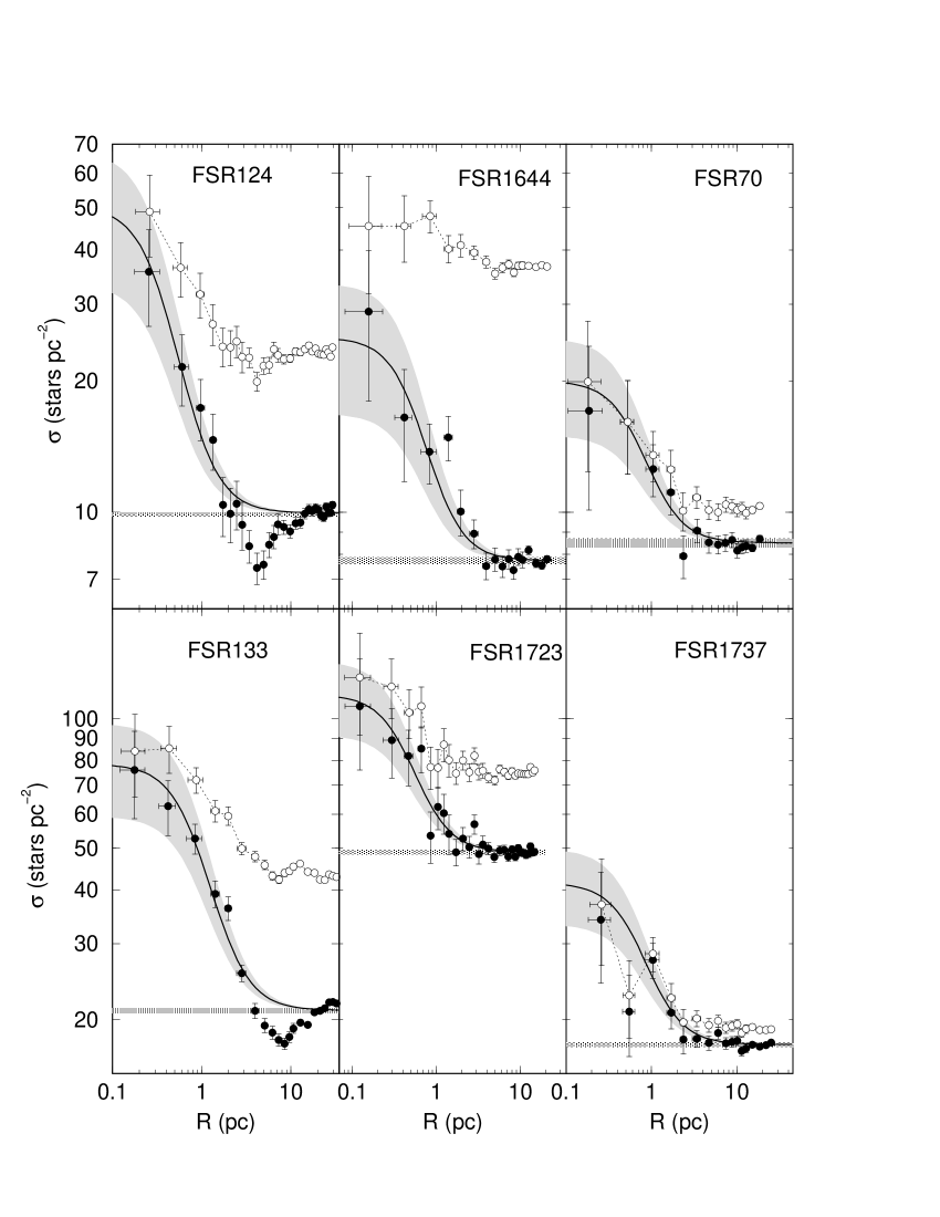
Figure 6: Stellar RDPs (filled circles) of the confirmed star clusters built with colour-magnitude photometry. Solid line: best-fit King profile. Horizontal shaded region: offset field stellar background level. Gray regions: $1\sigma$ King fit uncertainty. RDPs built with the observed photometry (empty circles) are shown for comparison. Absolute scale is used.

The resulting radial profiles of the 6 confirmed star clusters are given in Fig. 6. Besides the RDPs resulting from the colour-magnitude filters, we also show, for illustrative purposes, those produced with the observed (raw) photometry. Minimisation of non-cluster stars by the colour-magnitude filter resulted in RDPs with a significantly higher contrast with the background, especially for FSR1644, FSR124 and FSR 133. As expected for star clusters, the adopted King-like function describes well the RDPs throughout the full radii range, within uncertainties. $\sigma_{0}$ and the core radius ($\rm R_{C}$) are derived from the RDP fit, while $\sigma_{bg}$ is measured in the respective comparison field. These values are given in Table 4, and the best-fit solutions are superimposed on the colour-magnitude filtered RDPs (Fig. 6). Because of the 2MASS photometric limit, which in most cases corresponds to a cutoff for stars brighter than $\mbox{$\rm J$}\approx 16$, $\sigma_{0}$ should be taken as a lower limit to the actual central number-density.

The intrinsic contrast of a cluster RDP with the background which, in turn, is related to the difficulty of detection, can be quantified by the density contrast parameter $\delta_{c}=1+\sigma_{0}/\sigma_{bg}$ (col. 5 of Table 4). Interestingly, the objects projected not close to the Galactic centre, FSR 124, FSR 133 and FSR 1644, with $|\Delta\ell|\ga 45^{\circ}$, have $\delta_{c}\ga 3.3$, while the more central ones have $\delta_{c}\approx 2$. As a caveat we note that since $\delta_{c}$ is measured in colour-magnitude filtered RDPs, it does not necessarily correspond to the visual contrast produced in optical/IR images. The values of $\delta_{c}$ quoted in Table 4 are larger than the observed ones, as can be clearly seen in the observed RDPs (Fig. 6).

Table 4: Structural parameters measured in the RDPs built with colour-magnitude filtered photometry

		RDP
Cluster	$1\arcmin$	$\sigma_{bg}$	$\sigma_{0}$	$\delta_{c}$	$\rm R_{C}$	$\rm R_{lim}$
	(pc)	$\rm(stars\,pc^{-2})$	$\rm(stars\,pc^{-2})$		(pc)	(pc)
(1)	(2)	(3)	(4)	(5)	(6)	(7)
FSR 70	0.658	$9.6\pm 0.1$	$9.9\pm 4.4$	$2.0\pm 0.5$	$0.7\pm 0.2$	$3.3\pm 0.6$
FSR 124	0.749	$10.0\pm 0.1$	$40.4\pm 16.9$	$5.1\pm 1.7$	$0.4\pm 0.1$	$4.0\pm 1.0$
FSR 133	0.561	$21.0\pm 0.1$	$57.4\pm 19.0$	$3.7\pm 0.9$	$0.9\pm 0.2$	$4.4\pm 0.4$
Harvard 8,Cr 268†	0.554	$7.7\pm 0.1$	$17.4\pm 8.3$	$3.3\pm 1.0$	$0.6\pm 0.2$	$3.7\pm 0.3$
ESO 275SC1‡	0.365	$49.0\pm 0.3$	$64.6\pm 21.9$	$2.3\pm 0.4$	$0.5\pm 0.1$	$3.6\pm 0.6$
FSR 1737	0.800	$12.2\pm 0.1$	$16.6\pm 5.6$	$2.4\pm 0.2$	$0.8\pm 0.2$	$5.0\pm 0.3$

• $(\dagger)$: FSR 1644; $(\ddagger)$: FSR 1723. Col. 2: arcmin to parsec scale. To minimise degrees of freedom in RDP fits with the King-like profile (see text), $\sigma_{bg}$ was kept fixed (measured in the respective comparison fields) while $\sigma_{0}$ and $\rm R_{C}$ were allowed to vary. Col. 5: cluster/background density contrast ($\delta_{c}=1+\sigma_{0}/\sigma_{bg}$), measured in colour-magnitude filtered RDPs.

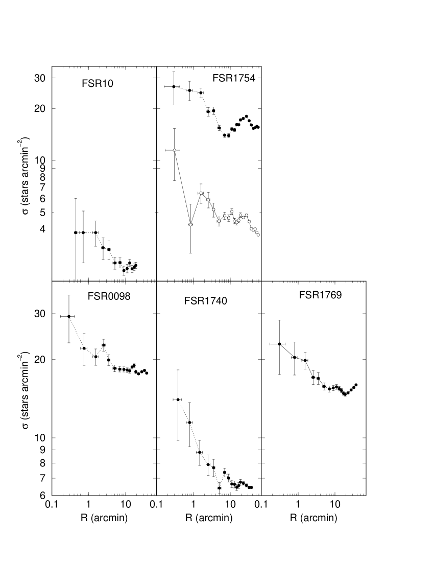
Figure 7: RDPs of the uncertain cases, in angular units. FSR 1754 has two RDPs corresponding to the red (black circles) and blue (empty circles) sequences seen in the decontaminated CMD (Fig. 3). The ”bump” at $\rm R\sim 30\arcmin$ in the RDP of FSR 1754 is produced by the OC NGC 6318.

Figure 8: RDPs of the possible field fluctuations, in angular units. They are narrower than the RDPs of the cluster-like (Fig. 6 and uncertain cases.

We also provide in col. 7 of Table 4 the cluster limiting radius and uncertainty, which are estimated by comparing the RDP (taking into account fluctuations) with the background level. $\rm R_{lim}$ corresponds to the distance from the cluster centre where RDP and background become statistically indistinguishable. For practical purposes, most of the cluster stars are contained within $\rm R_{lim}$. The limiting radius should not be mistaken for the tidal radius; the latter values are usually derived from King (or other analytical functions) fits to RDPs, which depend on wide surrounding fields and as small as possible Poisson errors (e.g. Bonatto & Bica 2007b). In contrast, $\rm R_{lim}$ comes from a visual comparison of the RDP and background level.

The empirical determination of a cluster-limiting radius depends on the relative levels of RDP and background (and respective fluctuations). Thus, dynamical evolution may indirectly affect the measurement of the limiting radius. Since mass segregation preferentially drives low-mass stars to the outer parts of clusters, the cluster/background contrast in these regions tends to lower as clusters age. As an observational consequence, smaller values of limiting radii should be measured, especially for clusters in dense fields. However, simulations of King-like OCs (Bonatto & Bica 2007b) show that, provided not exceedingly high, background levels may produce limiting radii underestimated by about 10–20%. The core radius, on the other hand, is almost insensitive to background levels (Bonatto & Bica 2007b). This occurs because $\rm R_{C}$ results from fitting the King-like profile to a distribution of RDP points, which minimises background effects.

The RDPs of the cases with uncertain CMD morphology are shown in Fig. 7. Except for FSR 10, which suffers from low-number statistics, the remaining RDPs suggest the presence of a star cluster.

Finally, in Fig. 8 we show the RDPs of the remaining targets. A narrow excess in the stellar density profile near the centre is present in all cases, but they are quite different from a King-like profile (e.g. Fig. 6).

5 Discussion

Following the photometric (Sect. 3) and RDP (Sect. 4) analyses, the 20 FSR overdensity/star cluster candidates dealt with in this paper can be split into the three distinct groups discussed below.

5.1 Star clusters

Objects in the first group have well-defined decontaminated CMD sequences (Figs. 1 and 2) with relatively high values of the parameter $\rm N_{1\sigma}$, both considering magnitude bins (Table 2) and the integrated one (Table 3), as well as King-like RDPs (Fig. 6). In most cases, the statistical significance of the decontaminated number of probable member stars, in individual magnitude bins, is $\ga 3\sigma$ with respect to fluctuations in the observed number of stars. Astrophysical parameters (age, distance, reddening, core and limiting radii) could be measured for these clusters. They are FSR 70, FSR 124, FSR 133, FSR 1644, FSR 1723 and FSR 1737. The average value of $\rm N_{1\sigma}$ is $\langle\mbox{$\rm N_{1\sigma}$}\rangle=6.2\pm 1.7$.

FSR 70: The decontaminated CMD ($\mbox{$\rm N_{1\sigma}$}=5.5$) is typical of an old cluster. In Fig. 2 we tentatively applied the 5 Gyr isochrone, which resulted in a distance from the Sun of $\mbox{$\rm d_{\odot}$}\approx 2.3$ kpc, and the Galactocentric distance $\mbox{$\rm R_{GC}$}\approx 5.3$ kpc. The RDP, with a density contrast $\delta_{c}\approx 2$, produced the structural parameters $\mbox{$\rm R_{C}$}\approx 0.7$ pc and $\mbox{$\rm R_{lim}$}\approx 3.3$ pc. Within uncertainties, the present $\rm R_{C}$ value agrees with that computed by Froebrich, Scholz & Raftery (2007) (Table 1).

FSR 124: The presence of an intermediate-age OC was already suggested by the observed CMD. With $\mbox{$\rm N_{1\sigma}$}=5.5$ in the decontaminated CMD, we derived the age $\approx 1$ Gyr, $\mbox{$\rm d_{\odot}$}\approx 2.6$ kpc and $\mbox{$\rm R_{GC}$}\approx 5.7$ kpc. From the highly contrasted RDP ($\delta_{c}\approx 5$) we derived $\mbox{$\rm R_{C}$}\approx 0.4$ pc and $\mbox{$\rm R_{lim}$}\approx 4.0$ pc. In this case our value of $\rm R_{C}$ is $\sim 1/3$ that in Froebrich, Scholz & Raftery (2007).

FSR 133: This OC presents the highest reddening value ($\mbox{$\rm A_{V}$}\approx 6$) among the present sample. It appears to be the most populous as well, with the decontaminated $\mbox{$\rm N_{1\sigma}$}\approx 10$. We found the age $\approx 550$ Myr, $\mbox{$\rm d_{\odot}$}\approx 1.9$ kpc and $\mbox{$\rm R_{GC}$}\approx 6.2$ kpc. From the RDP ($\delta_{c}\approx 4$) we derived $\mbox{$\rm R_{C}$}\approx 0.9$ pc ($\sim 1/2$ that in Froebrich, Scholz & Raftery 2007) and $\mbox{$\rm R_{lim}$}\approx 4.4$ pc.

Harvard 8, Cr 268 = FSR 1644: The decontamination ($\mbox{$\rm N_{1\sigma}$}=4.9$) was essential to uncover this OC with the age $\approx 550$ Myr, at $\mbox{$\rm d_{\odot}$}\approx 1.9$ kpc and $\mbox{$\rm R_{GC}$}\approx 6.3$ kpc. From the RDP ($\delta_{c}\approx 3.3$) we derived $\mbox{$\rm R_{C}$}\approx 0.6$ pc ($\sim 1/2$ that in Froebrich, Scholz & Raftery 2007) and $\mbox{$\rm R_{lim}$}\approx 3.7$ pc. WEBDA provides for this optical cluster under the designation Cr 268, $\mbox{$\rm E(B-V)$}=0.31$, $\mbox{$\rm d_{\odot}$}=1.96$ kpc and the age 0.57 Gyr, in excellent agreement with the present work (Table 3).

ESO 275SC1 = FSR 1723: An OC of age $\approx 0.8$ Gyr, at $\mbox{$\rm d_{\odot}$}\approx 1.3$ kpc and $\mbox{$\rm R_{GC}$}\approx 6.1$ kpc, clearly stands out both in the observed and decontaminated ($\mbox{$\rm N_{1\sigma}$}=5.9$) CMDs, which presents the lowest reddening ($\mbox{$\rm A_{V}$}\approx 0.1$) among the sample. The King-like RDP ($\delta_{c}\approx 2.3$) is characterised by $\mbox{$\rm R_{C}$}\approx 0.5$ pc (similar to that in Froebrich, Scholz & Raftery 2007) and $\mbox{$\rm R_{lim}$}\approx 3.6$ pc.

FSR 1737: Another case of an old OC whose decontaminated CMD ($\mbox{$\rm N_{1\sigma}$}=5.6$) suggests an age of 5 Gyr, or older. In the case of 5 Gyr, we estimated $\mbox{$\rm d_{\odot}$}\approx 2.8$ kpc and $\mbox{$\rm R_{GC}$}\approx 4.7$ kpc. Its RDP ($\delta_{c}\approx 2.4$) implies $\mbox{$\rm R_{C}$}\approx 0.8$ pc ($\sim 1/2$ that in Froebrich, Scholz & Raftery 2007) and $\mbox{$\rm R_{lim}$}\approx 5.0$ pc.

5.2 Uncertain cases

In general, targets of the second group have less defined decontaminated CMD sequences than those in the first group, which is consistent with the lower-level of the $\rm N_{1\sigma}$ parameter in magnitude bins, which reaches a statistical significance of $\sim 2\sigma$; however, their integrated $\rm N_{1\sigma}$ are, on average, of the same order ($\langle\mbox{$\rm N_{1\sigma}$}\rangle=6.1\pm 1.8$). They are FSR 10, FSR 98, FSR 1740, FSR 1769 and FSR 1754. Cluster sequences are suggested by the decontaminated CMDs (Fig. 3), e.g. giant clump and the top of the MS. RDPs of the objects in this group (Fig. 7) also suggest star clusters, although the large error bars of FSR 10 reflect the low-number statistics.

FSR 1754 is an interesting case whose decontaminated CMD presents two sequences, a blue one with $\mbox{$\rm N_{1\sigma}$}=5.5$ and a more populous red one with $\mbox{$\rm N_{1\sigma}$}=9.8$. The former may be from an intermediate-age cluster (IAC), while the latter might correspond to an old cluster. RDPs extracted from both sequences separately (Fig. 7) also suggest star clusters. We point out that the field of FSR 1754 contains the OC NGC 6318, at $\approx 26\arcmin$ from the centre (WEBDA), which can be seen in the RDP of FSR 1754 as a ”bump” on the wing (Fig. 7).

Decontaminated CMDs and RDPs taken together suggest that the above objects might be old clusters which require deeper observations. FSR 10, on the other hand, may be an IAC. Deeper photometry is essential in most cases, especially for old OCs for which the TO is close to the 2MASS limiting magnitude. In this context, we would recommend also that the same applies to FSR 70 and FSR 1737 (Sect. 5.1), for a better definition of the TO region and, consequently, the age and distance from the Sun.

5.3 Possible field fluctuations

Decontaminated CMDs of this group have $\rm N_{1\sigma}$-values significantly lower than those of the star clusters (Sect. 5.1) and uncertain cases (Sect. 5.2). Indeed, the average integrated $\rm N_{1\sigma}$ is $\langle\mbox{$\rm N_{1\sigma}$}\rangle=3.5\pm 0.5$, while the statistical significance of the probable member stars in individual magnitude bins is below the $2\sigma$ level. The fact that they have $\mbox{$\rm N_{1\sigma}$}\sim 3$ is consistent with the method employed by Froebrich, Scholz & Raftery (2007) to detect overdensities. However, in most cases the RDP excess is very narrow, restricted to the first bins, quite different from a King-like profile (e.g. Fig. 6).

The third group has essentially featureless (observed and decontaminated) CMDs, and RDPs with important deviations from cluster-like profiles. They appear to be $\sim 3\sigma$ fluctuations of the dense stellar field over which these objects are projected.

5.4 Relations among astrophysical parameters

To put the present FSR OCs into perspective we compare in Fig. 9 their astrophysical parameters with those measured in OCs in different environments. We consider (i) a sample of bright nearby OCs (Bonatto & Bica 2005), including the two young OCs NGC 6611 (Bonatto, Santos Jr. & Bica 2006) and NGC 4755 (Bonatto et al. 2006b), (ii) OCs projected against the central parts of the Galaxy (Bonatto & Bica 2007b), and (iii) the recently analysed OCs FSR 1744, FSR 89 and FSR 31 (Bonatto & Bica 2007a), which are similarly projected against the central parts of the Galaxy as the present FSR cluster sample (iv). OCs in sample (i) have ages in the range $\rm 70\,Myr\la age\la 7\,Gyr$ and Galactocentric distances in the range $\rm 5.8\la\mbox{$\rm R_{GC}$}(kpc)\la 8.1$. NGC 6611 has $\rm age\approx 1.3$ Myr and $\mbox{$\rm R_{GC}$}=5.5$ kpc, and NGC 4755 has $\rm age\approx 14$ Myr and $\mbox{$\rm R_{GC}$}=6.4$ kpc. Sample (ii) OCs are characterised by $\rm 600\,Myr\la age\la 1.3\,Gyr$ and $\rm 5.6\la\mbox{$\rm R_{GC}$}(kpc)\la 6.3$. FSR 1744, FSR 89 and FSR 31 are Gyr-class OCs at $\rm 4.0\la\mbox{$\rm R_{GC}$}(kpc)\la 5.6$.

Core and limiting radii of the OCs in samples (i) and (ii) are almost linearly related by $\mbox{$\rm R_{lim}$}=(8.9\pm 0.3)\times R_{\rm core}^{(1.0\pm 0.1)}$ (panel (a)), which suggests a similar scaling in both kinds of radii, in the sense that on average, larger clusters tend to have larger cores, at least for $\rm 0.5\la\mbox{$\rm R_{C}$}(pc)\la 1.5$ and $\rm 5\la\mbox{$\rm R_{lim}$}(pc)\la 15$. Linear relations between OC core and limiting radii were also found by Nilakshi, Pandey & Mohan (2002), Sharma et al. (2006), and Maciejewski & Niedzielski (2007). However, about $2/3$ of the OCs in samples (iii) and (iv) do not follow that relation, which suggests that they are either intrinsically small or have suffered important evaporation effects (see below). The core and limiting radii of FSR 124 and FSR 1723 are consistent with the relation at the $1\sigma$ level.

A dependence of OC size on Galactocentric distance is implied by panel (b), as previously suggested by Lyngå (1982) and Tadross et al. (2002). In this context, the limiting radii of the present FSR OCs are roughly consistent with their positions in the Galaxy, especially FSR 1737, the innermost OC of the sample. Since core and limiting radii appear to be linearly related (panel a), a similar conclusion applies to the core radius. Part of this relation may be primordial, in the sense that the higher density of molecular gas in central Galactic regions may have produced clusters with smaller core radii, as suggested by van den Bergh, Morbey & Pazder (1991) to explain the increase of GC radii with Galactocentric distance. In addition, there is the possibility that the core size may also be a function of the binary fraction and its evolution with age, so that loss of stars may not be the only process to determine sizes.

Core and limiting radii are compared with cluster age in panels (c) and (d), respectively. This relationship is intimately related to cluster survival/dissociation rates. Both kinds of radii present a similar dependence on age, in which part of the clusters expand with time, while some seem to shrink. The bifurcation occurs at $\rm age\sim 1$ Gyr. Except for FSR 133 (and perhaps, FSR 1737), the remaining FSR OCs have core radii typical of the small OCs in the lower branch; the limiting radii, on the other hand, locate in the lower branch.

With respect to the astrophysical parameters discussed above, the present FSR star clusters can be taken as similar objects as FSR 1744, FSR 89 and FSR 31 (Bonatto & Bica 2007a). In that study we interpreted the relatively small radii of the latter OCs as resulting from the enhanced dynamical evolution combined to low-contrast. Effects such as the tidal pull of the Galactic bulge, frequency of collisions with giant molecular clouds and spiral arms, low-mass star evaporation and ejection, which are more important in the inner Galaxy, tend to accelerate the dynamical evolution, especially of low-mass star clusters (Bonatto & Bica 2007a, and references therein). As a result, the mass of the OCs decreases with time.

One consequence of the mass segregation associated to the dynamical evolution is the large-scale transfer of low-mass stars towards the external parts, which reduces the surface brightness at large radii. When projected against the central parts of the Galaxy, such star clusters (as well as the poorly-populated ones) suffer from low-contrast effects, especially in the external parts. Bonatto & Bica (2007b) found that low contrast may underestimate the limiting radii of centrally projected OCs by about $10-20\%$. The core radii, on the other hand, are not affected. Thus, the small sizes of the present FSR clusters derived here appear to be related to dynamical effects.

Finally, in Fig. 10 we show the spatial distribution in the Galactic plane of the present FSR OCs, compared to that of the OCs in the WEBDA database. We consider the age ranges $\rm<0.4$ Gyr, $\rm 0.4\,Gyr-1$ Gyr and $\rm>1$ Gyr. FSR 31, FSR 89 and FSR 1744 are also shown. Old OCs are found preferentially outside the Solar circle, and the inner Galaxy contains few OCs so far detected. The interesting point here is whether inner Galaxy clusters cannot be observed because of strong absorption and crowding, or have been systematically dissolved by the different tidal effects combined (Bonatto & Bica 2007a, and references therein). In this context, the more OCs are identified (with their astrophysical parameters derived) in the central parts, the more constraints can be established to settle this issue.

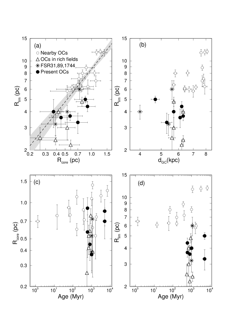
Figure 9: Relations involving astrophysical parameters of OCs. Empty circles: nearby OCs, including two young ones. Triangles: OCs projected on dense fields towards the centre. Stars: the similar OCs FSR 31, FSR 89 and FSR 1744. Black circles: the OCs dealt with in this work.

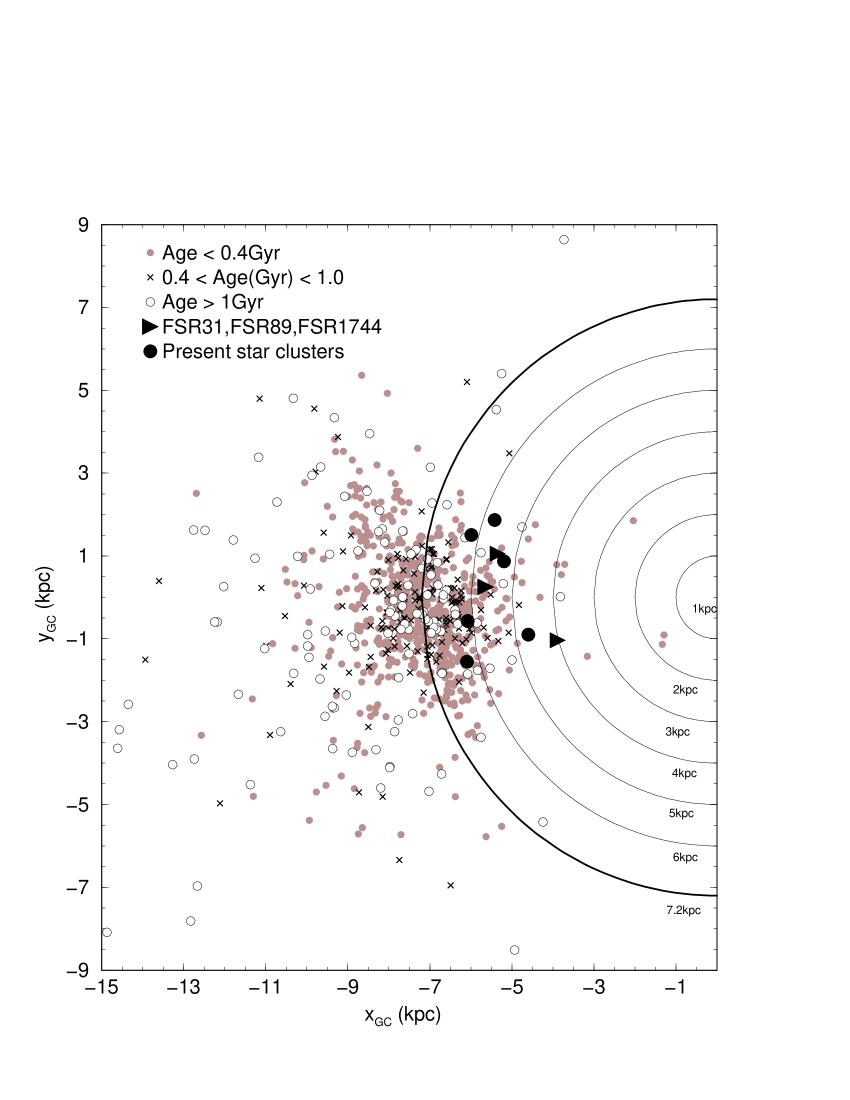
Figure 10: Spatial distribution of the present star clusters (black circles) compared to the WEBDA OCs with ages younger than 0.4 Gyr (gray circles), $\rm 0.4<age<1.0$ Gyr (’x’), and older than 1 Gyr (empty circles). For comparison we also show the position of the similar OCs FSR 31, FSR 89 and FSR 1744 (black triangles).

6 Summary and conclusions

The discovery of new star clusters in the Galaxy, and the derivation of their astrophysical parameters, provide important information that, in turn, can be used in a variety of other studies related to the star formation and evolution processes, dynamics of N-body systems, disruption time scales, the geometry of the Galaxy, among others.

In this work we selected a sample of star cluster candidates projected nearly towards the dense stellar field of the bulge ($|\Delta\ell|\la 60^{\circ}$, $|\Delta\,b|\la 20^{\circ}$), from the catalogue of Froebrich, Scholz & Raftery (2007). They classified them as probable and possible star clusters, with quality flag ’0’ or ’1’. The resulting 20 targets were analysed with 2MASS photometry by means of field-star decontaminated colour-magnitude diagrams, colour-magnitude filters and stellar radial density profiles.

Of the 20 overdensities, 6 resulted with cluster-like CMDs and King-like RDPs (among these are the already catalogued open clusters Harvard 8=Cr 268, and ESO 275SC1). These are star clusters with ages in the range 0.6 Gyr to $\sim 5$ Gyr, at distances from the Sun $\rm 1.3\la\mbox{$\rm d_{\odot}$}(kpc)\la 2.8$, and Galactocentric distances $\rm 4.7\la\mbox{$\rm R_{GC}$}(kpc)\la 6.3$. Five others have CMDs and RDPs that suggest old star clusters, but they require deeper photometry to establish their nature. Some of the uncertain cases might be globular clusters, considering the high value of the field-star decontaminated CMD density parameter $\rm N_{1\sigma}$ and the similarity with the bulge CMD. The remaining 9 overdensities are likely fluctuations of the associated dense stellar field.

Considering the above numbers, the fraction of overdensities that turned out to be star cluster ($f_{SC}$) can be put in the range $30\%\la f_{SC}\la 55\%$. The upper limit agrees with the $f_{SC}\approx 50\%$ estimated by Froebrich, Scholz & Raftery (2007).

Systematic surveys such as that of Froebrich, Scholz & Raftery (2007) are important to detect new star cluster candidates throughout the Galaxy. Nevertheless, works like the present one, that rely upon field-star decontaminated CMDs and stellar radial profiles, are fundamental to probe the nature of such candidates, especially those projected against dense stellar fields.

References

- van den Bergh & Hagen (1975) van den Bergh, S. & Hagen, G.L., 1975, AJ, 80, 11
- van den Bergh & McClure (1980) van den Bergh, S. & McLure, R.D. 1980, A&A, 88, 360
- van den Bergh, Morbey & Pazder (1991) van den Bergh, S., Morbey, C. & Pazder, J. 1991, ApJ, 375, 594
- Bergond, Leon & Guilbert (2001) Bergond, G., Leon, S. & Guilbert, J. 2001, A&A, 377, 462
- Bessel & Brett (1988) Bessel, M.S. & Brett, J.M. 1988, PASP, 100, 1134
- Bica et al. (2006) Bica, E., Bonatto, C., Barbuy, B. & Ortolani, S. 2006, A&A, 450, 105
- Bica et al. (2007) Bica, E., Bonatto, C., Ortolani, S. & Barbuy, B. 2007, A&A, 472, 483
- Bonatto, Bica & Girardi (2004) Bonatto, C., Bica, E. & Girardi, L. 2004, A&A, 415, 571
- Bonatto, Bica & Santos Jr. (2005) Bonatto, C., Bica, E. & Santos Jr., J.F.C. 2005, A&A, 433, 917
- Bonatto & Bica (2005) Bonatto, C. & Bica, E. 2005, A&A, 437, 483
- Bonatto et al. (2006a) Bonatto, C., Kerber, L.O., Bica, E. & Santiago, B.X. 2006a, A&A, 446, 121
- Bonatto et al. (2006b) Bonatto, C., Bica, E., Ortolani, S. & Barbuy, B. 2006b, A&A, 453, 121
- Bonatto, Santos Jr. & Bica (2006) Bonatto, C., Santos Jr., J.F.C. & Bica, E. 2006, A&A, 445, 567
- Bonatto & Bica (2007a) Bonatto, C. & Bica, E. 2007a, A&A, 473, 445
- Bonatto & Bica (2007b) Bonatto, C. & Bica, E. 2007b, MNRAS, 377, 1301
- Bonatto et al. (2007) Bonatto, C., Bica, E., Ortolani, S. & Barbuy, B. 2007, MNRAS, 381, L45
- Dutra, Santiago & Bica (2002) Dutra, C.M., Santiago, B.X. & Bica, E. 2002, A&A, 383, 219
- Elson, Fall & Freeman (1987) Elson, R.A.W., Fall, S.M. & Freeman, K.C. 1987, ApJ, 323, 54
- Froebrich, Meusinger & Scholz (2007) Froebrich, D., Meusinger, H. & Scholz, A. 2007, MNRAS, 377, L54
- Froebrich, Scholz & Raftery (2007) Froebrich, D., Scholz, A. & Raftery, C.L. 2007, MNRAS, 374, 399
- Froebrich, Meusinger & Davis (2007) Froebrich, D., Meusinger, H. & Davis, C.J. 2007, MNRAS, in press (astro-ph:0710-2030)
- Gieles et al. (2006) Gieles, M., Portegies Zwart, S.F., Baumgardt, H., Athanassoula, E., Lamers, H.J.G.L.M. Sipior, M. & Leenaarts, J. 2006, MNRAS, 371, 793
- Girardi et al. (2002) Girardi, L., Bertelli, G., Bressan, A., et al. 2002, A&A, 391, 195
- Hurley & Tout (1998) Hurley, J. & Tout, A.A. 1998, MNRAS, 300, 977
- Kerber et al. (2002) Kerber, L.O., Santiago, B.X., Castro, R. & Valls-Gabaud, D. 2002, A&A, 390, 121
- Kharchenko et al. (2005) Kharchenko, N.V., Piskunov, A.E., Röser, S., Schilbach, E. & Scholz, R.-D. 2005, A&A, 438, 1163
- King (1962) King, I. 1962, AJ, 67, 471
- King (1966) King, I. 1966, AJ, 71, 64
- Lamers et al. (2005) Lamers, H.J.G.L.M., Gieles, M., Bastian, N., Baumgardt, H., Kharchenko, N.V. & Portegies Zwart, S. 2005, A&A, 441, 117
- Lauberts (1982) Lauberts, A., 1982, in ESO/Uppsala Survey of the ESO (B) Atlas, ESO:Garching
- Lyngå (1982) Lyngå, G. 1982, A&A, 109, 213
- Maciejewski & Niedzielski (2007) Maciejewski, G. & Niedzielski, A. 2007, A&A, 467, 1065
- Mermilliod & Paunzen (2003) Mermilliod, J.C. & Paunzen, E. 2003, A&A, 410, 511
- Nilakshi, Pandey & Mohan (2002) Nilakshi, S.R., Pandey, A.K. & Mohan, V. 2002, A&A, 383, 153
- Pavani & Bica (2007) Pavani, D.N. & Bica, E. 2007, MNRAS, 468, 139
- Piskunov et al. (2007) Piskunov, A.E., Schilbach, E., Kharchenko, N.V., Röser, S. & Scholz, R.-D. 2007, A&A, 468, 151
- Portegies Zwart et al. (2002) Portegies Zwart, S.F., Makino, J., McMillan, S.L.W. & Hut, P. 2002, ApJ, 565, 265
- Sharma et al. (2006) Sharma, S., Pandey, A. K., Ogura, K., Mito, H., Tarusawa, K. & Sagar, R. 2006, AJ, 132, 1669
- Tadross et al. (2002) Tadross, A.L., Werner, P., Osman, A. & Marie, M. 2002, NewAst, 7, 553
- Willman et al. (2005) Willman, B., Blanton, M.R., West, A.A. et al. 2005, AJ, 129, 2692
- Wilson (1975) Wilson, C.P. 1975, AJ, 80, 175