The Magic Angle “Mystery” in Electron Energy Loss Spectra: Relativistic and Dielectric Corrections

Abstract

Recently it has been demonstrated that a careful treatment of both longitudinal and transverse matrix elements in electron energy loss spectra can explain the mystery of relativistic effects on the magic angle. Here we show that there is an additional correction of order $(Z\alpha)^{2}$ where $Z$ is the atomic number and $\alpha$ the fine structure constant, which is not necessarily small for heavy elements. Moreover, we suggest that macroscopic electrodynamic effects can give further corrections which can break the sample-independence of the magic angle.

I Introduction

The title of this article is in reference to a recent work by Jouffrey et al. Jouffrey et al. (2004) with the title “The Magic Angle: A Solved Mystery.” The magic angle in electron energy loss spectroscopy (EELS) is a special value of the microscope collection-angle $\alpha_{c}$ at which the measured spectrum “magically” becomes independent of the angle between the incoming beam and the sample “$c$-axis.” The mystery, in the context of 200 keV electron microscopy, is that standard semi-relativistic quantum theory yields a ratio of the magic angle $\theta_{M}$ to “characteristic angle” $\theta_{E}$ of more than twice the observed Daniels et al. (2003) value. Unfortunately, time Paxton et al. (2000) and again,Daniels et al. (2003); Hebert et al. (2004) the theoretical justification of the factor of two turned out to be an errant factor of two elsewhere in the calculation. A key contribution of Jouffrey et al. was the observation that relativistic “transverse” effects, when properly included in the theory, naturally give a factor of two correction to the non-relativistic magic angle. Here we show that there are yet additional corrections to the theory which can even break the sample independence of the magic angle.

As in Ref. [Jouffrey et al., 2004], we consider here the problem of a relativistic probe electron scattering off of a macroscopic condensed matter sample. Similar problems have been solved long ago using both semi-classical Moller (1932) and fully quantum-mechanical approachs.Bethe (1930); Fano (1956, 1963) Indeed, the fully quantum-mechanical, relativistic case of scattering two plane-wave electrons has long been a textbook problem.Heitler (1954); Peskin and Schroeder (1995) This classic problem was revived recently in the works of Jouffrey et al. Jouffrey et al. (2004) and of Schattschneider et al.,Schattschneider et al. (2005) in which a “flaw” in the standard theory is pointed out. The flaw is the approximation that the so-called “longitudinal” and “transverse” matrix elements for the scattering process may be summed incoherently, as argued by Fano in a seminal paper.Fano (1956) In fact, this approximation is only valid when the sample under consideration posseses certain symmetries. In a later review article,Fano (1963) Fano states this condition explicitly; namely that his original formula for the cross-section is only applicable to systems of cubic symmetry. However, this caveat, seems to have been generally ignored, and hence turns out to be the source of the magic angle “mystery”.Jouffrey et al. (2004) Jouffrey et al., and later Schattschneider et al., showed that if one correctly sums and squares the transition matrix elements then, in the dipole approximation, one finds the magic angle corrected by a factor of two.

Our aim here is to examine the theory in more detail in order to derive both relativistic and material-dependent corrections to the magic angle. In Section II we consider relativistic electron scattering within the formalism of quantum electrodynamics (QED). Working the Coulomb gauge, we show that one can almost reproduce the results of Jouffrey et al. and the theory of Schattschneider et al., apart from a simple correction term of order ${\hbar\omega}/{mc^{2}}$, which is not always negligible. Here $\hbar\omega$ is the energy lost by the probe and $mc^{2}$ is the rest energy of an electron. In Section III we suggest the possibility of incorporating macroscopic electrodynamic effects into the theory, which can break the symmetry of sample independence of the magic angle.

II Coulomb Gauge Calculation

An appealing aspect of the formalism of Schattschneider et al. is its simplicity. Their approach is similar to the semi-classical approach of Møller,Moller (1932) but with the added simplification of working with a probe and sample described by the Schrödinger equation, rather than the Dirac equation. They also find that the theory is simplified by choosing to work in the Lorentz gauge. Unfortunately, however, the theory of Møller is somewhat ad hoc in that a classical calculation in the Lorentz gauge is modified by replacing the product of two classical charge densities by the product of four different wavefunctions in order to obtain the transition matrix element. For the Møller case this procedure is justified a posteriori by the fact that it reproduces the correct result, but is only rigorously justified by appealing to the method of second quantization.Heitler (1954) Møller’s proceedure is physically reasonable a priori, because Møller was interested in the scattering of electrons in vacuum. However, the theory of Schattschneider et al., which largely mimics Møller’s theory, is less physically reasonable a priori, since the electrons are not scattering in vacuum, but are inside a solid which can screen the electrons. Nevertheless, since the discrepancy is small, the Schattschneider et al., theory is justified a posteriori to a lesser extent by experiment.Daniels et al. (2003) We thus refer to the theory of Schattschneider et al. as a “vacuum-relativisitic theory.” Consequently, in an effort to account for the discrepancy with experiment, we feel that it is useful to rederive the results of Jouffrey et al. from a more fundamental starting point.

It is easy to see that the theory of Schattschneider et al. is not formally exact, though for many materials the error in the vacuum relativistic limit is negligible. In fact, the discrepancy can be easily explained via single-particle quantum mechanics: although Schattschneider et al. work explicitly in the Lorentz gauge, they also make the assumption that the momentum and the vector potential commute,

$${\bm{p}}\cdot{\bm{A}({\bm{r}})}\stackrel{{\scriptstyle?}}{{=}}{\bm{A}({\bm{r}})}\cdot{\bm{p}}.$$ (1)

Of course, this commutation relation is only exact in the Coulomb gauge. In the end, however, the error in this approximation only effects the final results (e.g., matrix elements) by a correction of order $\hbar\omega/mc^{2}$ compared to unity, where $\hbar\omega$ is the energy lost by the probe. Since $\hbar\omega/mc^{2}$ is at most $(Z\alpha)^{2}$ for deep-core energy loss, the effect is usually negligible, except of course, for very heavy atoms. To see how corrections such as the above enter into the theory, and further to determine whether or not such corrections are meaningful or simply artifacts of the various approximations used in the theory of Schattschneider et al., we find it useful to present a fully quantum-mechanical, relativistic many-body treatment along the lines of Fano,Fano (1963) but without any assumption of symmetry of the sample. Our treatment is at least as general as that of Schattschneider et al. as far as the symmetry of the sample is concerned. Thus going beyond the formulations of Schattschneider et al. and Møller, we take as our starting point the many-particle QED Hamiltonian. We then show that in a single-particle approximation the theory yields the result of Schattschneider et al. together with the correction mentioned above.

Our starting point therefore is the Hamiltonian in Coulomb gauge Heitler (1954)

$$H=H_{\textrm{el}}+H_{\textrm{int}}+H_{\textrm{rad}}\;,$$ (2)

where the Hamiltonian has been split into three parts: i) the unperturbed electron part

$$H_{\textrm{el}}=\int d^{3}x\,\psi^{\dagger}({\bm{x}})\left(c{\bm{\alpha}}\cdot{\bm{p}}+{\bm{\beta}}mc^{2}\right)\psi({\bm{x}}),$$ (3)

where $\psi({\bm{x}})$ is the second-quantized Dirac field, ${\bm{\alpha}_{i}}$ and ${\bm{\beta}}$ are the usual Dirac matrices, $m$ is the electron mass, and $c$ is the speed of light;

ii) the unperturbed (transverse) radiation part

$$H_{\textrm{rad}}=\sum_{{\bm{k}}}\sum_{i=1}^{2}a^{\dagger}_{{\bm{k}},i}a_{{\bm{k}},i}\hbar\omega_{k},$$ (4)

where $a_{{\bm{k}},i}$ destroys a photon of momentum ${\bm{k}}$, polarization ${\bm{\epsilon}}_{{\bm{k}},i}$, and energy $\hbar\omega_{k}$; and

iii) the interaction part

$$H_{\textrm{int}} = +\ e\int d^{3}x\,\psi^{\dagger}({\bm{x}}){\bm{\alpha}}\cdot{\bm{A}({\bm{x}})}\psi({\bm{x}}),$$ (5)

$$+ \frac{e^{2}}{2}\int d^{3}xd^{3}y\frac{\psi^{\dagger}({\bm{x}})\psi^{\dagger}({\bm{y}})\psi({\bm{y}})\psi({\bm{x}})}{|{\bm{x}}-{\bm{y}}|},$$

where

$${\bm{A}}({\bm{x}})=\sum_{{\bm{k}},{i}}\sqrt{\frac{2\pi\hbar c^{2}}{V\omega_{k}}}\left(a_{{\bm{k}},{i}}{\bm{\epsilon}}_{{\bm{k}},i}e^{i{\bm{k}}\cdot{\bm{x}}}+a_{{\bm{k}},i}^{\dagger}{{{\bm{\epsilon}}}^{*}}_{{\bm{k}},i}e^{-i{\bm{k}}\cdot{\bm{x}}}\right),$$ (6)

$e=|e|$ is the charge of the proton, and $V$ is the system volume.

Let us next specialize to the case of a fixed number ($N+1$) of electrons where the ($N+1$)-th electron is singled out as the “fast probe” traveling with velocity ${\bm{v}_{0}}$, and the remaining $N$ electrons make up the sample. We also introduce a lattice or cluster of ion-cores (below we consider only elemental solids of atomic number $Z$ but the generalization to more complex systems is obvious) which is treated classically, and which gives rise to a potential $v_{\textrm{e-core}}({\bm{x}})=\sum_{i=1}^{N/Z}(-Ze^{2})/|{\bm{x}}-{\bm{R}_{i}}|$ as seen by the electrons. In this case our Hamiltonian becomes:

$$H = \left[c{\bm{\alpha}}\cdot({\bm{p}}+\frac{e}{c}{\bm{A}}({\bm{r}}))+{\bm{\beta}}mc^{2}\right]+v_{\textrm{e-core}}({\bm{r}})$$ (7)

$$+ \sum_{i=1}^{N}\left[c{\bm{\alpha}^{(i)}}\cdot({\bm{p}^{(i)}}+\frac{e}{c}{\bm{A}}({\bm{r}^{(i)}}))+{\bm{\beta}^{(i)}}mc^{2}\right]$$

$$+ e^{2}\sum_{i=1}^{N}\frac{1}{|{\bm{r}}-{\bm{r}^{(i)}}|}+\frac{e^{2}}{2}\sum_{1=i\neq j=1}^{N}\frac{1}{|{\bm{r}^{(i)}}-{\bm{r}^{(j)}}|}$$

$$+ \sum_{i=1}^{N}v_{\textrm{e-core}}({\bm{r}^{(i)}})+v_{\textrm{core-core}}+H_{\textrm{rad}}\;,$$

where the coordinates which are not labelled by an index refer to the probe electron. The interaction $v_{\textrm{core-core}}$ between ion cores is a constant and is henceforth dropped.

To proceed to a single-particle approximation for the sample, the interaction of the sample electrons among themselves and with the potential of the ion cores may be taken into account by introducing a single-particle self-consistent potential $v({\bm{x}})$ which includes both $v_{\textrm{e-core}}({\bm{x}})$ and exchange-correlation effects. The interaction of the probe electron with the effective single electron of the sample will be considered explicitly. The difference between this interaction and the actual interaction between the probe and sample can be accounted for by introducing another potential $v^{\prime}({\bm{x}})$ which is not necessarily the same as $v({\bm{x}})$; $v^{\prime}({\bm{x}})$ is, in theory, “closer” to the pure $v_{\textrm{e-core}}({\bm{x}})$ potential than $v({\bm{x}})$ though, in practice, this difference may not be of interest (see the Appendix for further explanation of this point). The potential $v^{\prime}({\bm{x}})$ leads to diffraction of the probe electron, which will not be considered in this paper in order to make contact with the theory of Schattschneider et al. It is also for this reason that we have introduced a single-particle picture of the sample, along with the fact that we want to apply this theory to real condensed matter systems in a practical way. The extension to the many-body case, in which the only single-body potential seen by the probe is due to the ion-cores, is given in the Appendix. Thus using the single-particle approximation for the sample,

$$H = \left[c{\bm{\alpha}}\cdot[{\bm{p}}+\frac{e}{c}{\bm{A}}({\bm{r}})]+{\bm{\beta}}mc^{2}\right]$$ (8)

$$+ \left[c{\bm{\alpha}_{s}}\cdot[{\bm{p}_{s}}+\frac{e}{c}{\bm{A}}({\bm{r}_{s}})]+{\bm{\beta}_{s}}mc^{2}\right]$$

$$+ v^{\prime}({\bm{r}})+e^{2}\frac{1}{|{\bm{r}}-{\bm{r}_{s}}|}+v({\bm{r}_{s}})+H_{\rm rad},$$

where the quantities labeled by the letter $s$ refer to the sample electron and the unlabeled quantites refer to the probe electron. In the remainder of this paper we set $v^{\prime}\to 0$, though the generalization of the theory to include diffraction is not expected to be difficult.

As it turns out,Fujiwara (1961) we may start from an effective Schrödinger treatment of both the sample and the probe rather than a Dirac treatment. The treatment of the probe by a “relativistically corrected” Schrödinger equation is standard practice Peng et al. (2004) in much of EELS theory, and is appropriate Fujiwara (1961) for modern microscope energies of interest here (e.g., a few hundred keV). The relativistic correction to the Schrödinger equation of the probe consists in simply replacing the mass of the probe $m$ by the relativistic mass $m^{\prime}=m\gamma$ where $\gamma=1/\sqrt{1-v_{0}^{2}/c^{2}}$. Moreover working with a Schrödinger equation treatment facilitates contact with the “vacuum-relativistic” magic-angle theory of Schattschneider et al. We will indicate later how the results change if we retain a full Dirac treatment of the electrons. Thus we may start with the Hamiltonian

$$H = \frac{[{\bm{p}}+({e}/{c}){\bm{A}}({\bm{r}})]^{2}}{2m^{\prime}}+\frac{[{\bm{p}_{s}}+({e}/{c}){\bm{A}}({\bm{r}_{s}})]^{2}}{2m}$$ (9)

$$+ v({\bm{r}_{s}})+\frac{e^{2}}{|{\bm{r}_{s}}-{\bm{r}}|}+H_{\textrm{rad}}$$

$$\equiv H_{0}+\frac{e}{m^{\prime}c}{\bm{p}}\cdot{\bm{A}}({\bm{r}})+\frac{e}{mc}{\bm{p}_{s}}\cdot{\bm{A}}({\bm{r}_{s}})$$

$$+ \frac{e^{2}}{|{\bm{r}_{s}}-{\bm{r}_{p}}|}+O(A^{2})\;.$$

In this theory the unperturbed states are then direct products of unperturbed sample electron states (which in calculations can be described, for example, by the computer code FEFF8,Ankudinov et al. (1998)) unperturbed probe electron states (plane-waves, ignoring diffraction), and the free (transverse) photon states. Also, from now on we ignore the interaction terms which are $O(A^{2})$. Thus our perturbation is

$$U=\frac{e^{2}}{|{\bm{r}}-{\bm{r}_{s}}|}+\frac{e}{m^{\prime}c}\,{\bm{p}}\cdot{\bm{A}}({\bm{r}})+\frac{e}{mc}\,{\bm{p}_{s}}\cdot{\bm{A}}({\bm{r}_{s}}),$$ (10)

and we are interested in matrix elements of

$$U+UG_{0}U+\ldots$$ (11)

where the one-particle Green’s function is

$$G_{0}(E)=\frac{1}{E-H_{0}+i\eta}$$ (12)

and $\eta$ is a postive infinitesimal. The matrix elements are taken between initial and final states (ordered as: probe, sample, photon)

$$|I\rangle=\left|k_{I}\right>\left|i\right>\left|0\right>\quad{\rm and}\quad|F\rangle=\left|k_{F}\right>\left|f\right>\left|0\right>\;.$$ (13)

To lowest order ($e^{2}$) there will be a “longitudinal” (instantaneous Coulomb) contribution to the matrix element, and a “transverse” (photon mediated) contribution, as illustrated in Fig. 1.

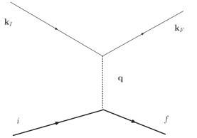
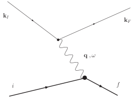
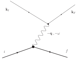
Figure 1: Feynman diagrams for the scattering process due to both the instantaneous Coulomb interaction (upper) and the transverse photon interaction (middle, lower). The solid lines labeled by momenta $\textbf{k}_{I}$ and $\textbf{k}_{F}$ represent the probe particle; thick solid lines labeled by the letters $i$ and $f$ represent the sample particle; the dashed line is the instantaneous Coulomb interaction; and the wiggly lines are transverse photons. Time flows to the right.

Instead of elaborating the details from standard perturbation theory, we simply write down the result for the matrix element

$$M = \frac{4\pi e^{2}}{V}\left[\frac{1}{q^{2}}\left<f\right|e^{i{\bm{q}}\cdot{\bm{r}_{s}}}\left|i\right>\right.$$ (14)

$$+ \left.\frac{1}{\omega^{2}-c^{2}q^{2}}\frac{k_{T}^{j}}{m^{\prime}}\left<f\right|\frac{p_{s}^{j}}{m}e^{i{\bm{q}}\cdot{\bm{r}_{s}}}\left|i\right>\right]\;,$$

where ${\bm{k}_{T}}$ (see Fig. 2) is the part of the initial (or final) momentum which is perpendicular to the momentum transfer $\hbar{\bm{q}}$. In the remainder of this paper we will choose our units such that $\hbar=1$.

$$k_{T}^{j}=\left(\delta_{lj}-\frac{q_{l}q_{j}}{q^{2}}\right)k_{F}^{l}=\left(\delta_{lj}-\frac{q_{l}q_{j}}{q^{2}}\right)k_{I}^{l}\;.$$ (15)

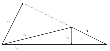
Figure 2: The relevant momenta: ${\bm{k}_{I}}$ is the initial momentum of the probe particle, ${\bm{k}_{F}}$ is the final momentum of the probe particle, ${\bm{q}}$ is the momentum transfer ${\bm{k}_{I}}-{\bm{k}_{F}}$ and ${\bm{k}_{T}}$ is the part of both the initial of final momenta which is perpendicular to the momentum transfer.

The result of Eq. (14) is easy to understand diagramatically. For example, to each wiggly line of momentum ${\bm{q}}$ and energy $\omega$ we may assign a value

$$\frac{1}{\omega-c|{\bm{q}}|}\left(\delta_{ij}-\frac{q_{i}q_{j}}{q^{2}}\right)\frac{2\pi c}{V|{\bm{q}}|}\;.$$ (16)

At this point we note that the relativistic many-body version of Eq. (14) can be obtained by making intuitively reasonable replacements such as ${\bm{p}}/{m}\to c{\bm{\alpha}}$, $e^{i{\bm{q}}\cdot{\bm{r}_{s}}}\to\sum_{i}e^{i{\bm{q}}\cdot{\bm{r}^{(i)}}}$. See the Appendix for further details.

Eq. (14) is equivalent to the matrix elements given by Fano in Eq. (12) of Ref. [Fano, 1963]. The cross-section given by Fano in Eq. (16) of Ref. [Fano, 1963], in which the matrix elements have been summed incoherently, is not generally correct and is the source of the magic angle “mystery”.Schattschneider et al. (2005)

Before continuing to the dipole approximation it is useful to rewrite Eq. (14) using the definition

$${\bm{k}_{T}}={\bm{k}_{I}}-{\bm{q}}\frac{{\bm{q}}\cdot{\bm{k}_{I}}}{q^{2}}$$ (17)

to eliminate ${\bm{k}_{T}}$ in favor of ${\bm{k}_{I}}$ (or equivalently ${\bm{v}_{0}}={\bm{k}_{I}}/m^{\prime}$). Making this replacement we obtain

$$M = \frac{4\pi e^{2}}{V}\left[\frac{1}{q^{2}}\left<f\right|e^{i{\bm{q}}\cdot{\bm{r}}}\left|i\right>-\frac{{\bm{q}}\cdot{\bm{v}_{0}}}{mq^{2}}\frac{\left<f\right|{\bm{q}}\cdot{\bm{p}}e^{i{\bm{q}}\cdot{\bm{r}}}\left|i\right>}{\omega^{2}-c^{2}q^{2}}\right.$$ (18)

$$+ \left.\frac{\left<f\right|{\bm{v}_{0}}\cdot({\bm{p}}/m)e^{i{\bm{q}}\cdot{\bm{r}}}\left|i\right>}{\omega^{2}-c^{2}q^{2}}\right]\;,$$

which can be rewritten as:

$$M = \frac{4\pi e^{2}}{V}\frac{1}{q^{2}-(\omega^{2}/c^{2})}\left<f\right|e^{i{\bm{q}}\cdot{\bm{r}}}\times$$ (19)

$$\left[1-\frac{{\bm{v}_{0}}\cdot{\bm{p}}}{mc^{2}}-\frac{\omega^{2}}{q^{2}c^{2}}(1-\frac{{\bm{q}}\cdot{\bm{p}}}{m\omega})\right]\left|i\right>\;,$$

where we have made use of ${\bm{q}}\cdot{\bm{v}_{0}}=\omega$ in order to cancel certain terms which appear after commuting the exponential through to the far left. Also, we have removed the label $s$ from the position and momentum of the sample electron. This change in notation will be used throughout the remainder of this paper.

Eq. (19) is the same as Eq. (6) of Schattschneider et al., except for an “extra” term

$$\left<f\right|e^{i{\bm{q}}\cdot{\bm{r}}}\left(1-\frac{{\bm{q}}\cdot{\bm{p}}}{m\omega}\right)\left|i\right>\;.$$ (20)

Fortunately, this term may be simplified by considering the commutator

$$[e^{i{\bm{q}}\cdot{\bm{r}}},H_{0}]=[e^{i{\bm{q}}\cdot{\bm{r}}},\frac{p^{2}}{2m}]=e^{i{\bm{q}}\cdot{\bm{r}}}\left(-\frac{{\bm{p}}\cdot{\bm{q}}}{m}-\frac{q^{2}}{2m}\right)\;,$$ (21)

where the first equals sign follows from the fact that $e^{i{\bm{q}}\cdot{\bm{r}}}$ commutes with everything in $H_{0}$ except for the kinetic term of the sample electron (by its definition $H_{0}$ explicitly contains only local potentials). Then, using the fact that for any operator $O$,

$$\left<f\right|[O,H_{0}]\left|i\right>=\left<f\right|O\left|i\right>(E_{i}-E_{f})=\left<f\right|O\left|i\right>(-\omega)$$ (22)

we have

$$\left<f\right|e^{i{\bm{q}}\cdot{\bm{r}}}\left|i\right>(-\omega)=-\left<f\right|e^{i{\bm{q}}\cdot{\bm{r}}}(\frac{{\bm{p}}\cdot{\bm{q}}}{m}+\frac{q^{2}}{2m})\left|i\right>$$ (23)

and thus

$$\left<f\right|e^{i{\bm{q}}\cdot{\bm{r}}}(1-\frac{{\bm{p}}\cdot{\bm{q}}}{m\omega})\left|i\right>=\left<f\right|e^{i{\bm{q}}\cdot{\bm{r}}}\frac{q^{2}}{2m\omega}\left|i\right>\;.$$ (24)

Making the above replacement in Eq. (19) we find

$$M = \frac{4\pi e^{2}}{V}\frac{1}{q^{2}-\omega^{2}/c^{2}}$$ (25)

$$\times \left<f\right|e^{i{\bm{q}}\cdot{\bm{r}}}\left(1-\frac{{\bm{v}_{0}}\cdot{\bm{p}}}{mc^{2}}-\frac{\omega^{2}}{q^{2}c^{2}}\frac{q^{2}}{2m\omega}\right)\left|i\right>$$

and we see that the “extra” term only changes the result by order $\omega/mc^{2}$ where $mc^{2}$ is the rest energy of an electron and $\omega$ is the energy lost;

$$M=\frac{4\pi e^{2}}{V}\frac{1}{q^{2}-\omega^{2}/c^{2}}\left<f\right|e^{i{\bm{q}}\cdot{\bm{r}}}\left(1-\frac{{\bm{v}_{0}}\cdot{\bm{p}}}{mc^{2}}-\frac{\omega}{2mc^{2}}\right)\left|i\right>$$

$$=\frac{4\pi e^{2}}{V}\frac{1}{q^{2}-\omega^{2}/c^{2}}\left<f\right|e^{i{\bm{q}}\cdot{\bm{r}}}\left(1-\frac{\bm{v}_{0}}{mc^{2}}\cdot({\bm{p}}+\frac{{\bm{q}}}{2})\right)\left|i\right>.\;\;$$ (26)

Eq. (II) is the same as what Schattschneider et al. would have obtained if they had not neglected the commutator $[{\bm{p}},{\bm{A}}]$.

That a term proportional to ${\bm{p}}+{\bm{q}}/2$ rather than simply ${\bm{p}}$ appears in Eq. (II) is correct and can be understood from the following simple example: The interaction Hamiltonian for a point particle with an external field is given by $e\phi-e{\bm{v}}\cdot{\bm{A}}/c$, or rather

$$H_{\rm int}\sim\int d^{3}x\left(n({\bm{x}})\phi({\bm{x}})-\frac{1}{c}{\bm{j}}({\bm{x}})\cdot{\bm{A}}({\bm{x}})\right)\;,$$ (27)

where $n({\bm{x}})$ is the density and ${\bm{j}}(\bm{x})$ is the current, and where the above integral, with the potentials considered as functions of the source location, is a convolution in space and thus a product in Fourier space–the rough correspondence indicated by the “$\sim$” symbol in Eq. (27) is considered more rigourously in the Appendix. Next, we note that the Fourier transform of the current density (in second-quantization) is given for a free particle by Mahan (1981)

$${\bm{j}}({\bm{q}})=\frac{1}{mV}\sum_{\bm{k}}\left({\bm{k}}+\frac{\bm{q}}{2}\right)c^{\dagger}_{{\bm{k}+q}}c_{\bm{k}}\;,$$ (28)

where

$$\psi({\bm{x}})=\sum_{{\bm{k}}}c_{\bm{k}}e^{i{\bm{k}}\cdot{\bm{x}}}\;,$$ (29)

and where q is considered to be the momentum transferred to the sample. This is in agreement with the usual conventions of EELS

$${\bm{q}}={\bm{k}_{I}}-{\bm{k}_{F}}\;.$$ (30)

Thus we see that Eq. (II) is indeed correct, in both sign and magnitude of the “extra” term.

II.1 Dipole Approximation and the Magic Angle

In the dipole approximation Eq. (II) reduces to

$$\frac{4\pi e^{2}}{V}\frac{1}{q^{2}-\omega^{2}/c^{2}}\left<f\right|\left(i{\bm{q}}\cdot{\bm{r}}-\frac{{\bm{v}_{0}}\cdot{\bm{p}}}{mc^{2}}\right)\left|i\right>\;.$$ (31)

The term $(1-{\bm{v}_{0}}\cdot{\bm{q}}/2mc^{2})$ does not contribute because $\left<i|f\right>=0$. Now, we make use of the replacement ${\bm{p}}/{m}\to{i\omega{\bm{r}}}$ which is appropriate within the matrix element to find

$$\frac{4\pi e^{2}}{V}\frac{i}{q^{2}-\omega^{2}/c^{2}}\left<f\right|\left({\bm{q}}-\frac{{\bm{v}_{0}}({\bm{q}}\cdot{\bm{v}_{0}})}{c^{2}}\right)\cdot{\bm{r}}\left|i\right>\;.$$ (32)

We have thus found the same “shortened $q$-vector” that appears in Eq. (15) of Schattschneider et al. and Eq. (2) of Jouffrey et al. Specifically, for an initial electron velocity ${\bm{v}_{0}}$ in the $z$-direction, we have found the replacement $q_{z}\to q_{z}(1-v_{0}^{2}/c^{2})$ which in turn leads to a significant correction (on the order of 100 percent for typical electron microscopes) to the magic angle.

The magic angle $\theta_{M}$ is defined for materials with a “$c$-axis” by the equality of two functions of collection angle $\alpha_{c}$:

$$F(\alpha_{c})\equiv\int_{0}^{\alpha_{c}}d\theta\theta\frac{\theta^{2}}{{[\theta^{2}+\theta_{E}^{2}/\gamma^{4}]}^{2}}\;,$$ (33)

and

$$G(\alpha_{c})\equiv 2\frac{\theta_{E}^{2}}{\gamma^{4}}\int_{0}^{\alpha_{c}}d\theta\theta\frac{1}{{[\theta^{2}+\theta_{E}^{2}/\gamma^{4}]}^{2}}\;.$$ (34)

where $\gamma=(1-v_{0}^{2}/c^{2})^{-1/2}$, $\theta_{E}$ is the so-called “characteristic angle” given in terms of the energy-loss $\omega$, the initial probe speed $v_{0}$, and $k_{I}\theta_{E}=\omega/v_{0}$. Both of the above integrals may easily be evaluated in terms of elementary functions, but we leave them in the above-form for comparison with the theory of the Section III. Eqs. (33) and (34) both make use of the approximation $\sin(\theta)\approx\theta$. Since typical scattering angles are on the order of milli-radians this small angle approximation is highly accurate.

The expressions for $F(\alpha_{c})$ and $G(\alpha_{c})$ are easily derived within the framework of the Schattschneider “vacuum theory”Schattschneider et al. (2005) and result in a ratio of magic angle to characteristic angle which is independent of the material which makes up the sample. The factors of $(1-v_{0}^{2}/c^{2})$ which appear in Eqs. (33) and (34) come from including the transverse effects (as in Section I) and thus the non-relativistic ($c\to\infty$) result for the ratio of magic angle to characteristic angle is independent of transverse effects. The “transverse” correction to the magic angle is on the order of 100 percent. This corrected theoretical magic angle is in much better agreement with the experimentally observed magic angle, although the experimentally observed magic angle seems be somewhat larger (on the order of 30 percent) and sample dependent.Daniels et al. (2003) These further discrepancies between theory and experiment are addressed in Section III.

III Macroscopic Electrodynamic Effects

As discussed above, the result of Schattschneider et al. is nearly in agreement with that obtained in Section II of this paper in the vacuum relativistic limit. However, because of the residual discrepancy between these results and experiment we now consider how macroscopic electrodynamic effects can be incorported into the quantum mechanical single-particle formalism. We find that the corrections to the magic angle which result can be quite substantial at low energy-loss. However, we are unaware of any experimental data in this regime with which to compare the theory. Nevertheless, the inclusion of dielectric response introduces a sample dependence of the theoretical magic angle which is consistent with the sign of the observed discrepancy.

Certain condensed matter effects are already present in the existing formalism via the behavior of the initial and final single-particle states in the sample, and in many-electron effects which are neglected in the independent electron theory. However, the macroscopic response of the sample can be taken into account straightforwardly within a dielectric formalism. This procedure is similar to the well-known “matching” procedure between atomic calculations and macroscopic-dielectric calculations of the stopping power.Landau et al. (1984); Fernández-Varea et al. (2005); Sorini et al. (2006) That is, the fast probe may interact with many atoms at once, as long the condition $v_{0}>>\omega_{0}a$ (where $\omega_{0}$ is a typical electronic frequency and $a$ a typical length scale) is fulfilled. Under these conditions the sample can be treated using the electrodynamics of continuous media.Landau et al. (1984)

Effects due to the macroscopic response of the system can be included within a formalism that parallels that of Schattschneider et al. simply by choosing the “generalized Lorentz gauge”Landau et al. (1984) for a given dielectric function $\epsilon(\omega)$, instead of the Lorentz gauge of the vacuum-relativistic theory. In the generalized Lorentz gauge, most of the formal manipulations of Schattschneider et al. carry through in the same way, except that instead of Eq. (19) we end up with

$$M = \frac{4\pi e^{2}}{\epsilon(\omega)V}\frac{1}{q^{2}-\epsilon(\omega)\omega^{2}/c^{2}}\times$$ (35)

$$\left<f\right|e^{i{\bm{q}}\cdot{\bm{r}}}\left[1-\frac{\epsilon(\omega){\bm{v}_{0}}}{mc^{2}}\cdot({\bm{p}}+\frac{{\bm{q}}}{2})\right]\left|i\right>\;.$$

The factors of $\epsilon$ in Eq. (35) can be understood physically as due to the fact that $c\to c/\sqrt{\epsilon}$ in the medium, and also to the fact that the sample responds to the electric field ${\bm{E}}$ rather than the electric displacement ${\bm{D}}$. Eq. (35) is derived in the following subsection.

III.1 Generalized Lorentz Gauge calculation

We consider a probe electron which passes through a continuous medium characterized by a macroscopic frequency-dependent dielectric constant $\epsilon(\omega)$ and magnetic permeability $\mu=1$. It is appropriate to ignore the spatial dispersion of the dielectric constant at this level of approximation.Cockayne and Levine (2006) Then Maxwell’s equations are

$$\nabla\cdot{\bm{D}}=4\pi\rho_{\textrm{ext}},$$ (36)

with ${\bm{D}}=\epsilon{\bm{E}}$. And

$$\nabla\times{\bm{B}}=\frac{4\pi{\bm{j}_{\textrm{ext}}}}{c}+\frac{1}{c}\frac{\partial{\bm{D}}}{\partial t},$$ (37)

where the charge/current densities $\rho_{\textrm{ext}}$ and ${\bm{j}_{\textrm{ext}}}$ refer only to the “external” charge and current for a probe electron shooting through the material at velocity ${\bm{v}_{0}}$. The other two Maxwell equations refer only to ${\bm{E}}$ and ${\bm{B}}$, and can be satisfied exactly using the definitions

$${\bm{E}}=-\nabla\phi-\frac{1}{c}\frac{\partial{\bm{A}}}{\partial t}\;,$$ (38)

and

$${\bm{B}}=\nabla\times{\bm{A}}\;.$$ (39)

We next insert Eqs. (38) and (39) into Eqs. (36) and (37) and choose the generalized Lorentz gauge Landau et al. (1984)

$$\nabla\cdot{\bm{A}}+\frac{1}{c}\frac{\partial}{\partial t}\int dt^{\prime}\,\epsilon(t-t^{\prime})\phi(t^{\prime})=0\;.$$ (40)

This gauge choice leads to the momentum space (${\bm{q}}$,$\omega$) equations

$$\left[-q^{2}+\epsilon(\omega)\frac{\omega^{2}}{c^{2}}\right]\phi({\bm{q}},\omega)=4\pi\frac{\rho_{\textrm{ext}}({\bm{q}},\omega)}{\epsilon(\omega)},$$ (41)

and

$$\left[-q^{2}+\epsilon(\omega)\frac{\omega^{2}}{c^{2}}\right]{\bm{A}({\bm{q}},\omega)}=4\pi\,\frac{{\bm{j}_{\textrm{ext}}({\bm{q}},\omega)}}{c}.$$ (42)

We now write $\rho_{\textrm{ext}}({\bm{q}},\omega)=(-2\pi e)\delta(\omega-{\bm{q}}\cdot{\bm{v}_{0}})$ and ${\bm{j}_{\textrm{ext}}}={\bm{v}_{0}}\rho_{\textrm{ext}}$ to find explicit expressions for $\phi$ and ${\bm{A}}$:

$$\epsilon(\omega)\phi({\bm{q}},\omega)=\frac{4\pi(-2\pi e)\delta(\omega-{\bm{q}}\cdot{\bm{v}_{0}})}{[{\epsilon(\omega)\omega^{2}}/{c^{2}}]-q^{2}},$$ (43)

and

$${\bm{A}}({\bm{q}},\omega)=\frac{{\bm{v}_{0}}}{c}\epsilon(\omega)\phi({\bm{q}},\omega)\;.$$ (44)

Then, proceeding roughly in analogy with Schattschneider et al., we have

$$H = H_{0}+\frac{e}{2mc}\left({\bm{p}}\cdot{\bm{A}}+{\bm{A}}\cdot{\bm{p}}\right)-e\phi+O(A^{2})$$ (45)

$$= H_{0}+\frac{e}{2mc}\left(2{\bm{A}}\cdot{\bm{p}}-i\nabla\cdot{\bm{A}}\right)-e\phi+O(A^{2}).\;\;\;$$

Next, evaluating the perturbation $U\equiv H-H_{0}$ with ${\bm{A}}=({{\bm{v}_{0}}}/{c})\epsilon(\omega)\phi$, we find

$$U=\frac{e}{mc}\left(\phi\frac{\epsilon(\omega)}{c}{\bm{v}_{0}}\cdot{\bm{p}}-i\epsilon\frac{{\bm{v}_{0}}}{2c}\cdot\nabla\phi\right)-e\phi\;.$$ (46)

In calculating the matrix element of $U$ it is appropriate to replace $\nabla\phi$ by $i{\bm{q}}\phi$ for the case when the final states are on the left in the matrix element. Thus

$$M \equiv \left<f\right|\left<k_{f}\right|U\left|k_{i}\right>\left|i\right>=-e\phi({\bm{q}},\omega)$$ (47)

$$\times \left<f\right|e^{i{\bm{q}}\cdot{\bm{r}}}\left[1-\frac{\epsilon(\omega)}{mc^{2}}{\bm{v}_{0}}\cdot({\bm{p}}+{\bm{q}}/2)\right]\left|i\right>\;.\;\;\;\;\;\;\;\;$$

Alternatively, since

$$\phi({\bm{q}},\omega)=\frac{-4\pi e}{\epsilon(\omega)\left(q^{2}-{\omega^{2}\epsilon(\omega)}/{c}\right)}\;,$$ (48)

we have

$$M = \frac{4\pi e^{2}}{\epsilon(\omega)(q^{2}-\epsilon(\omega)\omega^{2}/c^{2})}\left<f\right|e^{i{\bm{q}}\cdot{\bm{r}}}$$ (49)

$$\times \left[1-\frac{\epsilon(\omega)}{mc^{2}}{\bm{v}_{0}}\cdot({\bm{p}}+{\bm{q}}/2)\right]\left|i\right>\;.$$

In the dipole approximation Eq. (49) reduces to

$$\frac{4\pi e^{2}}{\epsilon(\omega)V}\frac{1}{q^{2}-\epsilon(\omega)\omega^{2}/c^{2}}\left<f\right|i\left[{\bm{q}}-\epsilon(\omega)\frac{{\bm{v}_{0}}({\bm{q}}\cdot{\bm{v}_{0}})}{c^{2}}\right]\cdot{\bm{r}}\left|i\right>\;,$$ (50)

where $\epsilon(\omega)$ is the generally complex valued macroscopic dielectric constant as which can be calculated, for example, by the FEFFOP Prange et al. code. Consequently we find that that instead of the longitudinal $q$-vector replacement

$${q_{z}}\to q_{z}(1-\beta^{2})$$ (51)

found by Jouffrey et al. and Schattschneider et al., we obtain the replacement

$$q_{z}\to q_{z}[1-\epsilon(\omega)\beta^{2}],$$ (52)

which is appropriate for an electron traversing a continuous dielectric medium. In the same way that Eq. (51) can be understood classically as being due to a charge in uniform motion in vacuum,Fermi (1940) Eq. (52) can be understood as due to a charge is in uniform motion in a medium. Because the motion is uniform, the time dependence can be eliminated in favor of a spacial derivative opposite to the direction of motion and multiplied by the speed of the particle. For motion in the $z$-direction

$$\frac{\partial}{\partial t}\to-v_{0}\frac{\partial}{\partial z}$$ (53)

Therefore, if we consider the electric field

$${\bm{E}}=-\nabla\phi-\frac{1}{c}\frac{\partial{\bm{A}}}{\partial t}\to-\nabla\phi+\frac{v_{0}}{c}\frac{\partial{\bm{A}}}{\partial z},$$ (54)

Eq. (51) follows from the substitution $A_{z}=({v_{0}}/{c})\phi$, whereas Eq. (52) follows by making the correct substitution in the presence of a medium

$${A_{z}}=\frac{v_{0}}{c}\epsilon\phi\;,$$ (55)

which in Fourier space gives

$${\bm{E}}({\bm{q}},\omega) = \left[-i{\bm{q}}+\hat{z}\frac{\epsilon(\omega)v_{0}^{2}}{c^{2}}iq_{z}\right]\phi({\bm{q}},\omega)\;,$$ (56)

which is equivalent to Eq. (52).

Because Eq. (52) depends on the macroscopic dielectric function the ratio $\theta_{M}/\theta_{E}$, which formerly was a function only of $v_{0}$, will now show material dependence. This is seen from the generalization of Eqs. (33) and (34), the equality of which gives the magic angle. Instead of Eq. (33) for $F(\alpha_{c})$ we now have

$$F(\alpha_{c})\equiv\int_{0}^{\alpha_{c}}d\theta\theta\frac{\theta^{2}}{{|\theta^{2}+\theta_{E}^{2}g|}^{2}}\;,$$ (57)

and, instead of Eq. (34) we now have

$$G(\alpha_{c})\equiv 2\theta_{E}^{2}{|g|}^{2}\int_{0}^{\alpha_{c}}d\theta\theta\frac{1}{{|\theta^{2}+\theta_{E}^{2}g|}^{2}}\;,$$ (58)

where

$$g=1-\epsilon(\omega)v_{0}^{2}/c^{2}$$ (59)

is a complex number which replaces $1/\gamma^{2}$ in the vacuum relativistic theory.

If one can calculate the macroscopic dielectric function of the sample by some means Prange et al. then the material dependent magic angle can be determined theoretically and compared to experiment. Furthermore, the correction to the magic angle given by the introduction of the macroscopic dielectric constant relative to the relativistic macroscopic “vacuum value” of Jouffrey et al. is seen to be typically positive (since ${\rm Re}[\epsilon]\lesssim 1$ and $0\lesssim{\rm Im}\,[\epsilon]$), in rough agreement with observation.Daniels et al. (2003) In fact, it turns out that the correction is always positive for the materials we consider and is substantial only for low energy-loss where the dielectric function differs substantially from its vacuum value. For modern EELS experiments which use relativistic microscope energies and examine low energy-loss regions, the effect of the dielectric correction on the magic angle should be large.

Example calculations using our relativistic dielectric theory compared to both the relativistic vacuum theory of Schattschneider et al. and to the non-relativistic vacuum theory are shown in Fig. (3) for the materials boron nitride and graphite. The data of Daniels et al. Daniels et al. (2003) is also shown in the figures. We have not attempted to estimate the true error bars for the data; the error bars in the figure indicate only the error resulting from the unspecified finite convergence angle.

Figure 3: The magic angle to characteristic angle ratio $\theta_{M}/\theta_{E}$ is compared for three differing theories and one experiment.Daniels et al. (2003) The materials considered in the figure are boron nitride (top figure) and graphite (bottom). The microscope voltage is fixed at 195 keV. Both the non-relativistic and relativistic vacuum theories show no dependence on the energy-loss and no dependence on the material. The relativistic dielectric theory shows that the magic angle should deviate from the vacuum value by a significant amount in regions where the macroscopic dielectric response is substantial.

IV Conclusions

We have developed a fully relativistic theory of the magic angle in electron energy loss spectra starting from the QED Hamiltonian of the many body system. As with the single-particle theory of Jouffrey et al. and Schattschneider et al. we find a factor of two “transverse” correction to the non-relativistic ratio $\theta_{M}/\theta_{E}$. We have also shown how macroscopic electrodynamic effects can be incorporated into the relativistic single-particle formalism of Schattschneider et al. In particular we predict that these dielectric effects can be important for determining the correct material-dependent magic angle at low energy-loss, where the difference between the dielectric function relative to its vacuum value is observed to be substantial.

Several other factors may be important for correctly describing the energy loss dependence of the magic angle in anisotropic materials. In particular, we believe that further study of the many body effects (beyond a simple macroscopic dielectric model) via explicit calculations of the microscopic dielectric function and including time-dependant density functional/Bethe-Salpeter theory TDDFT/BSEAnkudinov et al. (2005) are an important next step in the description of all EELS phenomena, including the magic angle.

V Acknowledgments

We wish to thank K. Jorrisen for helpful comments and encouragement. This work is supported by National Institute of Standards and Technology (NIST) Grant 70 NAMB 2H003 (APS), Department of Energy (DOE) Grant DE-FG03-97ER45623 (JJR), and was facilitated by the DOE Computational Materials Science Network.

*

Appendix A Relativistic Effects

Starting from Eq. (7) we write (the notation $H_{0}$ in the Appendix differs from that in the main body of the text):

$$H_{0} = c{\bm{\alpha}}\cdot{\bm{p}}+{\bm{\beta}}mc^{2}+v_{\textrm{e-core}}({\bm{r}})$$ (60)

$$+ \sum_{i=1}^{N}\left[c{\bm{\alpha}^{(i)}}\cdot{\bm{p}}^{(i)}+{\bf\beta}^{(i)}mc^{2}+v_{\textrm{e-core}}({\bm{r}}^{(i)})\right]$$

$$+ \frac{1}{2}\sum_{1=i\neq j=1}^{N}\frac{e^{2}}{|{\bm{r}}^{(i)}-{\bm{r}}^{(j)}|}+H_{\textrm{rad}},$$

and

$$U=e{\bm{\alpha}\cdot{\bm{A}}({\bm{r}})+\sum_{i=1}^{N}\frac{e^{2}}{|{\bm{r}}-{\bm{r}^{(i)}}|}+\sum_{i=1}^{N}e{\bm{\alpha}^{(i)}}\cdot{\bm{A}}({\bm{r}^{i}}})\;.$$ (61)

We are interested in matrix elements of the perturbation

$$U+UG_{0}U+\ldots$$ (62)

between eigenstates of the unperturbed Hamiltonian

$$|I\rangle=\left|k_{i}\right>\left|\Psi_{i}\right>\left|0\right>\quad{\rm and}\quad|F\rangle=\left|k_{f}\right>\left|\Psi_{f}\right>\left|0\right>\;.$$ (63)

The difference between the many-body case and the single-particle theory of the sample is that the wavefunction of the sample now depends on $N$ electron coordinates, instead of one effective coordinate. Also we see that the only potential “seen” by the probe (i.e., included in the unperturbed probe Hamiltonian) is the $v_{\textrm{e-core}}$ potential. This is to be contrasted with the “unperturbed” sample Hamiltonian which includes not only the $v_{\textrm{e-core}}$ but also the Coulomb interactions between all the sample electrons.

Consequently, working with a unit volume and proceeding exactly as in the single-particle case, we find a “longitudinal” contribution to the matrix element

$$M_{L}=\frac{4\pi e^{2}}{q^{2}}u^{\dagger}({\bm{k}_{f}})u({\bm{k}_{i}})\left<\Psi_{f}\right|\sum_{i=1}^{N}e^{i{\bm{q}}\cdot{\bm{r}^{(i)}}}\left|\Psi_{i}\right>,$$ (64)

and a “transverse” contribution

$$M_{T}=\frac{4\pi e^{2}}{\omega^{2}/c^{2}-q^{2}}u^{\dagger}({\bm{k}_{f}}){\bm{\alpha}_{T}}u({\bm{k}_{i}})\cdot\left<\Psi_{f}\right|\sum_{i=1}^{N}{\bm{\alpha}^{(i)}}e^{i{\bm{q}}\cdot{\bm{r}^{(i)}}}\left|\Psi_{i}\right>\;,$$ (65)

where

$${\bm{\alpha}_{T}}={\bm{\alpha}}-{\bm{q}}\frac{{\bm{q}}\cdot{\bm{\alpha}}}{q^{2}}\;,$$ (66)

and where the $u({\bm{p}})$ are the usual free-particle Dirac spinors, normalized such that

$$u^{\dagger}({\bm{p}})u({\bm{p}})=1\;.$$ (67)

The two matrix elements $M_{L}$ and $M_{T}$ are to be summed and then squared, but before proceeding with this plan we make the following useful definitions: The transverse Kronecker delta function (transverse to momentum-transfer)

$$\delta_{T}^{ij}=\delta^{ij}-\frac{q^{i}q^{j}}{q^{2}}\;;$$ (68)

the (Fourier transformed) density operator

$$n({\bm{q}})=\sum_{i}^{N}e^{-i{\bm{q}}\cdot{\bm{r}^{(i)}}}\;;$$ (69)

and the (Fourier transformed) current operator

$${\bm{j}}({\bm{q}})=\sum_{i}^{N}c{\bm{\alpha}^{(i)}}e^{-i{\bm{q}}\cdot{\bm{r}^{(i)}}}\;.$$ (70)

Next, we recall some properies of the Dirac spinors $u({\bm{p}})$ and of Dirac matrices which we will presently find useful: i) There are four independent spinors $\left\{u^{(1)},u^{(2)},u^{(3)},u^{(4)}\right\}$, the first two of which will refer to positive energy solutions, and the second two of which will refer to negative energy solutions (and are not used in this calculation);

ii) the positive energy spinors satisfy a “spin sum”

$$\sum_{s=1}^{2}u^{(s)}({\bm{p}}){u^{(s)}}^{\dagger}({\bm{p}}) = \frac{1}{2E(p)}\left(E(p)+c{\bm{\alpha}}\cdot{\bm{p}}+{\bm{\beta}}mc^{2}\right)$$ (71)

$$\equiv \frac{1}{2E(p)}\left(E(p)+h_{D}({\bm{p}})\right)\;,$$

where $E(p)=\sqrt{p^{2}c^{2}+m^{2}c^{4}}$;

iii) the Dirac matrixes satisfy the trace identities

$${\rm Tr}({\bm{\alpha}_{i}}{\bm{\alpha}_{j}}) = 4\delta_{ij},$$ (72)

$${\rm Tr}({\bm{\alpha}_{i}}{\bm{\alpha}_{j}}{\bm{\alpha}_{k}}{\bm{\alpha}_{l}}) = 4\left(\delta_{ij}\delta_{kl}-\delta_{ik}\delta_{jl}+\delta_{il}\delta_{jk}\right),$$ (73)

$${\rm Tr}({\bm{\alpha}_{T}^{i}}{\bm{\alpha}^{j}}) = {\rm Tr}({\bm{\alpha}_{T}^{i}}{\bm{\alpha}_{T}^{j}})=4\delta_{T}^{ij},$$ (74)

$${\rm Tr}({\bm{\alpha}^{i}}{\bm{\alpha}^{j}_{T}}{\bm{\alpha}^{k}}{\bm{\alpha}^{l}_{T}}) = 4\left(\delta^{ij}_{T}\delta^{kl}_{T}-\delta^{ik}\delta^{jl}_{T}+\delta^{il}_{T}\delta^{jk}_{T}\right);\ \$$ (75)

iv) Finally, we note that in this calculation there are many simplifications due to the fact that $\omega<<mc^{2}<E({\bm{k}_{I}})\approx E({\bm{k}_{F}})$. For example,

$$\frac{1}{2E_{i}E_{j}}(E_{i}E_{j}+m^{2}c^{4}+c^{2}{\bm{k}_{i}}\cdot{\bm{k}_{j}}) =$$

$$1-\frac{\omega}{E(k_{i})}+O({\frac{\omega^{2}}{E(k_{i})^{2}}})\approx 1\;;$$

throughout the calculation we ignore terms of order $\omega/E({\bm{p}_{I}})$ Using these identities it is easy to see that

$$\frac{1}{2}\sum_{s_{i}=1}^{2}\sum_{s_{f}=1}^{2}{|M_{L}|}^{2}={\left(\frac{4\pi e^{2}}{q^{2}}\right)}^{2}{|\left<\Psi_{F}\right|n_{q}^{\dagger}\left|\Psi_{I}\right>|}^{2}$$ (76)

which has the same form as in the non-relativistic case (up to order $\omega/E_{i}$); the squared matrix element is much simplified by the sum over final probe-spin and average over initial probe-spin. Of course, the matrix element itself is completely general in terms of probe-spin, but many simplification arise from ignoring the probe-spin and exploiting the spin-sums.

Continuing on to the transverse matrix element–and including a few more of the details ($a$, $b$, $c$, and $d$ are Dirac indices)–we find

$$\frac{1}{2}\sum_{s_{i}=1}^{2}\sum_{s_{f}=1}^{2}{|M_{T}|}^{2}=\frac{1}{2}\sum_{s_{i}=1}^{2}\sum_{s_{f}=1}^{2}{\left(\frac{4\pi e^{2}}{\omega^{2}/c^{2}-q^{2}}\right)}^{2}$$

$$\times{u({\bm{k}_{f}})^{(s_{f})}_{a}}^{*}{\bm{\alpha}_{T}^{m}}^{ab}u({\bm{k}_{i}})^{(s_{i})}_{b}{u({\bm{k}_{i}})^{(s_{i})}_{c}}^{*}{\bm{\alpha}_{T}^{n}}^{cd}u({\bm{k}_{f}})^{(s_{f})}_{d}$$

$$\times\left<\Psi_{F}\right|{j_{m}({\bm{q}})}^{\dagger}\left|\Psi_{I}\right>\left<\Psi_{I}\right|j_{n}({\bm{q}})\left|\Psi_{F}\right>$$

$$={\left(\frac{4\pi e^{2}}{\omega^{2}/c^{2}-q^{2}}\right)}^{2}\left<\Psi_{F}\right|{j_{m}({\bm{q}})}^{\dagger}\left|\Psi_{I}\right>\left<\Psi_{I}\right|j_{n}({\bm{q}})\left|\Psi_{F}\right>$$

$$\times{\rm Tr}\left((E(k_{f})+h_{D}({\bm{k}_{f}})){\bm{\alpha}_{T}^{m}}(E(k_{i})+h_{D}({\bm{k}_{i}})){\bm{\alpha}_{T}^{n}}\right)$$

$$={\left(\frac{4\pi e^{2}}{\omega^{2}/c^{2}-q^{2}}\right)}^{2}{\left|\left<\Psi_{I}\right|\frac{{\bm{v}_{T}}\cdot{\bm{j}({\bm{q}})}}{c^{2}}\left|\Psi_{F}\right>\right|}^{2}\;.$$ (77)

For the cross term we find

$$\frac{1}{2}\sum_{s_{i}=1}^{2}\sum_{s_{f}=1}^{2}M_{L}M_{T}^{*}={\left({4\pi e^{2}}\right)}^{2}\frac{1}{q^{2}(\omega^{2}/c^{2}-q^{2})}$$

$$\times\left<\Psi_{F}\right|n^{\dagger}({\bm{q}})\left|\Psi_{I}\right>\left<\Psi_{I}\right|\frac{{\bm{j}}({\bm{q}})\cdot{\bm{v}_{T}}}{c^{2}}\left|\Psi_{F}\right>\;.$$ (78)

Thus we have finally derived an expression for the relativistic many-body summed-then-squared matrix elements summed and averaged over spins,

$$\frac{1}{2}\sum_{s_{i}}\sum_{s_{f}}{|M_{L}+M_{T}|}^{2}={\left(\frac{4\pi e^{2}}{V}\right)}^{2}$$

$$\times{\left|\frac{\left<\Psi_{I}\right|n({\bm{q}})\left|\Psi_{F}\right>}{q^{2}}+\frac{\left<\Psi_{I}\right|{\bm{v}_{T}}\cdot{\bm{j}}({\bm{q}})\left|\Psi_{F}\right>}{\omega^{2}-q^{2}c^{2}}\right|}^{2}$$ (79)

$$={\left[\frac{4\pi e^{2}}{V(\omega^{2}/c^{2}-q^{2})}\right]}^{2}{\left|\left<\Psi_{I}\right|n({\bm{q}})-\frac{{\bm{v}_{0}}\cdot{\bm{j}}({\bm{q}})}{c^{2}}\left|\Psi_{F}\right>\right|}^{2}\;.$$

The last equality follows from

$${\bm{q}}\cdot\left<\Psi_{I}\right|{\bm{j}}({\bm{q}})\left|\Psi_{F}\right>=\omega\left<\Psi_{I}\right|n({\bm{q}})\left|\Psi_{F}\right>,$$ (80)

which itself follows by considering the commutator analogous to that of Eq. (21).

The final line of Eq. (A) is quite pleasing since we have found that if we can “ignore” the spin of the probe particle, we may as well have started by taking matrix elements between electronic states only of the much simpler interaction Hamiltonian

$$U^{\prime}=\int d^{3}x\left[n({\bm{x}})\phi_{\omega}({\bm{x}}-{\bm{x}_{p}})-\frac{{\bm{j}}({\bm{q}})\cdot{\bm{A}_{\omega}}({\bm{x}}-{\bm{x}_{p}})}{c^{2}}\right]\;,$$ (81)

where the fields $\left\{\phi_{\omega},{\bm{A}_{\omega}}\right\}$ are just the $e^{-i\omega t}$ components of the classical field of a point charge of velocity ${\bm{v}_{0}}$ in the Lorentz gauge, and where

$$n({\bm{x}})=\sum_{i}^{N}\delta({\bm{x}}-{\bm{x}^{(i)}})\;,$$ (82)

and

$${\bm{j}}({\bm{x}})=\sum_{i}^{N}c{\bm{\alpha}^{(i)}}\delta({\bm{x}}-{\bm{x}^{(i)}})\;.$$ (83)

That is, if we take Eq. (81) as our starting point and proceed in the usual way, we will find that our squared matrix elements are exactly the same as what we know to be correct from Eq. (A). The photons have dropped out entirely!

References

- Jouffrey et al. (2004) B. Jouffrey, P. Schattschneider, and C. Herbert, Ultramicroscopy 102, 61 (2004).
- Daniels et al. (2003) H. Daniels, A. Brown, A. Scott, T. Nichells, B. Rand, and R. Brydson, Ultramicroscopy 96, 523 (2003).
- Paxton et al. (2000) A. T. Paxton, M. van Schilfgaarde, M. Mackenzie, and A. J. Craven, J. Phys.: Condens. Matter 12, 729 (2000).
- Hebert et al. (2004) C. Hebert, B. Jouffrey, and P. Schattschneider, Ultramicroscopy 101, 271 (2004).
- Moller (1932) C. M. Moller, Ann. Phys. 14, 531 (1932).
- Bethe (1930) H. A. Bethe, Ann. Phys. 5, 325 (1930), this paper is reviewed in Ref. Inokuti (1971).
- Fano (1956) U. Fano, Phys. Rev. 102, 385 (1956).
- Fano (1963) U. Fano, Ann. Rev. Nucl. Sci. 13, 1 (1963).
- Heitler (1954) W. Heitler, The Quantum Theory of Radiation, Third Edition (Clarendon Press, Oxford, 1954).
- Peskin and Schroeder (1995) M. E. Peskin and D. V. Schroeder, An Introduction to Quantum Field Theory (Westview Press, 1995).
- Schattschneider et al. (2005) P. Schattschneider, C. Herbert, H. Franco, and B. Jouffrey, Phys. Rev. B 72, 045142 (2005).
- Fujiwara (1961) K. Fujiwara, J. Phys. Soc. Japan 16, 2226 (1961).
- Peng et al. (2004) L.-M. Peng, S. Dudarev, and M. Whelan, High-Energy Electron Diffraction and Microscopy (Oxford University Press, 2004).
- Ankudinov et al. (1998) A. L. Ankudinov, B. Ravel, J. J. Rehr, and S. D. Conradson, Phys. Rev. B 58, 7565 (1998).
- Mahan (1981) G. D. Mahan, Many-Particle Physics (Plenum Press, New York, 1981).
- Landau et al. (1984) L. D. Landau, E. M. Lifshitz, and L. P. Pitaevskii, Electrodynamics of Continuous Media, Second Edition (Permagon Press, 1984).
- Fernández-Varea et al. (2005) J. M. Fernández-Varea, F. Salvat, M. Dingfelder, and D. Liljequist, Nucl. Instr. and Meth. B 229, 187 (2005).
- Sorini et al. (2006) A. P. Sorini, J. J. Kas, J. J. Rehr, M. P. Prange, and Z. H. Levine, Phys. Rev. B 74, 165111 (2006).
- Cockayne and Levine (2006) E. Cockayne and Z. H. Levine, Phys. Rev. B 74, 235107 (2006).
- (20) M. Prange, G. Rivas, J. Rehr, and A. Ankudinov, unpublished.
- Fermi (1940) E. Fermi, Phys. Rev. 57, 485 (1940).
- Ankudinov et al. (2005) A. L. Ankudinov, Y. Takimoto, and J. J. Rehr, Phys. Rev. B 71, 165110 (2005).
- Inokuti (1971) M. Inokuti, Rev. Mod. Phys. 43, 297 (1971).
*