The color excess of quasars with intervening DLA systems

We analyzed the spectroscopic and photometric database of the 5th data release of the Sloan Digital Sky Survey (SDSS) to search for evidence of the quasar reddening produced by dust embedded in intervening damped Ly $\alpha$ (DLA) systems. From a list of 5164 quasars in the interval of emission redshift $2.25\leq z_{e}\leq 3.5$ and SDSS spectra with signal-to-noise ratio SNR $\raisebox{-5.0pt}{$\;\stackrel{{\scriptstyle\textstyle>}}{{\sim}}\;$}4$, we built up an “absorption sample” of 248 QSOs with a single DLA system in the interval of absorption redshift $2.2<z_{a}\leq 3.5$ and a “pool” of $1959$ control QSOs without DLA systems or strong metal systems. For each QSO of the absorption sample we extracted from the pool a subset of control QSOs that are closest in redshift and magnitude. The mean color of this subset was used as a zero point to measure the “deviation from the mean color” of individual DLA-QSOs, $\Delta_{i}$. The colors were measured using “BEST” $ugriz$ SDSS imaging data. The mean color excess of the absorption sample, $\langle E\rangle$, was estimated by averaging the individual color deviations $\Delta_{i}$. We find $\langle E(r-z)\rangle=27\,(\pm 9)\times 10^{-3}$ mag and ${\langle E(g-z)\rangle}=54\,(\pm 12)\times 10^{-3}$ mag. These values are representative of the reddening of DLA systems at $z_{a}\approx 2.7$ in SDSS QSOs with limiting magnitude $r\simeq 20.2$. The detection of the mean reddening is confirmed by several statistical tests. Analysis of the results suggests an origin of the reddening in dust embedded in the DLA systems, with an SMC-type extinction curve. By converting the reddening into rest-frame extinction, we derive a mean dust-to-gas ratio $\langle A_{V}/N({H\textsc{i}})\rangle\approx 2$ to $4\times 10^{-23}$ mag cm². This value is $\simeq-1.25$ dex lower than the mean dust-to-gas ratio of the Milky Way, in line with the lower level of metallicity in the present DLA sample.

1 Introduction

Quasar absorption-line systems allow us to probe the physical properties of intergalactic/interstellar gas over a large fraction of the Hubble time, back to the epoch of quasar formation. The quasar absorbers with neutral hydrogen column density $N({H\textsc{i}})\geq 10^{20.3}$ atoms cm^-2 are believed to originate in the interstellar gas of intervening galaxies (Wolfe, Gawiser, & Prochaska 2005), rather than in the intergalactic medium. The presence of a strong Ly $\alpha$ profile with “damping” wings extending well beyond the Doppler core of the line is a distinctive feature that gives the name to this class of absorbers (Wolfe et al. 1986). Spectroscopic studies of “damped Ly $\alpha$” (DLA) systems yield unique and accurate information on gas-rich, high-redshift galaxies observed in absorption (hereafter “DLA galaxies”).

At redshift $z\raisebox{-5.0pt}{$\;\stackrel{{\scriptstyle\textstyle<}}{{\sim}}\;$}1.6$ about 20 DLA host galaxies have been imaged in the quasar field, showing a variety of morphological types (Le Brun et al. 1997, Rao et al. 2003, Chen et al. 2004). At higher redshift, where the bulk of known DLA systems are located, the imaging identification of the galaxy is quite difficult and most of the studies on the nature of DLA galaxies are based on spectroscopic observations. In spite of a long series of studies on their kinematics (Prochaska & Wolfe 1997, 1998), chemical abundances (Pettini et al. 1994; Lu et al. 1996; Prochaska & Wolfe 1999; Molaro et al. 2000; Dessauges-Zavadsky et al. 2006), and physical properties (Petitjean et al. 2000; Wolfe, Prochaska & Gawiser 2003), the exact nature of DLA galaxies is still open to debate (Wolfe & Chen 2006). Studies of DLA systems allow us to probe faint galaxies that happen to lie in the direction of the quasar. It is not clear whether there is a continuity or not between the properties of absorption-selected DLA galaxies and photometrically selected Ly-break galaxies, which are biased in luminosity (e.g. Møller et al. 2004).

In the present work we focus our attention on the dust component of DLA systems. By analogy with studies of local galaxies, we expect interstellar dust to be a pervasive component of DLA galaxies. The properties of dust are poorly understood, but may play a critical role in several investigations aimed at understanding the nature of DLA galaxies. In fact, dust is expected to play a major role in a variety of physical processes and to affect the measurement of observational quantities.

An example of the importance of dust in governing the physical processes at work in DLA galaxies comes from the study of the C ii^∗ 1335.7 Å line, which can be used to estimate the star formation rate assuming that the heating is dominated by photoelectric emission from dust grains (Wolfe, Prochaska & Gawiser 2003). The efficiency of the heating mechanism and the accuracy of the SFR determined in this way depend on the dust-to-gas ratio, which is poorly constrained. Also the production of molecular gas is believed to be influenced by the presence of dust, which acts as a catalyst of H₂ formation.

An example of the impact of dust on the observations of DLA systems comes from the different estimates of chemical abundances obtained from refractory and volatile elements (Pettini et al. 1994; Vladilo 1998, 2002; Centurión et al. 2000; Hou et al. 2001, Prochaska & Wolfe 2002). A significant fraction of refractory elements is depleted from the gas phase, where they can be detected via absorption line spectroscopy, to the dust component, where they escape detection with this technique. Studies of galactic chemical evolution are based on measurements of abundance ratios which may be affected by differential dust depletion. The inferences of galactic chemical evolution models on the nature of DLA galaxies depend on the exact amount of dust depletion in these systems (e.g. Calura et al. 2003, Dessauges-Zavadsky et al. 2006).

Another observational effect that we expect to occur is the absorption and scattering of the photons of the quasar continuum by dust embedded in the intervening DLA system. This extinction process is more efficient at shorter wavelengths and is expected to redden the quasar colors. In the most extreme cases the extinction could lead to the obscuration of the background quasars (Ostriker & Heisler 1984; Fall & Pei 1989, 1993). In the more general case, the extinction may induce a selection bias acting against the detection of metal-rich galactic regions in magnitude-limited surveys of quasars (Prantzos & Boissier 2000, Vladilo & Pèroux 2005). Studies of radio-selected quasars surveys suggest that the impact of this effect on the statistical properties of DLA systems is modest (Ellison et al. 2001, Akerman et al. 2005, Jorgenson et al. 2006), but the size of these surveys is not sufficiently large to reach firm conclusions. The existence of empty fields without optical identifications in the radio-selected survey of Jorgenson et al. (2006) suggests that a fraction of quasars may indeed be obscured. A better understanding of the amount and type of dust present in DLA systems is fundamental to assess the importance of the dust extinction effect.

Because of the potential impact of dust in studies of DLA systems, a significant observational effort has been dedicated to prove its existence and to understand its properties. At redshift $z\raisebox{-5.0pt}{$\;\stackrel{{\scriptstyle\textstyle<}}{{\sim}}\;$}2$ definitive evidence for DLA dust has been found in one line of sight where the dust extinction bump at 2175 Å and the silicate absorption at 9.7 $\mu$ have been detected (Junkkarinen et al. 2004, Kulkarni et al. 2007). Evidence for reddening due to DLA absorbers at redshift $z\raisebox{-5.0pt}{$\;\stackrel{{\scriptstyle\textstyle<}}{{\sim}}\;$}2$ has been found in a few quasars with metal rich DLA systems (Vladilo et al. 2006). At $z\raisebox{-5.0pt}{$\;\stackrel{{\scriptstyle\textstyle>}}{{\sim}}\;$}2$ the evidence for dust in DLA systems is mostly based on studies of elemental depletions (Pettini et al. 1997, 2000; Hou et al. 2001; Prochaska & Wolfe 2002; Vladilo 1998, 2004; Dessauges-Zavadsky et al. 2006) and on the existence of general trends between depletion, metallicity and H₂ molecular fraction (Ledoux et al. 2003, Petitjean et al. 2006). In order to establish more firmly the presence of dust at $z\raisebox{-5.0pt}{$\;\stackrel{{\scriptstyle\textstyle>}}{{\sim}}\;$}2$ and to understand its properties, it is fundamental to complement the studies of depletion with measurements of quasar reddening. A claim of reddening detection was reported by Pei et al. (1991), based on the analysis of a sample of 13 DLA-quasars. This claim was not confirmed by subsequent work, including a photometric study of the colors of radio-selected quasars with and without DLA systems (Ellison et al. 2005) and a study of quasar spectra of the 2nd data release of the Sloan Digital Sky Survey (SDSS) (Murphy & Liske 2004). The remarkably low upper limit of reddening found by Murphy & Liske, $\langle E(B-V)\rangle<0.01$ mag in the absorber frame, indicates how challeging this type of measurement is. On the other hand, the detection of quasar reddening due to Ca ii systems (Wild & Hewett 2005, Wild et al. 2006) and Mg ii systems (York et al. 2006, Menard et al. 2007) suggests that also DLA systems should produce a reddening signal.

The aim of the present work is to exploit the large database of the 5th SDSS Data Release, in conjunction with novel features in the analysis, to detect the mean reddening of DLA-QSOs at $z>2$. As in previous work we use the spectroscopic database in the process of selection of the quasars of the absorption and control samples. At variance with previous work on DLA reddening, the quasar colors are measured making use of the photometric database. The photometric measurement of the reddening avoids some critical steps inherent to the spectroscopic method, such as the photometric calibration of the spectra and the tracing of the quasar continuum. Uncertainties in the photometric calibration, even if small (Adelman-McCarthy et al. 2007), translate into uncertainties in the slope of the continuum.

In Section 2 we describe the process of selection of the quasar samples. Novel features of our approach include (i) the use of spectra with the same signal-to-noise ratio for the selection of DLA quasars and control quasars, (ii) the rejection of low-redshift absorption systems that may affect the measurement of the reddening at high-redshift, and (iii) the rejection of quasars with multiple DLA systems. Thanks to these last criteria we are in the position to search for correlations between the color excess and the properties of individual DLA systems. In Section 3 we explain the method adopted to measure the mean reddening of the absorption sample. The measurement is presented in Section 4 and its interpretation is discussed in Section 5.

2 The quasar samples

The starting list of quasars was extracted with the SDSS DR5 spectroscopic query format. A total of 7294 objects with spectroscopic constraints “QSO” or “HiZ_QSO”, emission redshift $2.25\leq z_{e}\leq 3.5$ and imaging constraints “Point Sources” were extracted from the query. Quasars at lower redshift do not yield sufficient redshift path to search for DLA absorptions. The upper limit on $z_{e}$ comes from the requirement that the photometric band $r$ falls redwards of the quasar Ly $\alpha$ emission (see Section 3.2).

The detectability of the spectral signatures suggestive of reddening depends on the signal-to-noise ratio (SNR) of their SDSS spectra. In order to perform a homogeneous comparison between absorption and control samples we defined a common threshold value of SNR. In practice, we adopted the criterion SNR $\geq$ 4, where SNR is the mean signal-to-noise ratio per pixel calculated in the spectral window 1440-1490Å in the rest frame of the quasar. We found 5164 quasars with $2.25\leq z_{e}\leq 3.5$ and SNR $\geq$ 4 in the adopted spectral window.

From this list of quasars we extracted the “absorption sample” and the “control sample”. The absorption sample is the subset of quasars with a single DLA system and without any other potential sources of foreground reddening. The control sample is the subset of quasars without DLA systems or any other potential sources of foreground reddening.

The identification of DLA systems and potential sources of reddening is based on the analysis of the quasar spectra, as explained below. Concerning the DLA identification, we adopt tight criteria in order to select only genuine DLA systems. Concerning the other sources of reddening, we instead adopt broader criteria since we want to be sure to reject any potential source that may affect the reddening measurement.

The list of signatures of potential sources of reddening that we considered includes: strong HI absorptions at redshift $z\neq z_{\mathrm{DLA}}$, strong, low-ionization metal systems at $z\neq z_{\mathrm{DLA}}$, Broad Absorption Line (BAL) features, and strong self-absorptions in the quasar Ly $\alpha$ emission. Strong metal lines of low ionization allow us to search for low-redshift intervening systems not directly detectable as a Ly $\alpha$ line because of the limited spectral coverage of SDSS spectra. For instance, MgII absorbers are detectable down to redshift $z=0.95$ in quasars at $z_{e}=3.5$, and down to $z=0.4$ in quasar at $z_{e}=2.25$. Other low-ionization metal lines redwards of the Ly $\alpha$ emission (e.g. Si ii 1526 Å, Fe ii 2600 Å) can trace potential sources of reddening at low redshift. BAL features and strong Ly $\alpha$ self-absorptions arise in the quasar environment and represent a reason of concern in the present analysis since they may be associated with dust. In fact, BAL quasars tend to show peculiar colors relative to non-BAL ones (see e.g. Trump et al. 2006), possibly as the result of dust present in the broad line region. Strong HI self-absorptions at $z=z_{e}$ are suggestive of large amount of neutral gas, potentially associated with dust.

2.1 The selection process

To build up the absorption sample we started by identifying Damped Ly $\alpha$ systems with the automated algorithm described by Prochaska et al. (2005; hereafter PHW05) applied here to the DR5. Only systems with Ly $\alpha$ absorption blueshifted by at least 3000 km s^-1 relative to the quasar Ly $\alpha$ emission were considered. Quasars with BAL flags=1 and 2 according to the criteria explained in PHW05 were rejected. In this way we obtained a list of 422 DLA systems in quasars with $z_{e}\leq 3.5$ and SNR $\geq$ 4 in the rest-frame window 1440-1490Å.

Starting from this list the final absorption sample was built up in the following way. We first discarded 69 quasars with strong MgII absorbers at redshift $z_{\mathrm{MgII}}\neq z_{\mathrm{DLA}}$. In practice, due to the limitation of the SDSS wavelength coverage, we were able to search for absorbers with $z_{\mathrm{MgII}}\raisebox{-5.0pt}{$\;\stackrel{{\scriptstyle\textstyle<}}{{\sim}}\;$}2.2$. To implement this rejection process we used the SDSS catalog of strong MgII absorbers with rest-frame equivalent width $\geq 1$ Å (Prochter et al. 2006) updated to DR5 (Prochter 2007, priv. comm.). We then discarded 54 quasars with multiple DLA systems. Finally we rejected 30 quasars with a strong HI absorption at $z\neq z_{\mathrm{DLA}}$. For this purpouse we used a list of candidate HI absorptions automatically generated. We rejected cases with $N(\mathrm{HI})\geq 10^{20}$ atoms cm^-2 within the errors.

After this automatic process we visually inspected the remaining 269 quasar spectra to search for spectroscopic features undetected by the automated algorithms. A dozen of quasars with strong Mg ii absorption not associated with the DLA systems were discarded in this way, as well as a few cases with anomalous spectra (e.g. extremely narrow Ly $\alpha$ emission). Other unidentified weak features were tentatively attributed to metal lines associated with the DLA system.

At the end of the rejection process we obtained a list of 248 DLA-quasar pairs representing our absorption sample, listed in Table 1. At the mean emission redshift of this sample, $z_{e}\simeq 3$, the quasars are free of foreground (MgII) systems down to absorption redshift $z_{a}\sim 0.75$. The chance of intersecting an additional DLA system at lower redshifts is low, so that the resulting DLA-quasar list is a good approximation of an ideal sample of quasars with a single intervening DLA system at high redshift ($2.2\raisebox{-5.0pt}{$\;\stackrel{{\scriptstyle\textstyle<}}{{\sim}}\;$}z_{a}\raisebox{-5.0pt}{$\;\stackrel{{\scriptstyle\textstyle<}}{{\sim}}\;$}3.5$).

Table 1: Data for the quasars of the absorption sample and measurements of the deviations from the mean color $\Delta(r-z)$ and $\Delta(g-z)$. Measurements in the $(g-z)$ color index are only given for quasars with $z_{e}\leq 3.4$ (see Section 3.2.2). The first 20 DLA-quasars are shown. The full table is available in electronic form (see also web page http://adlibitum.oats.inaf.it/vladilo/tables.html).

SDSS	$z_{e}$	$m_{r}$	$z_{a}$	$\log N({H\textsc{i}})$	$\delta(z_{e})^{a}$	$\delta(m_{z})^{b}$	${\langle(r-z)_{0}\rangle}^{c}$	${\langle(g-z)_{0}\rangle}^{c}$	$\Delta(r-z)^{d}$	$\Delta(g-z)^{d}$
		[mag]		[cm-2]		[mag]	[mag]	[mag]	[mag]	[mag]
J0035-0918	2.42	18.89	2.338	20.55	0.03	0.26	$0.229\pm 0.101$	$0.266\pm 0.148$	$0.191\pm 0.111$	$0.213\pm 0.159$
J0122+1334	3.01	19.16	2.349	20.30	0.09	0.36	$0.109\pm 0.175$	$0.273\pm 0.195$	$0.010\pm 0.189$	$0.016\pm 0.212$
J0139-0824	3.02	18.44	2.677	20.70	0.09	0.54	$0.111\pm 0.133$	$0.264\pm 0.190$	$-0.101\pm 0.142$	$-0.203\pm 0.200$
J0234-0751	2.54	18.84	2.319	20.95	0.05	0.23	$0.200\pm 0.117$	$0.210\pm 0.120$	$-0.105\pm 0.130$	$-0.114\pm 0.141$
J0255-0711	2.82	19.09	2.612	20.45	0.13	0.37	$0.150\pm 0.173$	$0.254\pm 0.195$	$-0.134\pm 0.191$	$-0.078\pm 0.222$
J0338-0005	3.05	18.20	2.229	20.90	0.10	1.70	$0.170\pm 0.164$	$0.364\pm 0.190$	$-0.111\pm 0.177$	$-0.122\pm 0.217$
J0755+4056	2.35	19.04	2.301	20.35	0.03	0.26	$0.208\pm 0.117$	$0.208\pm 0.141$	$-0.021\pm 0.131$	$0.034\pm 0.160$
J0840+5255	3.09	19.06	2.862	20.30	0.09	0.29	$0.063\pm 0.110$	$0.260\pm 0.129$	$0.008\pm 0.129$	$-0.067\pm 0.151$
J0844+5153	3.20	19.16	2.775	21.45	0.10	0.31	$0.106\pm 0.109$	$0.361\pm 0.190$	$-0.046\pm 0.127$	$-0.060\pm 0.213$
J0912+5621	3.00	18.94	2.889	20.55	0.09	0.50	$0.116\pm 0.131$	$0.273\pm 0.196$	$0.314\pm 0.137$	$0.510\pm 0.205$
J0917+5917	2.40	18.98	2.329	20.35	0.03	0.21	$0.214\pm 0.101$	$0.206\pm 0.110$	$-0.096\pm 0.115$	$0.234\pm 0.127$
J0919+5512	2.51	18.81	2.387	20.40	0.04	0.27	$0.199\pm 0.101$	$0.240\pm 0.125$	$-0.075\pm 0.109$	$0.084\pm 0.135$
J0940+0232	3.21	19.18	2.565	20.70	0.10	0.36	$0.075\pm 0.086$	$0.328\pm 0.135$	$-0.171\pm 0.114$	$-0.239\pm 0.158$
J1042+0117	2.44	18.31	2.267	20.75	0.03	0.41	$0.203\pm 0.128$	$0.253\pm 0.148$	$-0.195\pm 0.137$	$-0.163\pm 0.161$
J1142-0012	2.49	18.58	2.258	20.35	0.04	0.38	$0.240\pm 0.136$	$0.314\pm 0.168$	$0.109\pm 0.141$	$-0.088\pm 0.175$
J1208+0043	2.72	18.72	2.608	20.45	0.12	0.37	$0.172\pm 0.133$	$0.288\pm 0.179$	$-0.040\pm 0.138$	$-0.025\pm 0.185$
J1228-0104	2.65	18.16	2.263	20.40	0.08	1.59	$0.236\pm 0.156$	$0.273\pm 0.143$	$0.417\pm 0.163$	$0.437\pm 0.152$
J1251+6616	3.02	19.25	2.777	20.45	0.09	0.52	$0.113\pm 0.130$	$0.269\pm 0.194$	$0.569\pm 0.138$	$0.721\pm 0.202$
J1330+6519	3.27	18.69	2.951	20.80	0.14	0.54	$0.087\pm 0.086$	$0.410\pm 0.146$	$-0.120\pm 0.099$	$-0.228\pm 0.158$
J1354+0158	3.29	19.20	2.562	20.80	0.17	0.42	$0.124\pm 0.126$	$0.461\pm 0.218$	$0.050\pm 0.141$	$0.007\pm 0.231$

^a Width of the bin in emission redshift adopted for selecting control quasars. ^b Width of the bin in $z$ magnitude adopted for selecting control quasars. ^c Mean color and dispersion of the control quasars selected at the same redshift and magnitude of the DLA-quasar. ^d Deviation from the mean color of the DLA-quasar.

To construct the control sample we started again from the list of 5164 DR5 quasars with $2.25\leq z_{e}\leq 3.5$ and SNR $\geq$ 4 in the spectral window 1440-1490Å. We then rejected quasars with spectral signatures of potential sources of reddening, using the same automated algorithms adopted for the absorption sample. In this way we discarded 270 BAL quasars (BAL flag=1 or 2), 997 quasars with strong Mg ii lines (rest frame equivalent width $\geq 1$ Å), and 669 quasars with strong H i systems (including DLA systems closer than 3000 km s^-1 to the Ly $\alpha$ emission).

The remaining 3228 quasars show, in many cases, absorption systems undetected by the automated algorithms. This is due to the fact that the algorithms do not search for absorption lines in spectral regions with insufficient SNR (e.g. portions of the Lyman $\alpha$ forest particularly crowded) or close to strong quasar emissions (e.g. the O vi emission). While this limitation is not critical for the selection of the absorption sample (only bona fide Damped systems are automatically identified), it is a reason of concern for the selection of control quasars free of any potential source of reddening. We therefore proceeded to a visual classification of the quasar spectra in a search for intervening absorbers not detected automatically. Metal lines and strong H i systems were tentatively identified by visual inspection with the following criteria.

Narrow absorption lines redward of the QSO Ly$\alpha$ emission with central depth $\raisebox{-5.0pt}{$\;\stackrel{{\scriptstyle\textstyle>}}{{\sim}}\;$}0.2$ relative to the adjacent continuum and located away from the CIV/SiIV quasar profiles were tentatively attributed to low-ionization metal absorptions. The SNR preselection was in general sufficient to identify features with central depth $\raisebox{-5.0pt}{$\;\stackrel{{\scriptstyle\textstyle>}}{{\sim}}\;$}0.2$ in the full spectral range. For the typical FWHM that can be appreciated by eye in the SDSS spectra ($\;\stackrel{{\scriptstyle\textstyle>}}{{\sim}}\;$20 Å) a central depth of 0.2 corresponds to an equivalent width of $\approx 4$ Å in the observer rest frame. This corresponds to a rest-frame equivalent width of $\approx 1$ Å ($\approx 2$ Å) for absorbers at redshift $z_{a}=3$ ($z_{a}=1$). Metal lines with equivalent widths of this magnitude are generally saturated and suggestive of strong metal absorptions potentially associated with DLA systems.

Saturated absorptions in the Ly $\alpha$ forest with FWHM $\;\stackrel{{\scriptstyle\textstyle>}}{{\sim}}\;$ 40 Å  and zero residual intensity were attributed to strong HI systems. For the typical absorption redshift detectable in our spectra, this threshold roughly corresponds to an equivalent width of $\approx$ 10 Å  in the rest frame of the QSO. This value is traditionally used to identify candidate Damped Ly$\alpha$ absorptions in low resolution spectra (Wolfe et al. 1986). For features lying on the wings of strong quasar emissions the criterion was relaxed to FWHM $\;\stackrel{{\scriptstyle\textstyle>}}{{\sim}}\;$ 20 Å, given the fact that part of the absorption is probably washed out by the emission itself.

In the course of the visual inspection process we also searched for quasars with strong Ly $\alpha$ self-absorption and BAL quasars not identified automatically.

As a result of the visual inspection process we rejected 37 quasars with BAL features, 1074 suspect metal systems, 141 potential DLA systems (including absorptions in the proximity of the Ly $\alpha$ emission), and 17 cases with a strong Ly $\alpha$ self-absorption. In this way we were left with a sample of 1959 control quasars listed in Table 2. This is a reasonable approximation of an ideal sample of quasars without intervening sources of reddening. As we explain in the next section, this sample is used as a “pool” from which we extract subsets of control quasars specifically designed for each quasar of the absorption sample.

Table 2: Pool of control quasars used in the present investigation (see Section 2). The first 20 quasars are shown. The full table is available in electronic form (see also http://adlibitum.oats.inaf.it/vladilo/tables.html).

^a Mean signal-to-noise ratio in the rest-frame spectral window 1440-1490Å.

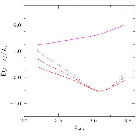
Figure 1: color excess $E(r-z)$ in the observer frame calculated for an absorber at redshift $z_{a}$ with rest-frame extinction $A_{V}=1$ mag. The lines correspond to an SMC-type extinction curve (magenta, solid line; Pei 1992, Gordon et al. 2003) and three MW-type extinction curves (red lines; Cardelli et al. 1998) computed at three values of $R\equiv A_{V}/E(B-V)$ (dots: $R=2.5$; short dashes: $R=3.1$; long dashes: $R=4.0$).

3 The method

3.1 Derivation of the mean color excess

Given two measurements $m_{x}$ and $m_{y}$ of the apparent magnitude of a quasar in two photometric bands $x$ and $y$, we call $C(y-x)=m_{y}-m_{x}$ the quasar color. If dust is present in a foreground absorption system, the observed color will be different from the intrinsic, unreddened color $C_{0}(y-x)$, yielding a color excess $E(y-x)=C(y-x)-C_{0}(y-x)$. This cannot be measured directly since the unreddened color of the individual quasar is unknown. We can however measure the mean color excess of a sample of DLA-quasars in the following way. For each DLA-quasar we build a set of $n_{j}$ unreddened control quasars with same redshift and magnitude. We then estimate the mean color of these unreddened quasars, $\langle C^{u}(y-x)\rangle$, and hence the deviation from the mean color

$$\Delta(y-x)=C(y-x)-\,\langle C^{u}(y-x)\rangle\,.$$ (1)

For a large sample of $n_{i}$ DLA-quasars we measure the mean color excess with the expression

$$\langle E(y-x)\rangle=\langle\Delta(y-x)\rangle\leavevmode\nobreak\ ,$$ (2)

where $\langle\Delta(y-x)\rangle$ is the average of the $n_{i}$ values $\Delta_{i}$. The validity of Eq. (2) is discussed in Appendix A.

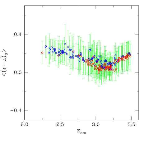
Figure 2: Mean color ${\langle(r-z)_{0}\rangle}$ of the QSOs control samples used to estimate the unreddened colors of the DLA-QSOs. The mean color is plotted versus the QSO redshift, $z_{e}$. Bright ($r<19.1$ mag) and faint ($r\geq 19.1$ mag) QSOs are plotted with blue crosses and red circles, respectively.

3.2 Choice of the color index

Since our ideal goal is to measure the color of the quasar continuum, we excluded photometric bands contaminated by the absorptions in the Ly $\alpha$ forest or the Ly $\alpha$ emission of the quasar. Taking into account the average wavelengths $\overline{\lambda}$ and the FWHMs of the SDSS photometric bands (Fukugita et al. 1996; see also SDSS web page http://www.sdss.org/dr5/instruments/imager) this condition constrains the maximum quasar redshift to $z_{e,\mathrm{max}}=[(\overline{\lambda}-{1\over 2}\,\mathrm{FWHM})/1216]-1=1.67,2.29,3.50,4.52,$ and 5.78 for the $u$, $g$, $r$, $i$, and $z$ bands, respectively. Since the wavelength coverage of SDSS spectra prevents detection of DLA systems at $z_{a}\raisebox{-5.0pt}{$\;\stackrel{{\scriptstyle\textstyle<}}{{\sim}}\;$}2.2$, only the $r$, $i$ and $z$ bands provide quasars with uncontaminated photometry (in the sense specified above) and sufficient redshift coverage for detection of DLA systems. The maximum leverage for reddening detection with these bands is given by the $(r-z)$ color.

3.2.1 The $(r-z)$ color index

In Fig. 1 we plot the color excess $E(r-z)$ in the observer’s frame that we expect to measure for an absorber at redshift $z_{a}$ with rest-frame extinction $A_{V}=1$ magnitude. To estimate $E(r-z)$ we considered different possible types of extinction curves for the dust in the DLA systems, such as the Milky-Way curves by Cardelli et al. (1998), with the characteristic extinction bump at 2175Å, and the SMC curves (Pei 1992, Gordon et al. 2003), characterized by a more regular UV rise. The extinction curves are normalized in the $V$ band, $\xi(\lambda)\equiv A_{\lambda}/A_{V}$, all the quantities in this definition being in the rest frame of the absorber. For an absorber at redshift $z_{a}$ the extinction measured at wavelength $\lambda^{\mathrm{obs}}_{x}$ in the observer’s frame is $A_{\lambda^{\mathrm{obs}}_{x}}=A_{V}\,\xi({\lambda^{\mathrm{obs}}_{x}\over 1+z_{a}})$. The color excess in the observer’s frame per unit extinction in the rest frame is therefore

$${E(\lambda^{\mathrm{obs}}_{y}-\lambda^{\mathrm{obs}}_{x})\over A_{V}}=\delta\xi\,(z_{a};\lambda^{\mathrm{obs}}_{x},\lambda^{\mathrm{obs}}_{y})$$ (3)

where $\delta\xi\,(z_{a};\lambda^{\mathrm{obs}}_{x},\lambda^{\mathrm{obs}}_{y})=\xi({\lambda^{\mathrm{obs}}_{y}\over 1+z_{a}})-\xi({\lambda^{\mathrm{obs}}_{x}\over 1+z_{a}})\leavevmode\nobreak\ .$ From this expression we have computed the curves shown in Fig. 1.

For an SMC-type extinction curve we expect a smooth variation of the predicted color excess in the redshift interval of interest, with a typical value $E(r-z)\simeq 0.15$ mag for absorbers with rest-frame $A_{V}=0.1$ mag. For a MW-type curve we expect a small (or even negative) reddening in the interval of absorption redshift of our sample. The minimum in the MW lines of Fig. 1 corresponds to minimum between the end of the extinction bump at 2175Å and the UV rise. The implications of these different behaviours of the SMC-type and MW-type extinction curves are discussed in Section 5.1.

3.2.2 The $(g-z)$ color index

The measurement of the $(g-z)$ color is challenging because the $g$ band is generally contaminated by the Ly $\alpha$ forest, or even the QSO Lyman break, in the interval of emission redshift considered. However, measuring the reddening in the $(g-z)$ color, in addition of the $(r-z)$ color, offers several advantages. One is the higher leverage for reddening detection: we expect a gain of a factor of $\simeq 2.2$ in the ratio $E(g-z)/E(r-z)$ at the redshift of our sample if the extinction curve is of SMC type. Another advantage is the possibility of probing the wavelength dependence of the reddening, i.e. the extinction curve of the dust, by comparing the $(g-z)$ and $(r-z)$ color excesses. We decided therefore to perform the measurements also in the $(g-z)$ color index taking care of the contaminations present in the $g$ bandpass.

To avoid overlap of the $g$ band with the QSO Lyman break, we restricted the analysis of the $(g-z)$ colors to the QSOs with $z_{e}\leq 3.4$ in our sample. We then took care of the contamination due to Ly $\alpha$ absorptions. The contamination due to the forest is present both in the quasars of the absorption sample and of the control sample. Line-to-line variations of the forest absorption will contribute to the dispersion of the quasar colors, making the measurement of the color excess more difficult. If such variations are randomly distributed, we still can measure the difference between the quasar colors of the absorption and control samples. In doing this, however, we must take into account the fact that the $g$ band of the absorption sample is generally contaminated by the damped Ly $\alpha$ profile, which is absent in the control quasars. To cope with this problem we correct the $g$ magnitude by taking into account the effect of the damped Ly $\alpha$ absorption in the filter bandbass. The magnitudes in the SDSS photometric system are defined as $m=-2.5\,\log\int d(\log\,\nu)\,f_{\nu}\,S_{\nu}+\mathrm{constant}$ (Fukugita et al. 1996), where $f_{\nu}$ is the quasar spectral distribution and $S_{\nu}$ the response function of the filter. We define the correction for the DLA absorption in the $g$ band as

$$\delta m_{g}=-2.5\,\log{\int d(\log\,\nu)\,f^{\circ}_{\nu}\,S^{(g)}_{\nu}\over\int d(\log\,\nu)\,f^{D}_{\nu}\,S^{(g)}_{\nu}}\leavevmode\nobreak\ ,$$ (4)

where $f^{\circ}_{\nu}$ is the quasar spectral distribution without DLA absorption, $f^{D}_{\nu}$ the spectral distribution with DLA absorption, and $S^{(g)}_{\nu}$ the response function of the $g$ filter (Fukugita, 2006, priv. comm.). To estimate $\delta m_{g}$ we model $f^{\circ}_{\nu}$ with a power law with spectral index $\alpha_{\nu}\simeq-0.5$, based on measurements of SDSS spectra of quasars in the redshift interval of interest for the present work (Vanden Berk et al. 2001, Desjacques et al. 2007). For each DLA system of our sample we then compute the theoretical absorption profile of the lines of the Lyman series, $\ell_{\nu}$, with intensity and position of the lines specified by the H i column density and redshift. From this we compute $f^{D}_{\nu}=\ell_{\nu}\times f^{\circ}_{\nu}$ and hence the correction $\delta m_{g}$, which is finally added to the observed magnitude. The theoretical Voigt profiles are computed with the FITLYMAN routines (Fontana & Ballester 1995) included in the ESO MIDAS software package. The typical value of $\delta m_{g}$ is of $\simeq-0.05$ mag, with values as low as $-0.006$ mag and as high as $-0.17$ mag in the most extreme cases.

3.3 Implementation of the method

The “BEST” $ugriz$ imaging data were recovered for all quasars of the absorption and control samples. These photometric data were corrected for the effects of the Galactic extinction according to the prescriptions given by Schneider et al. (2005).

For each quasar of the absorption sample we calculate the colors $(r-z)_{i}$ and $(g-z)_{i}$ and then select a taylored subset of control quasars closest in redshift and magnitude in the following way. We first select the $n_{z_{e}}$ control quasars closest to the redshift $z_{e}$ of the DLA quasar. From this subset we then select the $n_{m}$ control quasars closest to the $z$-band magnitude $m_{z}$ (the least affected by extinction) of the DLA quasar. This last subset is used to estimate the mean unreddened colors ${\langle(r-z)_{0}\rangle}_{i}$ and ${\langle(g-z)_{0}\rangle}_{i}$. The deviations from the mean color are finally calculated as $\Delta_{i}(r-z)=(r-z)_{i}-{\langle(r-z)_{0}\rangle}_{i}$ and $\Delta_{i}(g-z)=(g-z)_{i}-{\langle(g-z)_{0}\rangle}_{i}$.

With this procedure each subset of control quasars has the same size $n_{m}$ for all DLA-QSOs and we have a comparable statistics for all the measurements. The choice of $n_{z_{e}}$ and $n_{m}$ is determined by the requirement that the total intervals in emission redshift, $\delta_{i}(z_{e})$, and $z$ magnitude, $\delta_{i}(m_{z})$, spanned by each subset are sufficiently small to guarantee a good degree of homogeneity of the control samples. In practice, this gives the contraints $n_{z_{e}}\raisebox{-5.0pt}{$\;\stackrel{{\scriptstyle\textstyle<}}{{\sim}}\;$}100$ and $n_{z_{e}}/n_{m}\raisebox{-5.0pt}{$\;\stackrel{{\scriptstyle\textstyle>}}{{\sim}}\;$}4$ in order to have typical (median) values $\delta_{i}(z_{e})\simeq 0.1$ and $\delta_{i}(m_{z})\simeq 0.5$ mag. The redshift interval is similar to the redshift bins commonly adopted in studies of the mean quasar color as a function of $z_{e}$ (e.g. Richards et al. 2001). Changes of the intrinsic slopes of the quasar continua over the above magnitude interval are expected to be modest (Yip et al. 2004).

In Table 1 we report the measurements of $\Delta_{i}(r-z)$ and $\Delta_{i}(g-z)$ for the DLA-QSOs of the absorption sample. In columns 6 and 7 of the table we give the intervals in emission redshift, $\delta_{i}(z_{e})$, and $z$ magnitude, $\delta_{i}(m_{z})$, spanned by each subset of control quasars obtained by adopting $n_{z_{e}}=100$ and $n_{m}=25$. In columns 8 and 9 we list the mean colors $\langle(r-z)_{0}\rangle_{i}$ and $\langle(g-z)_{0}\rangle_{i}$, obtained from the weighted mean of the colors of each control subset. The weights are taken to be proportional to the inverse squares of the errors of individual colors.

The errors of individual colors of DLA quasars and control quasars are obtained by propagation of the photometric errors and of the errors of the Galactic extinction correction. For the latter we adopted an uncertainty of $\pm 50\%$ of the correction itself. The $(g-z)$ data include the correction for damped Ly $\alpha$ absorption in the $g$ band, when approprite. An uncertainty of $\pm 50\%$ of this correction is propagated in the error budget.

The errors of the mean colors ${\langle(r-z)_{0}\rangle}_{i}$ and $\langle(g-z)_{0}\rangle_{i}$ quoted in Table 1 are the standard deviation of the colors of each subset. These errors dominate the budget of the errors of the color deviations $\Delta_{i}(r-z)$ and $\Delta_{i}(g-z)$.

In Fig. 2 we plot the mean colors ${\langle(r-z)_{0}\rangle}_{i}$ of the subsets of unreddened quasars versus $z_{e}$. Each data point corresponds to the subset of an individual DLA-quasar of Table 1. We use different symbols for quasars brighter and fainter than the median magnitude of the absorption sample, $m_{r}=19.1$. In addition to a trend with $z_{e}$, known from previous studies, the figure shows a dependence on the quasar magnitude. For instance, at $z_{e}\approx 3$, where many quasars both fainter and brighter than $m_{r}=19.1$ are present, the fainter quasars (red circles) lie systematically below the brighter ones (blue crosses). This result justifies our choice of grouping the control quasars not only in redshift, but also in magnitude.

Table 3: Mean reddening in the observer’s frame, $\langle E\rangle$, and mean extinction in the rest frame, $\langle A_{V}\rangle$, for different colors and DLA/QSO samples.

color			$(r-z)$				$(g-z)$
Redshift interval			$2.25\leq z_{e}\leq 3.5$				$2.25\leq z_{e}\leq 3.4$
Absorption	$n$	${\langle E(r-z)\rangle}$	$\langle A_{V}\rangle$	$\langle A_{V}/N({H\textsc{i}})\rangle$	$n$	${\langle E(g-z)\rangle}$	$\langle A_{V}\rangle$	$\langle A_{V}/N({H\textsc{i}})\rangle$
sample		[10-3 mag]	[10-3 mag]	[10-23 mag cm2]		[10-3 mag]	[10-3 mag]	[10-23 mag cm2]
1a	248	27 $\pm$ 8.8	19 $\pm$ 5.9	4.1	232	54 $\pm$ 12	17 $\pm$ 3.8	3.2
2b	247	24 $\pm$ 8.3	17 $\pm$ 5.6	3.5	231	51 $\pm$ 12	16 $\pm$ 3.7	2.8
3c	246	22 $\pm$ 8.0	16 $\pm$ 5.4	3.0	229	48 $\pm$ 11	15 $\pm$ 3.5	2.4
Bootstrapd	248	27 $\pm$ 9.2			232	54 $\pm$ 14

^a Complete absorption sample of Table 1.

^b Cases with $\Delta_{i}>\langle\Delta\rangle+5\times\sigma$ are excluded from the complete sample ($\sigma=\sigma_{m}\times\sqrt{n}$). ^c Cases with $\Delta_{i}>\langle\Delta\rangle+3\times\sigma$ are excluded from the complete sample. ^d Mean and standard deviation of the mean color excess of 10,000 bootstrap samples obtained from the absorption sample 1.

4 The mean color excess

In Table 3 we give the weighted means ${\langle E(r-z)\rangle}$ and ${\langle E(g-z)\rangle}$ estimated with the expression ${\langle E\rangle}=\langle\Delta\rangle=\sum_{i}w_{i}\Delta_{i}$, where $w_{i}=\sigma_{i}^{-2}/\sum_{i}\sigma_{i}^{-2}$, and $\sigma_{i}$ are the errors of individual measurements. The use of the weighted mean allows us to minimize the contribution of the QSOs with largest uncertainty of their intrinsic colors, the dominant source of the error budget.

For the error of the mean we adopted the unbiased estimate

$$\sigma_{m}=\sqrt{\sum_{i}w_{i}\,(\,\Delta_{i}-{\langle\Delta\rangle}\,)^{2}\over(n-1)}$$ (5)

(Linnik 1961) with the normalized weights $w_{i}$ given above. This expression is valid if the measurements of $\Delta_{i}$ are uncorrelated. We performed two tests to make sure that correlated errors are unimportant and therefore the adopted statistical error $\sigma_{m}$ is reliable. First we computed the covariance matrix and compared the strength of off-diagonal terms with that of diagonal terms. The covariance matrices of the $\Delta_{i}(r-z)$ and $\Delta_{i}(g-z)$ data samples were computed using a bootstrap method over 60 random realizations of each sample. We found that the normalized covariance matrices are fairly close to be diagonal, with off-diagonal terms tipically around a few percent, and always below 25%. The low values of the off-diagonal terms indicate that there is little correlation between the measurements. Then we studied the behaviour of $\sigma_{m}$ as a function of the sample size. This can be done with a random grouping technique described by Hampel et al. (1986; Chap.8). From this test we find that the adopted error follows the theoretical $n^{-0.5}$ decrease, as expected for uncorrelated measurements. The adopted error of the mean is therefore a good estimate of the statistical error of $\langle E\rangle$.

4.1 Confidence level of detection

From the results shown in Table 3 one can see that the mean $(r-z)$ reddening is detected at $\simeq 3\,\sigma_{m}$ confidence level (statistical error) in the complete sample of 248 DLA/QSO pairs for which the $r$ band is uncontaminated by Ly $\alpha$ forest ($z_{e}\leq 3.5$). The mean $(g-z)$ reddening is detected at $\simeq 4.5\,\sigma_{m}$ confidence level in the sample of 232 DLA/QSO pairs with $g$ magnitude uncontaminated by the QSO Lyman break ($z_{e}\leq 3.4$) and corrected for DLA flux suppression (Section 3.2.2).

To estimate the confidence level of the detection other than in terms of $\sigma_{m}$ we applied the method of bootstrap resampling (Efron 1979). A bootstrap sample is obtained by extracting $n$ data at random with repetition from the original sample of $n$ measurements. This type of extraction is, in practice, an extraction with replacement because part of the original measurements is replaced by repeated data. By iterating this extraction process many times it is possible to build a large number $N_{B}$ of bootstrap samples from the original set of $n$ data. For each of the $N_{B}$ samples one can compute a statistical estimator of interest (e.g. the weighted mean) and study the distribution of such estimator, without making any assumption on the parent distribution. We applied this method to the original sample of $n$ measurements $\Delta_{i}$, from which we built up $N_{B}=10,000$ bootstrap samples. The weighted mean $\langle\Delta\rangle$ was recomputed in each case. We analyzed the resulting distribution of $\langle\Delta\rangle$ values (Fig. 3) to estimate the fraction of cases in which the mean value is positive. We find $\langle\Delta(r-z)\rangle>0$ in $\simeq 99.90\%$ of the $\Delta_{i}(r-z)$ bootstrap samples and $\langle\Delta(g-z)\rangle>0$ in $\simeq 99.99\%$ of the $\Delta_{i}(g-z)$ bootstrap samples. These percent figures indicate the probability that a positive color excess has been detected.

4.2 Analysis of “twin control samples”

A reason of concern in the present analysis is the possibility that the mean color excess that we detect is due to sources of reddening other than the DLA systems (e.g. dust in the quasar environment or in unidentified absorbers). If present, these reddening contribution would also affect the quasars of the control sample. To understand if these effects may accidentally yield a mean color excess comparable to that measured in the DLA sample, we applied our procedure to a large number of “twin control samples” with same size, redshift distribution and magnitude distribution as the DLA sample. We then analyzed the values of $\langle\Delta\rangle$ obtained from these twin control samples in a search for cases with a value equal to those reported in Table 3. In practice, each twin control sample was created by extracting at random, for each DLA-QSO of Table 1, a control QSO at the same redshift and magnitude. The control QSOs extracted in this way were treated as DLA-QSOs and temporarily excluded from the estimate of the mean unreddened colors $\langle C^{u}\rangle$ (Section 3.1). As a consequence, the estimates of $\langle C^{u}\rangle$ were different for each realization of the twin control sample. We built up 10,000 twin control samples and computed the weighted mean $\langle\Delta\rangle$ for each of them. The resulting frequency distribution of $\langle\Delta\rangle$ values is shown in Fig. 4 for both color indices of interest. For comparison we show the mean color excess of the absorption sample (dotted lines). The probability for a twin control sample to attain a value $\langle\Delta\rangle$ as high as the mean color excess of the absorption sample is $<0.01\%$ in $(g-z)$ and $\simeq 0.4\%$ in $(r-z)$. We conclude that the mean color excess detected in the absorption sample cannot be ascribed to dust in the quasar environment or in unidentified low-redshift absorbers. The same low probability applies to any sort of systematic effect that might accidentally conspire to yield a mean color excess as a consequence of the application of our procedure to a quasar sample with same size, redshift distribution and magnitude distribution as the DLA sample.

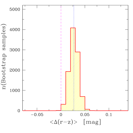
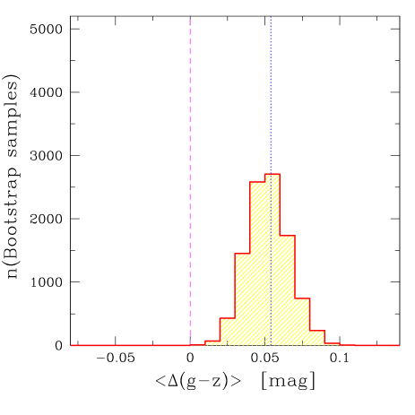
Figure 3: Frequency distribution of the mean color excess $\langle\Delta(r-z)\rangle$ and $\langle\Delta(g-z)\rangle$ measured in 10,000 bootstrap samples obtained from the list of $\Delta$ values of Table 1. Dotted line: mean color excess of the original sample. See Section 4.1.

4.3 Rejection of the most reddened quasars

For a correct interpretation of the present results it is important to understand whether the mean reddening that we detect is a signature of the bulk of the DLA population or is just due to the presence of a few reddened quasars. To clarify this point we rejected the most reddened DLA-QSOs from the original sample of Table 1 and repeated the computation of the mean reddening. In practice, we discarded the cases with individual color deviation $\Delta_{i}$ larger than the mean color deviation $\langle\Delta\rangle$ at $5\,\sigma$ level (“absorption sample 2”) and at $3\,\sigma$ level (“absorption sample 3”). In the second and third row of Table 3 we show the mean color excess recomputed after rejecting the most reddened cases in this way. One can see that the mean color excess is still detected at $\simeq$ 2.8 $\sigma_{m}$ level in $(r-z)$ and at 3.5 $\sigma_{m}$ level in $(g-z)$ for the absorption sample 3. The detection is firmer for the absorption sample 2.

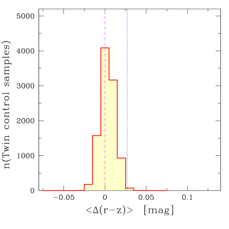
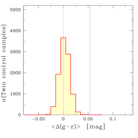
Figure 4: Frequency distribution of the mean deviations $\langle\Delta(r-z)\rangle$ and $\langle\Delta(g-z)\rangle$ measured in 10,000 control samples with identical size, redshift distribution and magnitude distribution of the absorption sample. Dotted line: mean color excess of the absorption sample. See Section 4.1.

4.4 Size of the subsets of control quasars

As an final test we checked the stability of the results for the adoption of different values of $n_{z_{e}}$ and $n_{m}$ (Section 3.3). We tested this effect by varying these parameters around their optimal values $n_{z_{e}}\simeq 100$ and $n_{z_{e}}/n_{m}\simeq 4$. The resulting changes of the mean reddening are significantly smaller than the statistical error discussed above.

5 Discussion

The analysis presented in the previous section indicates that high-redshift quasars with intervening DLA systems at $2.2\leq z_{a}\leq 3.5$ have redder colors than quasars at the same redshift without foreground absorption systems.

The most natural process to explain the origin of this reddening is dust extinction, with its characteristic rise at shorter wavelengths. If this is the case, we expect the measured reddening to show similarities with that predicted for typical interstellar dust extinction curves. We also expect the most reddened quasars to be dimmed by dust extinction and therefore to be statistically fainter than unreddened quasars. In Sections 5.1 and 5.2 below we present observational evidence consistent with these expectations.

The location of the dust is of special interest in the present work. Reddening sources in the quasar environment cannot explain the difference in color between the quasars of the absorption and control samples since this type of reddening would affect in the same way, on the average, the quasars of both samples. Dust embedded in the DLA systems is the most natural hypothesis to explain the measured color excess. This hypothesis bears some predictions that can be tested empirically.

One is that the reddening should increase with the column density of the metals embedded in the DLA systems. Another is that the dust-to-gas ratio should approximately scale with the level of metallicity of DLA systems. In Sections 5.3 and 5.4 below we present observational evidence consistent with these expectations. In Sections 5.5 and 5.6 we discuss the reddening versus H i column density and versus absorption redshift.

5.1 Dust extinction curve

One of the properties used to characterize the interstellar dust is its extinction curve, $\xi(\lambda)\equiv A_{\lambda}/A_{V}$. In spite of strong spatial variability, interstellar extinction curves can be classified in two types: Milky-Way type curves, with the characteristic extinction bump at 2175 Å (e.g. Cardelli et al. 1998), and SMC-type curves, characterized by a more regular UV rise (e.g. Pei 1992, Gordon et al. 2003). The different slopes of these curves can be used to distinguish between them.

If the reddening originates in the DLA systems, we can measure the slope of the DLA dust extinction curve by comparing the mean reddening in the $(g-z)$ and $(r-z)$ colors. We use the restricted sample of 232 DLA-QSOs with $z_{\mathrm{em}}<3.4$, for which both $(g-z)$ and $(r-z)$ can be derived. For this sub-sample we measure $\langle E(r-z)\rangle=25(\pm 9.0)$ 10^-3 mag and we obtain $\langle E(g-z)\rangle/\langle E(r-z)\rangle=$ 2.2 $\pm$ 0.9. This measurement is in good agreement with the ratio predicted for absorbers with SMC-type extinction curve at $2.2\leq z_{a}\leq 3.5$, $\langle E(g-z)/E(r-z)\rangle^{\mathrm{SMC}}_{\mathrm{pred}}\simeq 2.2$.

The fact that we detect reddening in the $(r-z)$ color argues againts a MW-type extinction curve. In fact, this type of curve is expected to give a negligible or even negative reddening in the interval of absorption redshift spanned by of our sample (Fig. 1). This is due to the fact that in this interval the $(r-z)$ color probes a part of the MW extinction curve with negative slope, namely the end of the 2175 Å extinction bump. The fact that we detect reddening in the $(r-z)$ color indicates that extinction curve of MW type must be uncommon in the sample.

If DLAs with MW-type curves exist, a broad absorption centered at $(1+z_{a})\times 2175\,\AA$ should affect the quasar continuum. We searched for this feature in all the spectra of the absorption sample, and in particular of the quasars with anomalous colors, but without success (see e.g. Fig. 8).

The above results are in line with the general finding that MW-type extinction curves are rare among quasar absorbers (Junkkarinen et al. 2004, Wang et al. 2004), while SMC-type are common (Wild & Hewett 2005, York et al. 2006). By adopting an SMC extinction curve, our results imply a rest-frame extinction $\langle A_{V}\rangle\simeq 0.015/0.019$ mag (Table 3), corresponding to $\langle E(B-V)\rangle\simeq 0.005/0.007$ mag.

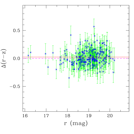
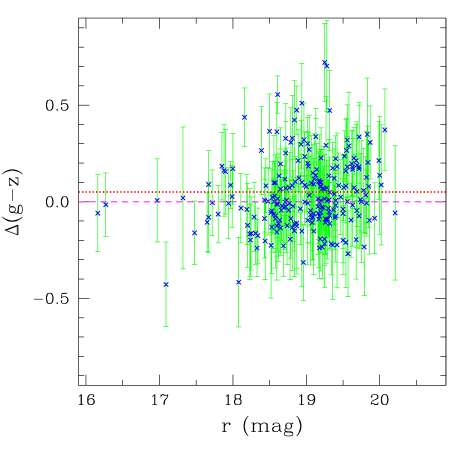
Figure 5: Deviation from the mean color, $\Delta(r-z)$ and $\Delta(g-z)$, versus $r$ magnitude for sample 2 of Table 3. Dotted lines: mean color excess of the same sample.

5.2 Reddening versus quasar magnitude

As we mentioned above, we expect the most reddened quasars to be statistically fainter than unreddened quasars if the reddening originates in dust. In Fig. 5 we plot $\Delta(r-z)$ and $\Delta(g-z)$ versus the $r$ magnitude. The largests values of color excess lie at faint magnitudes ($r\raisebox{-5.0pt}{$\;\stackrel{{\scriptstyle\textstyle>}}{{\sim}}\;$}18$ mag), in broad agreement with this expectation. To quantify the effect we compared the mean magnitude of the 30 DLA-QSOS with highest $\Delta(r-z)$ with the mean magnitude of the remaining DLA-QSOs with lower $\Delta(r-z)$. The most reddened cases are slightly fainter on the average, $\langle r\rangle=19.24\pm 0.08$, than the remaining cases, $\langle r\rangle=18.98\pm 0.04$. A similar computation for the $(g-z)$ color yields $\langle r\rangle=19.11\pm 0.09$ for the 30 most reddened cases and $\langle r\rangle=18.96\pm 0.05$ for the remaining cases. The effect is modest, but is in line with the prediction that quasars with higher reddening should be statistically fainter.

Table 4: Mean reddening of sub-samples with different strengths of the Si ii 1526 line detected at the redshift of the DLA system.

		$W_{{Si\textsc{ii}}}$	$<1$ Å	$W_{{Si\textsc{ii}}}$	$\geq 1$ Å
color	Sample	$n$	$\langle E\rangle$	$n$	$\langle E\rangle$
			[10-3 mag]		[10-3 mag]
$(r-z)$	1	$151$	$26\pm 12$	$29$	$41\pm 25$
	2	$150$	$21\pm 11$	$29$	$41\pm 25$
	3	$149$	$17\pm 10$	$29$	$41\pm 25$
$(g-z)$	1	$142$	$51\pm 14$	$29$	$114\pm 40$
	2	$141$	$46\pm 13$	$29$	$114\pm 40$
	3	$140$	$42\pm 13$	$29$	$114\pm 40$

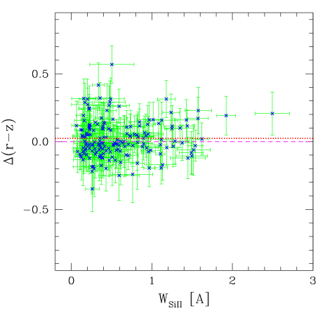
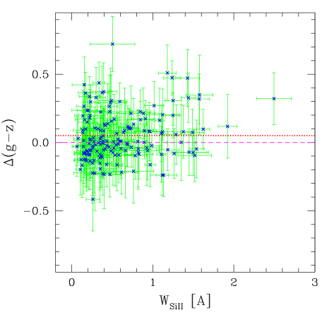
Figure 6: Deviations from the mean color, $\Delta(r-z)$ and $\Delta(g-z)$, versus rest-frame equivalent width of Si ii line 1526Å, when detected, for sample 2 of Table 3. Dotted lines: mean color excess of the same sample.

5.3 Reddening versus metal column density

If the reddening originates in dust embedded in the DLA system we expect a trend between the color excess and the total column density of metals in the absorber. The limited spectral resolution of SDSS spectra prevents the accurate measurement of metal column densities, but is sufficient to measure the equivalent width of strong metal lines. To search for a possible trend between color excess and metals we performed a study of the Si ii line at 1526 Å, which is sufficiently strong to be detected in SDSS spectra and lies redwards of the Ly $\alpha$ forest in most of the redshift range of interest. Since the 1526 Å line is saturated, its rest-frame equivalent width, $W_{Si\textsc{ii}}$, is not a good tracer of the metal column density. Nevertheless, an empirical correlation between $W_{Si\textsc{ii}}$ and metallicity has been recently found for DLA-QSOs, in the form [M/H] $\simeq-0.92+1.41\,\log W_{Si\textsc{ii}}$ (Prochaska et al. 2007). This correlation is probably the consequence of the mass-metallicity and mass-kinematics relations in galaxies. Galaxies with higher masses (and metallicities) have larger kinematical motions, which result in larger spread (and equivalent width) of saturated metal lines such as the Si ii line at 1526 Å.

To estimate $W_{Si\textsc{ii}}$ we used an automated algorithm which fits a Gaussian profile to the strongest absorption feature (if any) at the predicted wavelength, $\lambda_{{Si\textsc{ii}}}=(1+z_{a})\,1526.707$ Å, provided this line occurs redwards of the Ly $\alpha$ forest. Each fit was visually inspected and the line-strength of Si ii 1526 was compared against other metal-lines observed redwards of the Ly$\alpha$ forest. In a few cases, we rejected lines because of obvious blends with coincident absorption lines from systems at unrelated redshifts. As a result of this analysis, we measured an equivalent width in 180 DLA-QSOs of our sample. In Fig. 6 we plot the deviations from the mean colors $\Delta(r-z)$ and $\Delta(g-z)$ versus the rest-frame equivalent width $W_{Si\textsc{ii}}$ measured by the automated algorithm. No clear trend is present, possibly because most of the data are clumped at low values of equivalent width, where we expect a modest reddening. The interval $W_{Si\textsc{ii}}>1\,\AA$, where the reddening is expected to be stronger, is much less populated, but its size is sufficiently large to compute the mean value. We therefore splitted the data in two subsets of “weak” and “strong” Si ii absorbers by using $W_{Si\textsc{ii}}=1\,\AA$ as a threshold value. The mean values of reddening derived for these subsets are shown in Table 4 for the three absorption samples defined in Table 3. One can see that the mean reddening tends to be higher in strong Si ii absorbers than in weak Si ii absorbers, as expected if the dust is embedded in DLA systems. The difference in mean reddening between the two sub-samples is marginal in the $(r-z)$ color, but more evident in the $(g-z)$ color.

To investigate the physical relation between dust and metals we converted the color deviations $\Delta$ into a mean extinction and the Si ii equivalent widths into a metallicity. The rest-frame extinction, $A_{V}$, is expected to scale with the metal column density $\mathrm{(M/H)}\times N({H\textsc{i}})$, where (M/H) is the total abundance by number (gas plus dust) of the reference element M (e.g. Vladilo et al. 2006).

To derive the extinction we used the expression $A_{V}=E(\lambda^{\mathrm{obs}}_{y}-\lambda^{\mathrm{obs}}_{x})\,/\,\delta\xi\,(z_{a};\lambda^{\mathrm{obs}}_{x},\lambda^{\mathrm{obs}}_{y}),$ obtained from Eq. (3). The true color excess $E_{i}$ of the individual quasar is unknown, but we can take $E_{i}\simeq\Delta_{i}$ since we average the above expression for a large sample to obtain $\langle A_{V}\rangle$ (see Section 3.1). An SMC extinction curve $\xi(\lambda)$ was adopted in this conversion.

To derive the metal column density we used the empirical relation [M/H] $\simeq-0.92+1.41\,\log W_{Si\textsc{ii}}$ (Prochaska et al. 2007) and then averaged the individual values of metal column density $10^{\mathrm{[M/H]}+\log N({H\textsc{i}})}$.

In Fig. 7 we plot the results of these computations obtained for the subsets of weak and strong Si ii absorbers of Table 4 (sample 2). The data are consistent with the existence of the trend between metal column density and extinction expected if the reddening and metals originate in the same medium. Again, the evidence for this trend is very weak in $(r-z)$ and firmer in $(g-z)$. Given the uncertainties in the above conversions and the limited statistics it is not possible to reach firmer conclusions.

The quasars of the absorption sample with high color deviations and strong Si II absorptions are excellent candidates for detailed follow up studies of dusty DLA systems based on high resolution spectroscopy. In Fig. 8 we show, as an example, the spectra of the DLA-quasars with $\Delta(g-z)>0.4$ and $W_{Si\textsc{ii}}>1\,\AA$. The typical metallicity of these systems is a factor 3 larger than the average metallicity of the absorption sample.

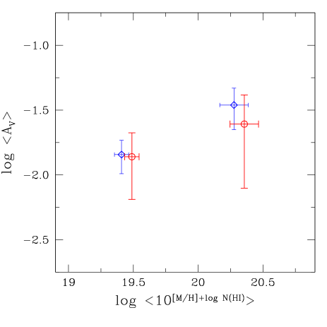
Figure 7: Mean values of rest-frame extinction and metal column density of the two subsets of DLA-QSOs with different strengths of the Si ii line 1526 Å shown in Table 4 (absorption sample 2). The extinction values derived from the $(g-z)$ and $(r-z)$ color deviations are plotted with diamonds and circles, respectively. The mean values of metal column density of the two subsets are the same and have been slightly shifted along the horizontal direction for clarity. See Section 5.3.

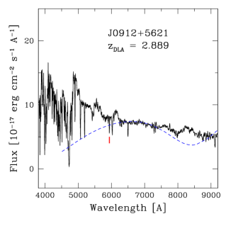
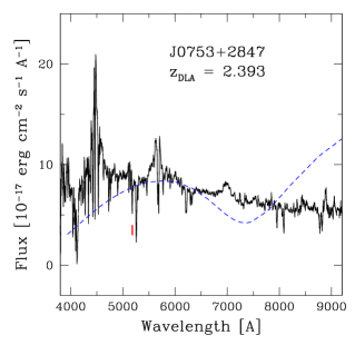
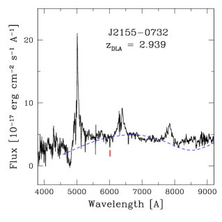
Figure 8: Quasars of the absorption sample with color deviations $\Delta(g-z)>0.4$ mag and strong Si ii absorptions at $z_{\mathrm{SiII}}=z_{\mathrm{DLA}}$. Dashed line: profile of the 2175 Å extinction bump plotted in a scale $10^{-\xi[\lambda/(1+z_{\mathrm{DLA}})]}$ (see Vladilo et al. 2006).

5.4 Dust-to-gas ratio

By adopting an extinction curve $\xi(\lambda)$ of SMC-type we can convert the reddening measured in the observer’s frame into an extinction in the rest frame. From this in turn we can measure, for the first time in studies of DLA systems, the dust-to-gas ratio in the same units used in local interstellar studies, namely the ratio $A_{V}/N({H\textsc{i}})$ between the extinction in the $V$ band and the H i column density. From Eq.(3) the individual dust-to-gas ratio is given by

$${A_{V}\over N({H\textsc{i}})}={E(\lambda^{\mathrm{obs}}_{y}-\lambda^{\mathrm{obs}}_{x})\,/\,\delta\xi\,(z_{a};\lambda^{\mathrm{obs}}_{x},\lambda^{\mathrm{obs}}_{y})\over N({H\textsc{i}})}\leavevmode\nobreak\ .$$ (6)

Since we average this quantity for all the systems of our sample we take $E_{i}\simeq\Delta_{i}$ (see Section 3.1). The mean values obtained from this computation are shown in Table 3. We obtain $\langle A_{V}/N({H\textsc{i}})\rangle\simeq$ 3 to 4 $\times 10^{-23}$ mag cm², from the measurements in the $(r-z)$ or $(g-z)$ colors, respectively. By excluding the most reddened cases we obtain $\langle A_{V}/N({H\textsc{i}})\rangle\simeq$ 2.5 to 3.5 $10^{-23}$ mag cm². For comparison, the typical dust-to-gas ratio of the Milky Way is $A_{V}/N({H\textsc{i}})\approx 5.3\times 10^{-22}$ mag cm² (Bohlin et al. 1978). These results indicate that the dust-to-gas ratio of DLA systems is deficient by $\approx-1.25$ dex relative to that of the Milky Way. This deficiency is consistent with the lower level of metallicity of the DLA systems of our sample. This metallicity can be estimated from the relation between [M/H] and $W_{Si\textsc{ii}}$ (Prochaska et al. 2007). For the systems with measurements of $W_{Si\textsc{ii}}$ we obtain a mean value $\langle\mathrm{[M/H]}\rangle\simeq-1.2$ dex (Table 5). We conclude that the dust-to-gas ratio scales with the metallicity, as expected for dust embedded in the DLA galaxies.

Table 5: Mean metallicity and extinction per unit metal column density for the DLA-QSOs with Si ii measurements.

color			$(r-z)$				$(g-z)$
Absorption	$n$	${\langle\mathrm{[M/H]}\rangle}^{b}$	${\langle\mathrm{[M/H]}\rangle}_{w}^{c}$	$\langle s_{V}^{\mathrm{Fe}}\rangle^{d}$	$n$	${\langle\mathrm{[M/H]}\rangle}^{b}$	${\langle\mathrm{[M/H]}\rangle}_{w}^{c}$	$\langle s_{V}^{\mathrm{Fe}}\rangle^{d}$
samplea				[10-17 mag cm2]				[10-17 mag cm2]
1	180	$-1.19\pm 0.03$	$-1.07$	14 $\pm$ 8	171	$-1.18\pm 0.03$	$-1.07$	7.5 $\pm$ 4.3
2	179	$-1.18\pm 0.03$	$-1.07$	12 $\pm$ 8	170	$-1.18\pm 0.03$	$-1.06$	5.8 $\pm$ 4.0
3	178	$-1.18\pm 0.03$	$-1.07$	11 $\pm$ 8	169	$-1.17\pm 0.03$	$-1.06$	5.4 $\pm$ 4.0

^a Absorption samples are defined in Table 3. Only cases with Si ii line detected at more than 1 $\sigma$ level are considered in this table.

^b Mean metallicity $\langle\mathrm{[M/H]}\rangle\equiv\log\,\langle 10^{\mathrm{[M/H]}}\rangle$. The quoted error is the standard error of the mean. ^c Mean H i column-density weighted metallicity of Eq. (9). ^d Mean extinction per unit dust column density of iron (Section 5.5). The quoted error is the standard error of the mean.

5.5 Dust-to-metal ratio

The present measurements of reddening and metallicity can be combined to estimate the mean extinction per unit metal column density in the DLA systems of our sample. We start from the relation

$$A_{V}=\langle s_{V}^{\mathrm{Fe}}\rangle\times f_{\mathrm{Fe}}\times\mathrm{(Fe/H)}\times N({H\textsc{i}})\leavevmode\nobreak\ ,$$ (7)

where $\langle s_{V}^{\mathrm{Fe}}\rangle$ is the mean extinction per unit dust column density of iron and $f_{\mathrm{Fe}}$ is the fraction of iron in dust form (Vladilo et al. 2006). Previous measurements of $\langle s_{V}^{\mathrm{Fe}}\rangle$ have yielded a typical value $\langle s_{V}^{\mathrm{Fe}}\rangle\approx 3\times 10^{-17}$ mag cm², roughly constant within a factor of two, in different types of H i interstellar regions, including metal absorption systems and a few DLA systems at $z_{a}\raisebox{-5.0pt}{$\;\stackrel{{\scriptstyle\textstyle<}}{{\sim}}\;$}2$. The present data set allows us to investigate whether or not this parameter has a similar value also in the general population of DLA systems at $z_{a}\raisebox{-5.0pt}{$\;\stackrel{{\scriptstyle\textstyle>}}{{\sim}}\;$}2$.

By combining the Eqs. (7) and (3) we obtain

$$\langle s_{V}^{\mathrm{Fe}}\rangle={E(\lambda^{\mathrm{obs}}_{y}-\lambda^{\mathrm{obs}}_{x})\,/\,\delta\xi\,(z_{a};\lambda^{\mathrm{obs}}_{x},\lambda^{\mathrm{obs}}_{y})\over f_{\mathrm{Fe}}\times(\mathrm{Fe/H})\times N({H\textsc{i}})}\leavevmode\nobreak\ .$$ (8)

As in the previous section, we take $E_{i}\simeq\Delta_{i}$ because we average this expression for all the systems of our sample. We adopt an SMC extinction curve, assume (Fe/H) $=$ (M/H) and take $f_{\mathrm{Fe}}\simeq 0.65$, a value appropriate for DLA systems at the redshift of our sample (Vladilo 2004). The resulting values of $\langle s_{V}^{\mathrm{Fe}}\rangle$, shown in Table 5, are broadly consistent with the value $\langle s_{V}^{\mathrm{Fe}}\rangle\approx 3\times 10^{-17}$ mag cm² inferred from previous investigations at lower redshift. This is true, in particular, for our best estimate obtained from the $(g-z)$ color deviations. Considering the uncertainties in the values of $f_{\mathrm{Fe}}$ and (Fe/H), this broad agreement is rather remarkable and suggests that the extinction properties of the dust are similar to those of low-redshift dust. A firmer conclusion must await more accurate determinations of the metallicities and depletions of the present sample.

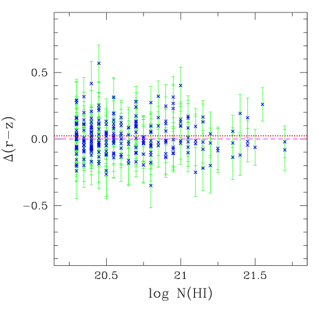
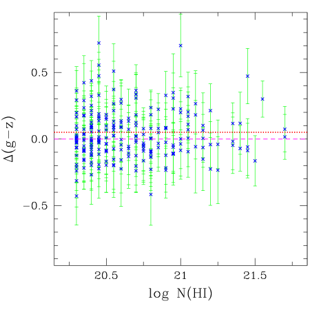
Figure 9: Deviations from the mean color, $\Delta(r-z)$ and $\Delta(g-z)$, versus H i column density for sample 2 of Table 3. Dotted lines: mean color excess of the same sample.

5.6 Reddening and H i column density

In Fig. 9 we plot the color deviations $\Delta(r-z)$ and $\Delta(g-z)$ versus H i column density. A linear correlation analysis of $\Delta(r-z)$ and $\Delta(g-z)$ versus $\log N$(H i) for the complete absorption sample yields correlation coefficients $r=-0.01$ and $r=+0.01$, respectively. The comparison of sub-samples with low and high values of $N$(H i) does not indicate the existence of a trend with reddening. Most DLA-QSOs are concentrated at low H i column densities as a consequence of the well-known decrease of the number of DLA systems with increasing $N({H\textsc{i}})$ (Wolfe et al. 2005; Prochaska et al. 2005). Some of the most reddened quasars are concentrated at low H i column densities, at odd with the expectation that large reddening is associated with large column density of neutral gas. The paucity of highly reddened cases at $N({H\textsc{i}})>10^{21}$ atoms cm^-2 could be the consequence of low-number statistics: systems with high H i column density are rare and the present statistics might be insufficient to detect cases of high reddening. It is worth noticing that lines of sight of high metallicity are generally not observed in DLA systems with $N({H\textsc{i}})>10^{21}$ atoms cm^-2 (Boissé et al. 1998). If this is the case also for the present sample, this fact could conspire to make rare the systems of high reddening at $N({H\textsc{i}})>10^{21}$ atoms cm^-2.

5.7 The H i column-density weighted metallicity

The metal abundances of DLA systems are often used to estimate the mean cosmic metallicity of the neutral gas at high redshift. In this type of estimate the metallicity of each system must be weighted by its H i column density to estimate a mean cosmic value

$$\langle\mathrm{[M/H]}\rangle_{w}={\sum_{i}\,(\mathrm{M/H})_{i}\times N_{i}({H\textsc{i}})\over\sum_{i}N_{i}({H\textsc{i}})}$$ (9)

(Lanzetta et al. 1995). We estimated the above expression by using the indirect measurement of metallicity obtained from the equivalent width of the Si ii line. The results are shown in Table 5. We obtain $\langle\mathrm{[M/H]}\rangle_{w}\simeq-1.1$ dex. This value is somewhat higher than the mean H i-weighted metallicity of DLA systems measured in high-resolution surveys at redshift $z_{a}\approx 3$, which is $\simeq-1.5$ dex (Prochaska et al. 2001; Kulkarni et al. 2005). The present survey of low-resolution SDSS quasar spectra is characterized by a higher magnitude limit since it includes quasars as faint as $m_{r}=20.2$. The higher value of metallicity of the present SDSS sample suggests that the mean metallicity of DLAs may increase with the limiting magnitude of the survey. An effect of this type is predicted as a consequence of the dust extinction bias (Ellison et al. 2001, Vladilo & Pèroux 2005), but the empirical evidence for its existence is still lacking (Akerman et al. 2005). An accurate determination of the metallicities of the present absorption sample will offer us a way to test the dependence of the mean metallicity on the limiting magnitude of DLA-QSO surveys.

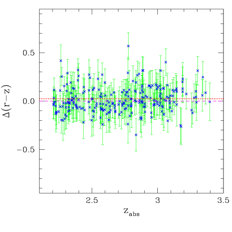
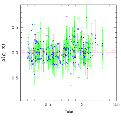
Figure 10: Deviations from the mean color, $\Delta(r-z)$ and $\Delta(g-z)$, versus absorption redshift for sample 2 of Table 3. Dotted lines: mean color excess of the same sample.

5.8 Reddening versus DLA redshift

In Fig. 10 we plot the color deviations $\Delta(r-z)$ and $\Delta(g-z)$ versus absorption redshift $z_{a}$. The data are spread more or less uniformly in the interval of absorption redshift considered. A linear correlation analysis of $\Delta(r-z)$ and $\Delta(g-z)$ versus $z_{a}$ for the complete absorption sample yields correlation coefficients $r=+0.13$ and $r=+0.06$, respectively. The lack of a trend with redshift implies that the color excess that we derive is sufficiently representative of the mean reddening of DLA systems over the full interval $2.2\raisebox{-5.0pt}{$\;\stackrel{{\scriptstyle\textstyle<}}{{\sim}}\;$}z_{a}\raisebox{-5.0pt}{$\;\stackrel{{\scriptstyle\textstyle<}}{{\sim}}\;$}3.5$ covered by our sample. The lack of redshift evolution is, to some extent, surprising. Two types of evolutionary effects are expected to occur if the reddening originates in DLA dust. On the one hand, a rise of the reddening with increasing $z_{a}$ is expected due the UV rise of the extinction curve. For an SMC extinction curve this effect is roughly a factor of 2 in $E(r-z)$ in the redshift range of interest, as shown in Fig. 1. On the other hand, a decrease of the reddening with increasing $z_{a}$ is expected as a consequence of cosmic chemical evolution if the dust scales with the metals. Also this effect is expected to be approximately a factor of 2 in the redshift interval of interest, where the mean metallicity decreases by $\simeq 0.3$ dex per unit redshift interval (Prochaska et al. 2000). The lack of a trend could be the consequence of the opposite behaviour of two evolutionary effects, which tend to cancel each other.

5.9 Comparison with previous work

To perform a homogeneous comparison with the work of Murphy & Liske (2004; ML04) we applied our procedure to their original list of quasars extracted from the second data release (DR2). The list includes 70 DLA-quasars and 1396 non-DLA quasars in spectra with SNR $\geq 3$ as defined in ML04. To apply our procedure we selected the 56 DLA-quasars and 1074 non-DLA quasars with $z_{e}\leq 3.5$. The non-DLA quasars were used to build the control pool. From the application of our method to these lists we obtain the weighted mean values $\langle E(r-z)\rangle=3\,(\pm 22)\times 10^{-3}$ mag and, for the subset of 52 quasars with $z_{e}\leq 3.4$, ${\langle E(g-z)\rangle}=39\,(\pm 36)\times 10^{-3}$ mag. The lack of detection of the reddening is due to the small size of the sample. By converting these results to rest-frame color excess with an SMC extinction curve we obtain a $3\sigma$ upper limit $E(B-V)<0.02$ mag from both color indices. This limit is equal to that obtained by ML04 from their analysis of the spectral index distribution of the quasar spectra. The photometric method presented here and the spectral index method adopted by ML04 yield therefore consistent results.

6 Summary and conclusions

We have used the spectroscopic and photometric database of the 5th data release of the SDSS to measure the reddening of quasars with intervening Damped Ly $\alpha$ systems at high redshift ($z_{\mathrm{DLA}}>2.2$). The spectroscopic database was used to distinguish quasars with and without intervening absorption systems. Only good quality spectra, with typical signal-to-noise ratio SNR $\raisebox{-5.0pt}{$\;\stackrel{{\scriptstyle\textstyle>}}{{\sim}}\;$}4$ in the spectral regions of interest, were considered in the analysis. We built up an “absorption sample” of 248 quasars with a single DLA system in the redshift interval $2.2<z_{a}\leq 3.5$ and without metal systems at $z_{\mathrm{metals}}\neq z_{\mathrm{DLA}}$. We then selected about 2 thousand control quasars without DLA systems or metal systems. The large SDSS photometric database, employed for the first time in the DLA reddening analysis, was used to measure the colors of individual quasars of the absorption and control samples.

The analysis was performed on the $(r-z)$ and $(g-z)$ color indices. The color index $(r-z)$ is uncontaminated by Ly $\alpha$ absorption in the redshift interval considered. The color $(g-z)$ offers a higher leverage for reddening detection, but the $g$ bandpass is contaminated by Ly $\alpha$ absorption. To derive the $(g-z)$ colors we corrected the $g$ magnitude for flux suppresion due to the presence of the damped Ly $\alpha$ absorption in the spectra. We obtain a mean color excess $\langle E(r-z)\rangle=27\,(\pm 9)\times 10^{-3}$ mag and ${\langle E(g-z)\rangle}=54\,(\pm 12)\times 10^{-3}$ mag. The quoted statistical error is not significantly affected by the presence correlated errors. The detection is confirmed by the analysis of 10,000 bootstrap samples originated from the absorption sample. The reddening is detected at $\approx 3\,\sigma$ c.l. also when the most reddened DLA-QSOs of the sample are rejected, assuming that they are spurious.

The most natural hypothesis to explain the observed reddening is dust along the line of sight. The ratio $\langle E(g-z)\rangle/\langle E(r-z)\rangle=2.2\pm 0.9$ that we measure lends support to this hypothesis, since this value is in agreement with that predicted for dust with SMC-type extinction curve at the absorption redshift of our sample. Also the study of the reddening versus quasars magnitude is consistent with the dust hypothesis: the most reddened quasars are, on the average, slightly fainter than the others, in line with the expectation that extinction and reddening should increase together if the reddening is due to dust.

Dust in the quasar environment or in low-redshift interlopers is not a viable explanation for the observed reddening since it would affect in the same way, on the average, the quasars of the absorption sample and those of the control sample. Quasars with anomalous colors would not be able to produce accidentally the measured reddening (Section 4.1).

The above arguments indicate that the reddening is due to dust embedded in the intervening DLA systems. This conclusion is consistent with two other studies performed in the present work. One is the comparison of the color excess with the equivalent width of the Si ii 1526Å line at the redshift of the DLA system: strong Si ii absorbers ($W_{Si\textsc{ii}}\geq 1\,\AA$) show a slightly higher reddening, on the average, than weak Si ii absorbers ($W_{Si\textsc{ii}}<1\,\AA$), in line with the expectation that the amount of dust and metals should increase together inside the DLA systems. Also the study of the mean dust-to-gas ratio, obtained by converting the observed reddening into rest-frame extinction, yields a similar conclusion. We find $\langle A_{V}/N({H\textsc{i}})\rangle\approx$ 2 to 4 $\times 10^{-23}$ mag cm², a value $\approx-1.25$ lower than that of the Milky Way, consistent with the lower level of metallicity of DLA systems of our sample estimated indirectly from $W_{Si\textsc{ii}}$. Also this result is in line with the expectation that metals and dust should increase together.

The conversion of our reddening measurement to rest-frame color excess by means of an SMC extinction curve yields $\langle E(B-V)\rangle\simeq 0.005/0.007$ mag. This value fits the trend of $\langle E(B-V)\rangle$ versus redshift in quasar absorbers extrapolated from measurements of Mg ii systems at lower redshift (Menard et al. 2007; Fig. 10).

The mean color excess that we have derived is representative of the mean reddening of DLA systems at $z_{a}\approx 2.7$ in SDSS QSOs with limiting magnitude $r\simeq 20.2$. The magnitude limit results from the condition SNR $\raisebox{-5.0pt}{$\;\stackrel{{\scriptstyle\textstyle>}}{{\sim}}\;$}4$, required to distinguish the presence of absorption systems in the quasar spectra. Since highly reddened quasars are more likely to be found at fainter magnitudes, a larger reddening could be obtained from deeper surveys.

Follow-up, direct measurements of metallicity of the DLA systems of the present sample are required to test the indirect estimates based on $W_{Si\textsc{ii}}$, to obtain an accurate measurement of the extinction per unit metal column density, which seems to be similar to that found at lower redshift, and to assess the importance of the extinction bias in studies of DLA-QSOs.

Appendix A Derivation of Eq. (2).

By comparing the definitions $E=C-C_{0}$ and $\Delta=C-\,\langle C^{u}\rangle$ given in Section 3.1, we have

$$\Delta=E\,+\,\Delta_{\,0}\,,$$ (10)

where $\Delta_{\,0}=C_{0}-\langle C^{u}\rangle$. The quantities $E$ and $\Delta_{\,0}$ are physically independent because the color excess $E$ depends on the physical properties of the absorber, while $\Delta_{\,0}$ on the intrinsic colors of the quasars. Since $E$ and $\Delta_{\,0}$ are independent variables, the frequency distribution of their sum equals the convolution product of their frequency distributions, i.e. $f_{\Delta}=f_{E}\otimes f_{\Delta_{0}}$. From this result it follows that

$$\langle\Delta\rangle=\langle E\rangle\leavevmode\nobreak\$$ (11)

for any arbitrary distributions $f_{E}$ and $f_{\Delta}$, provided $\langle\Delta_{\,0}\rangle=0$. This last condition is valid for a large sample of reddened quasars with same properties since in this case the unknown unreddened color $C_{0}$ belongs, by construction, to the same population of the unreddened colors of the control quasars $C^{u}$.

If we have a large sample of reddened quasars with varying properties $p_{i}$, then the condition $\langle\Delta_{\,0}\rangle=0$ is still satisfied provided the distributions of unreddened colors around their mean value are the same for different subsets of control quasars. The validity of the condition $\langle\Delta_{\,0}\rangle=0$ can be tested from the analysis of quasars of the twin control samples (Section 4.1). Each control sample is built with unreddened QSOs and therefore its color deviations are $\Delta_{\,0}=C_{0}-\langle C^{u}\rangle$. By measuring the mean value of these deviations we can test if $\langle\Delta_{\,0}\rangle=0$. From Fig. 4 one can see that the mean values of the color excess of the control samples are peaked at zero, implying that the above condition is generally satisfied.