Size of spectroscopic calibration samples for cosmic shear photometric redshifts

Abstract

Weak gravitational lensing surveys using photometric redshifts can have their cosmological constraints severely degraded by errors in the photo-z scale. We explore the cosmological degradation versus the size of the spectroscopic survey required to calibrate the photo-z probability distribution. Previous work has assumed a simple Gaussian distribution of photo-z errors; here, we describe a method for constraining an arbitrary parametric photo-z error model. As an example we allow the photo-z probability distribution to be the sum of $N_{g}$ Gaussians. To limit cosmological degradation to a fixed level, photo-z distributions comprised of multiple Gaussians require up to a 5 times larger calibration sample than one would estimate from assuming a single-Gaussian model. This degradation saturates at $N_{g}\approx 4$ in the simple case where the fiducial distribution is independent of $N_{g}$. Assuming a single Gaussian when the photo-z distribution has multiple parameters underestimates cosmological parameter uncertainties by up to $35\%$. The size of required calibration sample also depends on the shape of the fiducial distribution, even when the rms photo-z error is held fixed. The required calibration sample size varies up to a factor of 40 among the fiducial models studied, but this is reduced to a factor of a few if the photo-z error distributions are forced to be slowly varying with redshift. Finally, we show that the size of the required calibration sample can be substantially reduced by optimizing its redshift distribution. We hope this study will help stimulate work on better understanding of photo-z errors.

1. Introduction

Explaining the Hubble acceleration, i.e. the “dark energy,” is one of the main challenges to cosmologists. Weak gravitational lensing (WL) has perhaps the most potential to constrain dark energy parameters of any observational window, but is a newly developed technique which could be badly degraded by systematic errors (Albrecht et al 2005). A WL survey requires an estimate of the shape and the redshift of each source; dominant observational systematic errors are expected to be errors in galaxy shape due to the uncorrected influence of the point spread function (PSF) and errors in estimation of redshift distributions if they are determined by photometric redshifts (photo-z’s). Interpretation of WL data could also be systematically incorrect due to errors in the theory of the non-linear matter power spectrum or intrinsic alignments of galaxies. In this paper we present a new and more general analysis of the effect of photo-z calibration errors and of the size of the spectroscopic survey required to reduce photo-z errors to a desired level.

Recent work has addressed many of these potential systematic errors in WL data and theory: from the computation of the nonlinear matter power spectrum (Vale & White, 2003; White & Vale, 2004; Heitmann et al., 2005; Huterer & Takada, 2005; Hagan, Ma & Kravtsov, 2005; Linder & White, 2005; Ma, 2006; Francis et al., 2007); from baryonic cooling and pressure forces on the distribution of large-scale structures (White, 2004; Zhan & Knox, 2004; Jing et al., 2006; Rudd et al., 2008; Zentner et al., 2008); approximations in inferring the shear from the maps (Dodelson & Zhang, 2005; White, 2005; Dodelson et al., 2006; Shapiro & Cooray, 2006); and the presence of dust (Vale et al., 2004). The promise and problems of WL have stimulated work on how to improve the PSF reconstruction (Jarvis & Jain, 2004), estimate shear from noisy images (Bernstein & Jarvis, 2002; Hirata & Seljak, 2003; Hoekstra, 2004; Heymans et al., 2006; Nakajima & Bernstein, 2007; Massey et al., 2007), and protect against errors in the theoretical power spectrum at small scales (Huterer & White, 2005).

For visible-NIR WL galaxy surveys, the dominant systematic error is likely to be inaccuracies in the photo-z calibration. The effect of photo-z calibration on weak lensing is studied by Ma et al. (2006); Huterer et al. (2006); Jain et al. (2007); Abdalla et al. (2007); and Bridle & King (2007). The distributions of photo-z errors assumed for these studies are, however, much simpler than will exist in real surveys (Dahlen et al., 2007; Oyaizu et al., 2007; Wittman et al., 2007; Stabenau et al., 2007). Huterer et al. (2006) assumed that photo-z errors take the form of simple shifts (a bias that varies with $z$), while Ma et al. (2006) assume the photo-z error distribution is a Gaussian, with a bias and dispersion that are functions of $z$. These studies find that dark energy constraints are very sensitive to the uncertainties of photo-z parameters. A spectroscopic calibration sample of galaxies on the order of $10^{5}$ is required to have less than $50\%$ degradation on dark energy constraints. In this work we relax the Gaussian assumption, presenting a method to evaluate the degradation of dark energy parameter accuracy versus the size of the spectroscopic calibration survey, for the case of a photo-z error distribution described by any parameterized function. We then apply this to a model in which the core of the photo-z error distribution is the sum of multiple Gaussians, ignoring for now the effect of so-called catastrophic photo-z errors or outliers.

The outline of the paper is as follows. In §2 we introduce the formalism and parameterizations of cosmology, galaxy redshift distributions and photometric redshift errors. The implementation of the formalism is detailed in §3. We show the dependence of the size of the calibration sample on the number of Gaussians and the shapes of the fiducial photo-z models in §4. We illustrate the effectiveness of optimizing the calibration sample in §5. We discuss our results and conclude in §6.

2. Methodology

Two major generalizations are made to the work done in Ma et al. (2006). One is that we do not assume a priori knowledge of the true underlying (unobserved) galaxy redshift distribution $n(z)$. Instead, we treat it as an unknown function which must be constrained by the photo-z distribution $n(z_{\rm ph})$ and other observables. The other modification we make is to generalize the photo-z probability distribution to generic parametric functions, in our case multiple Gaussians.

2.1. Galaxy Redshift Distributions and Parameters

One of the observables that a weak lensing survey would provide is the galaxy photo-z distribution $n(z_{\rm ph})$. The corresponding galaxy true redshift distribution $n(z)$ is unknown. These two galaxy redshift distributions are related by the photo-z probability distribution $P(z_{\rm ph}|z)$,

$$n(z_{\rm ph})=\int n(z)P(z_{\rm ph}|z)dz\,.$$ (1)

In practice, we model the true $n(z)$ as a linear interpolation between values $n^{i}$ at a discrete set of redshifts $\{z^{i}\}$. The $n^{i}$ become free parameters in a fit to the observables.

Weak-lensing tomography (Hu, 1999; Huterer, 2002) extracts temporal information by dividing $n(z_{\rm ph})$ into a few photo-z bins. The true distribution of galaxies $n_{i}(z)$ that fall in the $i$th photo-z bin with $z_{\rm ph}^{(i)}<z_{\rm ph}<z_{\rm ph}^{(i+1)}$ becomes

$$n_{i}(z)=\int_{z_{\rm{ph}}^{(i)}}^{z_{\rm{ph}}^{(i+1)}}dz_{\rm{ph}}\,n(z)\,P(z_{\rm{ph}}|z)\,.$$ (2)

Ma et al. (2006) had taken $P(z_{\rm{ph}}|z)$ to be a Gaussian, described by two parameters (redshift bias and rms) at a given value of $z$. Now we allow a generic dependence on a set of photo-z parameters $p_{\mu}$ indexed by $\mu$, $P(z_{\rm ph}|z;p_{\mu})$. For a multiple Gaussian photo-z model, $p_{\mu}$ are the biases and rms values of the component Gaussians.

The total number of galaxies per steradian

$$n^{A}=\int_{0}^{\infty}dzn(z)\,,$$ (3)

fixes the normalization, and we analogously define

$$n^{A}_{i}=\int_{0}^{\infty}dzn_{i}(z)\,$$ (4)

for the tomographic bins.

2.2. Observables

We utilize information from both lensing and redshift surveys which include galaxy photo-z distribution and the spectroscopic calibration sample for the photo-z’s.

2.2.1 Lensing Cross Spectra

Following Ma et al. (2006), we choose the number-weighted convergence power spectra $n^{A}_{i}n^{A}_{j}P_{ij}^{\kappa}(\ell)$ as lensing observables, where $i$ and $j$ label tomographic bins. From Kaiser (1992, 1998) we have

$$n^{A}_{i}n^{A}_{j}P_{ij}^{\kappa}(\ell)=\int_{0}^{\infty}dz\,{W_{i}(z)\,W_{j}(z)}{H(z)\over D^{2}(z)}\,P\!\left(k_{\ell},z\right),$$ (5)

where $H(z)$ is the Hubble parameter, $D(z)$ is the angular diameter distance in comoving coordinates, $P(k_{\ell},z)$ is the three-dimensional matter power spectrum, and $k_{\ell}=\ell/D(z)$ is the wavenumber that projects onto the multipole $\ell$ at redshift $z$. The weights $W$ are given by

$$W_{i}(z) = {3\over 2}\,\Omega_{m}\,{H_{0}^{2}D(z)\over H(z)}(1+z)$$ (6)

$$\times\int_{z}^{\infty}dz^{\prime}{n_{i}(z^{\prime})}{D_{LS}(z,z^{\prime})\over D(z^{\prime})}\,,$$

where $D_{LS}(z,z^{\prime})$ is the angular diameter distance between the two redshifts. We compute a power spectrum from the transfer function of Eisenstein & Hu (1999) with dark energy modifications from Hu (2002), and the nonlinear fitting function of Peacock & Dodds (1996).

2.2.2 Photo-z Distribution

Another set of observables from the redshift surveys is the galaxy photo-z distribution, $n(z_{\rm ph}^{i})$, collected into bins. The width $\delta z_{\rm ph}$ of these bins would typically be much finer than the tomography bins and should be at least as fine as the nodes $z^{i}$ on which the true redshift distribution is defined. Binning equation 1, we have

$$n(z_{\rm ph}^{i})\delta z_{\rm ph}=\int n(z)P(z_{\rm ph}|z;p_{\mu})\delta z_{\rm ph}dz\,.$$ (7)

So the observables are functions of the intrinsic distribution $\{n^{i}\}$ and the photo-z parameters $p_{\mu}$.

2.2.3 Spectroscopic Redshifts

The last piece of information we utilize is the spectroscopic calibration sample. We presume that a representative sample of $N_{\rm spect}^{i}$ galaxies has been drawn from the sources in redshift bin $i$, with spectroscopic redshifts determined for all of them. Equivalently, we can demand that the failure rate for obtaining redshifts in the spectroscopic survey must be completely independent of redshift. The likelihood of the $j$th spectroscopic survey galaxy with photo-z value $z_{\rm ph}^{j}$ being observed to have spectroscopic redshift $z^{j}$ is of course $P(z_{\rm ph}^{j}|z^{j};p_{\mu}).$ Each spectroscopic redshift hence adds a little more constraint to the photo-z parameters, as quantified in §2.3.3 below. We presume all the spectroscopic $z$ values are independent, i.e. we ignore source clustering. While this may be unrealistic in practice for spectroscopic surveys over small areas of sky, it is more likely—and adequate—that the redshift errors are uncorrelated, so that we can constrain $P(z_{\rm ph}-z|z)$ with $N^{i}_{\rm spect}$ independent samples.

We have considered the spectroscopic sample to constrain $P(z_{\rm ph}|z)$, which can combine with photo-z counts $n(z^{i}_{\rm ph})$ to constrain the true redshift distribution $n(z)$. One could potentially assume the spectroscopic sample to sample and constrain $n(z)$ directly. We avoid this for two reasons. First, claiming both uses for the spectroscopic sample would be “double counting” its information. Second, a direct constraint of $n(z)$ would depend heavily on the assumption that the calibration sample is a fair representation of the full photo-z sample. Source clustering in the spectroscopic sample would be more of an issue. In addition, we investigate below the possibility of targeting calibration samples at rates that vary with redshift. In this situation, the calibration sample could deviate from the true underlying galaxy redshift distribution by quite a bit.

It remains crucial, in any case, that the calibration sample is a fair representation of the photo-z sample within each redshift bin and for every galaxy type. For example, if we are taking spectra for $5\%$ of the photo-z sample in some redshift bin, we must be sure to draw $5\%$ of the blue galaxies and $5\%$ of the red galaxies for our complete spectroscopic survey and succeed in obtaining redshifts for all regardless of color.

2.3. Fisher Matrix

The Fisher matrix quantifies the information contained in the observables. The total Fisher matrix is the sum of that from each of three kinds of (uncorrelated) observables: the lensing shear, the observed photo-z distribution, and the spectroscopic redshift distribution,

$$F_{\mu\nu}^{total}=F_{\mu\nu}^{lens}+F_{\mu\nu}^{n(z_{\rm ph})}+F_{\mu\nu}^{spect}\,,$$ (8)

and the errors on the parameters are given by $\Delta p_{\mu}=[{\bf F}^{total}]^{-1/2}_{\mu\mu}$.

2.3.1 Lensing Cross Spectra

The ${\bf F}^{lens}$ quantifies the information contained in the lensing observables

$$O_{a}(\ell)=n^{A}_{i}n^{A}_{j}P_{ij}^{\kappa}(\ell)\,,\quad(a\equiv\{ij\},\;i\geq j)$$ (9)

on a set of cosmological, photo-$z$ parameters $p_{\mu}$ and the underlying galaxy redshift distribution parameters. Under the approximation that the shear fields are Gaussian out to $\ell_{\rm max}$, the Fisher matrix is given by

$$F_{\mu\nu}^{lens}=\sum_{\ell=2}^{\ell_{\rm max}}(2\ell+1)f_{\rm sky}{\sum_{ab}{\partial{O_{a}}\over\partial{p_{\mu}}}[{\bf C}^{-1}]_{ab}{\partial{O_{b}}\over\partial{p_{\nu}}}}\,.$$ (10)

Given shot and Gaussian sample variance, the covariance matrix of the observables becomes

$$C_{ab}=n^{A}_{i}n^{A}_{j}n^{A}_{k}n^{A}_{l}\left(P^{\rm tot}_{ik}P^{\rm tot}_{jl}+P^{\rm tot}_{il}P^{\rm tot}_{jk}\right)\,,$$ (11)

where $a\equiv\{ij\}$ and $b\equiv\{kl\}$. The total power spectrum is given by

$$P^{\rm tot}_{ij}=P_{ij}^{\kappa}+\delta_{ij}{\gamma_{\rm int}^{2}\over{n}_{i}^{A}}\,,$$ (12)

where $\gamma_{\rm int}$ is the rms shear error per galaxy per component contributed by intrinsic ellipticity and measurement error. For illustrative purposes we use $\ell_{\rm max}=3000$, $f_{\rm sky}$ corresponding to $20,000\,{\rm deg}^{2}$, $\bar{n}^{A}$ corresponding to 30 galaxies arcmin^-2, and $\gamma_{\rm int}=0.22$. This is what might be expected from an ambitious ground-based survey like the Large Synoptic Survey Telescope (LSST).

For the cosmological parameters, we consider four parameters that affect the matter power spectrum: the physical matter density $\Omega_{m}h^{2}(=0.14)$, physical baryon density $\Omega_{b}h^{2}(=0.024)$, tilt $n_{s}(=1)$, and the amplitude $\delta_{\zeta}(=5.07\times 10^{-5}$ ; or $A=0.933$ Spergel et al. (2003)). Values in parentheses are those of the fiducial model. To these four cosmological parameters, we add three dark energy parameters: the dark energy density $\Omega_{\rm DE}(=0.73)$, its equation of state today $w_{0}=p_{\rm DE}/\rho_{\rm DE}|_{z=0}(=-1)$ and its derivative $w_{a}=-dw/da|_{z=0}(=0)$ assuming a linear evolution with the scale factor $w=w_{0}+(1-a)w_{a}$. Unless otherwise stated, we shall take Planck priors on these seven parameters (W. Hu, private communication).

2.3.2 Photo-z Distribution

The ${\bf F}^{n(z_{\rm ph})}$ quantifies the information contained in the galaxy photo-z distribution. We use the model of equation (7) to find the dependence of each observable $n(z_{\rm ph}^{i})$ on the true redshift and photo-z parameters. Each bin is presumed to have Poisson uncertainties

$$\sigma(n(z_{\rm ph}^{i})\delta z_{\rm ph})=[n(z_{\rm ph}^{i})\delta z_{\rm ph}]^{\text@frac{1}{2}}.$$ (13)

In practice, the number of photo-z’s will be large, and ${\bf F}^{n(z_{\rm ph})}$ acts like a linear constraint on the other parameters.

2.3.3 Spectroscopic Redshifts

The ${\bf F}^{spect}$ quantifies the information contained in the spectroscopic calibration sample on photo-z parameters $p_{\mu}$. The simple likelihood analysis of Appendix A shows that the Fisher matrix from the spectroscopic survey is

$$F_{\mu\nu}^{spect}=\sum_{i}N_{\rm spect}^{i}\int{dz_{\rm ph}{1\over{P^{i}(z_{\rm ph}|z)}}{\partial P^{i}\over{\partial p_{\mu}}}{\partial P^{i}\over{\partial p_{\nu}}}}\,,$$ (14)

where $N^{i}_{\rm spect}$ spectra have been obtained from redshift bin $i$ (out of $N_{\rm pz}$) and $P^{i}$ describes the photo-z errors for this bin.

3. Implementation

We now apply the above formalism to derive Fisher matrices for specific cases of WL surveys and their associated spectroscopic calibration surveys. In further sections we vary the parameters of the photo-z errors and the spectroscopic survey and investigate the impact on the accuracy of dark energy parameters derived from each survey.

Following Ma et al. (2006), the fiducial galaxy redshift distribution $n(z)$ is chosen to have the form

$$n(z)\varpropto{z}^{\alpha}\exp\left[-(z/z_{0})^{\beta}\right]\,.$$ (15)

Unless otherwise stated we adopt $\alpha=2$ and $\beta=1$ and fix $z_{0}$ such that the median redshift is $z_{\rm med}=1$. The parametric model for $n(z)$ is determined by linear interpolation between $N_{\rm pz}=31$ values $n^{i}=n(z^{i})$ at equally spaced redshifts between 0 and 3.

In the Gaussian case as assumed in Ma et al. (2006), we have

$$P(z_{\rm ph}|z)={1\over{\sqrt{2\pi}\sigma_{z}}}\exp\left[{-{{(z_{\rm ph}-z-z_{\rm{bias}})^{2}}\over{2\sigma_{z}^{2}}}}\right]\,.$$ (16)

The bias $z_{\rm bias}$ and dispersion $\sigma_{z}$ are functions of $z$.

In reality, $P(z_{\rm ph}|z)$ could be far more complex than a single Gaussian. We explore this complexity by assuming $P(z_{\rm ph}|z)$ as the sum of Gaussians. Using $N_{g}$ Gaussians to describe $P(z_{\rm ph}|z)$, we have

$$P(z_{\rm ph}|z) = {}\sum_{j=1}^{N_{g}}{C_{j}\over{\sqrt{2\pi}\sigma_{z;j}}}$$ (17)

$${}\times\exp\left[{-{{(z_{\rm ph}-z-z_{\rm{bias;j}})^{2}}\over{2\sigma_{z;j}^{2}}}}\right]\,,$$

where $C_{j}$ is the normalization of the $j^{th}$ Gaussian. Since we assume $P(z_{\rm ph}|z)$ is normalized to unity, we have $\sum_{j}C_{j}=1$. We allow the biases $z_{\rm{bias;j}}(z)$ and scatters $\sigma_{z;j}(z)$ to be arbitrary functions of redshift. The redshift distribution of the tomographic bins defined by equation 2 can then be written as

$$n_{i}(z) = {}{1\over 2}n(z)\,\sum_{j}^{N_{g}}C_{j}[{\rm erf}(x_{i+1;j})-{\rm erf}(x_{i;j})],$$ (18)

with

$$x_{i,j} \equiv ({z_{\rm{ph}}^{(i)}-z+z_{\rm{bias;j}}})/{\sqrt{2}\sigma_{{\rm z};j}},$$ (19)

where ${\rm erf}(x)$ is the error function.

In practice, we represent the free functions $z_{\rm{bias;j}}(z)$ and $\sigma_{z;j}(z)$ by linear interpolation between values at a discrete set of $N_{\rm pz}$ redshifts equally spaced from $z=0$ to 3. The photo-z parameter set $\{p_{\mu}\}$ is hence the $2N_{g}N_{\rm pz}$ values of the biases and dispersions of the Gaussians at these nodes.

With multiple Gaussians, we can describe a wide variety of photo-z probability distributions $P(z_{\rm ph}|z)$. Figure 1 shows a few examples of $P(z_{\rm ph}|z)$. A wide variety of behaviors can be represented, including “catastrophic” outliers. Although catastrophic photo-z errors could potentially have a big impact on what we can get out of cosmic shear surveys (Amara, & Refregier, 2007), we restrict ourselves to studying the core of $P(z_{\rm ph}|z)$ in this study.

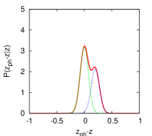
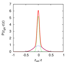
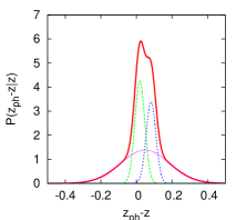
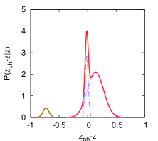
Figure 1.— Examples of photo-z probability distribution $P(z_{\rm ph}|z)$. From left to right, they are two Gaussians with different biases, two Gaussians with different $\sigma_{z}$ values, three Gaussians with parameters randomly generated, and three Gaussians with one being catastrophic. The thick solid lines are the total $P(z_{\rm ph}|z)$, and the thin dotted lines are the individual Gaussians that build up $P(z_{\rm ph}|z)$.

Ma et al. (2006) show that $N_{\rm pz}=31$ between $z=0$ and 3 gives enough freedom to the photo-z parameters to destroy all tomographic information. Since we are giving the photo-z even more freedom by allowing $P(z_{\rm ph}|z)$ to be multiple Gaussians, $N_{\rm pz}=31$ should be large enough. Unless stated otherwise, we use $N_{\rm pz}=31$. Thus, the total number of photo-z parameters is $62N_{g}$.

The observables $n(z_{\rm ph}^{i})$, determined in bins of width $\delta z_{\rm ph}$, need not have the same bin width as the spacing of the $n(z^{i})$ or the photo-z parameters. In fact, they should be more finely spaced. We choose the size of $\delta z_{\rm ph}$ such that further dividing it by two does not lead to anymore information gains. We find that $\delta z_{\rm ph}=0.0125$ is small enough for all the photo-z models explored in this study.

4. Size of the Spectroscopic Calibration Sample

In this section we investigate the size of the spectroscopic calibration sample required to limit photo-z systematics to some desired level. In particular, we are interested in the increased demands that might result from giving the photo-z distribution freedom to depart from a single-Gaussian form. We first demonstrate that, for a fixed fiducial photo-z model, the required calibration size increases with the number of degrees of freedom ($2N_{g}$) that we allow for deviations from the fiducial model. This increase reaches an asymptotic limit with $N_{g}$.

Second, we investigate how the required $N_{\rm spect}$ varies as we allow the fiducial model to assume non-Gaussian shapes. Equations A-9 and A-10 show that in the case of a Gaussian distribution, the $N_{\rm spect}$ required to constrain the photo-z parameters is proportional to the square of the width of the distribution. In the following, we hold the width (defined as the rms) of the fiducial photo-z distributions to be $0.05(1+z)$. Holding this fiducial width fixed means that any variations we see are due only to variations in the shape of the photo-z probability distribution.

We use the error degradations in $w_{\rm a}$ (that is, errors in $w_{\rm a}$ relative to the error with perfect knowledge of the photo-z parameters) as the measure of dark energy degradations. The error degradations in $w_{\rm p}$ are about $30$-$50\%$ lower and follow the same trend as that of $w_{\rm a}$. Roughly speaking, the figure of merit adopted by the Dark Energy Task Force (Albrecht et al., 2006) will degrade as the square of the dark energy degradation used here.

In this section we assume that the $N_{\rm spect}$ total spectroscopic galaxies are selected uniformly in redshift between 0 and 3.

4.1. Dependence on the Number of Gaussians $N_{g}$

The left panel of Figure 2 plots the dark energy degradation versus the size of the spectroscopic calibration sample, when the photo-z error distribution has $N_{g}=1$, $2$, $3$, and $4$. The fiducial biases and dispersions are the same for all component Gaussians. So the fiducial $P(z_{\rm ph}|z)$ is identical in all cases, but with higher $N_{g}$, there is more freedom for deviations from the fiducial. The second, third, and fourth Gaussian components are each fixed to have one-fourth the total normalization of the distribution.

At fixed dark energy degradation, the required size of the calibration sample ($N_{\rm spect}$) increases with the number of Gaussians and reaches an asymptotic value when $N_{g}\approx 4$. When dark energy degradation is 1.5, the $N_{\rm g}=4$ photo-z model requires $\approx 5$ times the calibration sample of the $N_{\rm g}=1$ model.

Another view is that the dark-energy uncertainties will be underestimated if one fits a single-Gaussian model to photo-z distributions that actually require more freedom. For example, assume we obtain $4\times 10^{4}$ spectra, as required to keep dark energy degradation under 1.5 for a single-Gaussian photo-z model. We find, however that the dark energy degradation for $N_{g}=4$ rises above 2.0. So relaxing the Gaussian assumption for photo-z’s inflates the cosmological uncertainties by $\approx 35\%$.

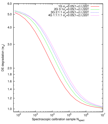
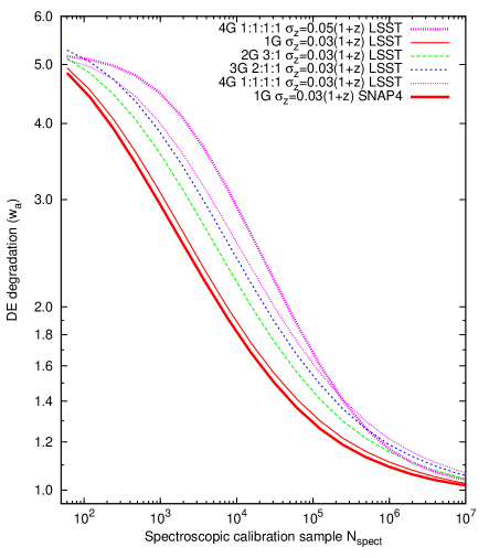
Figure 2.— Left: The $N_{\rm spect}$ requirement for the same fiducial photo-z distribution being modeled using different numbers of Gaussians. These Gaussians differ only by their normalizations, whose ratios are shown in the legend (e.g., “2G 3:1” means a two-Gaussian model with normalization ratio of 3 to 1.). All Gaussian components have fiducial $z_{\rm bias}=0$ and $\sigma_{z}=0.05(1+z)$, so all cases have the same fiducial distribution while the fitted photo-z error distribution gains more freedom. The solid line is for the case of single Gaussian ($N_{g}=1$). Survey specs are LSST-like. Right: Thin lines are the same as those in the left panel but with $\sigma_{z}=0.03(1+z)$. For comparison, the four-Gaussian model in the left panel is plotted as the thick dotted line (magenta). The thick solid line (red) is the single-Gaussian model with SNAP-like survey specs ($f_{\rm sky}=4000$ deg², $\bar{n}^{A}=100$ galaxies arcmin^-2, and $\gamma_{\rm int}=0.22$).

We also note from the left panel of Figure 2 that the dark energy degradation has a characteristic dependence on $N_{\rm spect}$; for $N_{\rm spect}\gtrsim 10^{3}$, the dark energy parameter error scales roughly as $N_{\rm spect}^{1/4}$. When the dark energy degradation reaches $\approx 1.2$, at $N_{\rm spect}=10^{5}$–$10^{6}$, the gains from additional spectra become weaker and a degradation of unity is approached only very slowly. As we vary $N_{g}$, we change the location of this “knee” in the curve, but not the scaling for $N_{\rm spect}$ below the knee. This scaling is not sensitive to either the fiducial photo-z models or survey specs. For example, as shown in the right panel of Figure 2, for a photo-z model with $\sigma_{z}=0.03(1+z)$, the scaling is $N_{\rm spect}^{1/5}$; for a SNAP-like survey with $f_{\rm sky}=4000$ deg², $\bar{n}^{A}=100$ galaxies arcmin^-2, and $\gamma_{\rm int}=0.22$, the scaling is also $N_{\rm spect}^{1/5}$ as shown in the right panel of Figure 2.

The desired spectroscopic survey size $N_{\rm spect}$ will in general depend on the width and shape of the fiducial photo-z distribution, not just $N_{g}$. We next investigate the dependence on the detailed shape of the fiducial distribution.

4.2. Dependence on the Fiducial Photo-z Models

The left panel of Figure 3 shows dark energy degradation versus $N_{\rm spect}$ for several $N_{g}=2$ models, all having fiducial rms width $0.05(1+z)$, but with different fiducial biases and dispersions for the two components. In detail, our study includes fiducial photo-z distributions in which: the component Gaussians have the same biases but different $\sigma_{z}$ values (“2G $\sigma_{z}$ diff” model); the same $\sigma_{z}$ values but different biases (“2G zbias diff”); the same biases and $\sigma_{z}$ values but with normalizations at a 3 to 1 ratio (“2G 3:1”); and 10 models in which the fiducial $z_{\rm{bias;j}}$ and $\sigma_{z;j}$ are randomly assigned while maintaining fixed rms photo-z error (“2G seed xxx” models).

The $N_{\rm spect}$ requirements span a rather large range. For example, at $50\%$ dark energy degradation, most of the photo-z models’ $N_{\rm spect}$ requirement is within a factor of 4 of that of the single-Gaussian model. But some of the models require $40$ times more $N_{\rm spect}$. Three- and four-Gaussian photo-z models exhibit similar behaviors.

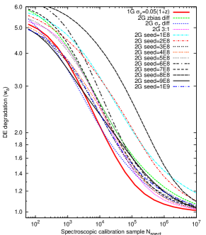
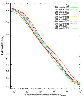
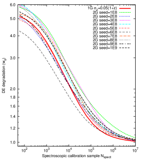
Figure 3.— The $N_{\rm spect}$ requirement for different fiducial photo-z models with $N_{g}=2$, including some with randomly generated fiducial photo-z error distributions. Details of the photo-z models are in § 4.2. Left: Information from the galaxy photo-z distribution $n(z_{\rm ph})$ and the spectroscopic calibration sample are used to constrain the underlying galaxy redshift distribution $n(z)$ and photo-z parameters. Middle: Same as the left panel, except that information from $n(z_{\rm ph})$ is not utilized and $n(z)$ is assumed to be known a priori. Right: Within each of the three $\delta z=1$ intervals, the randomly generated fiducial $z_{\rm bias}$ and $\sigma_{z}$ values increase linearly with $1+z$. The proportionalities are generated randomly. In all three panels, the thick solid red line is for the case of a single Gaussian ($N_{g}=1$).

To understand the wide range of $N_{\rm spect}$ requirements for different photo-z models, we perform the following test. We fix the underlying galaxy redshift ${n(z)}$ and do not use any information from ${n(z_{\rm ph})}$. The resulting $N_{\rm spect}$ requirements for the double-Gaussian photo-z models are shown in the middle panel of Figure 3. At fixed dark energy degradation, the range of $N_{\rm spect}$ requirements is greatly reduced. For example, at $50\%$ dark energy degradation, the $N_{\rm spect}$ requirement is within a factor of 2 of that of the single-Gaussian model. We find similar reduction of the range of $N_{\rm spect}$ requirements in the case of three- and four-Gaussian models. The test shows that the reason for the wide range of $N_{\rm spect}$ requirements for different photo-z models is that $n(z_{\rm ph})$ constrains the underlying galaxy redshift distribution and the photo-z parameters much better in some of the photo-z models than others. It is the redshift knowledge, rather than weak-lensing information itself, that is sensitive to the details of the photo-z probability distribution.

One possible cause of the poor sensitivity in some photo-z models is the rapid variation of photo-z parameters in redshift. The right panel of Figure 3 shows the result of reducing the degree of rapid variation of the photo-z parameters. The range of $N_{\rm spect}$ is reduced to within a factor of 4 of that of the single-Gaussian model as shown in right panel of Figure 3. In detail, we demand that the fiducial photo-z parameter $z_{\rm bias}$ and $\sigma_{z}$ values to be proportional to $1+z$ within each of the three redshift intervals with width $\delta z=1$. The proportionalities are generated randomly. These photo-z models are much smoother than those randomly generated in the left panel of Figure 3. This test shows that $n(z_{\rm ph})$ is less effective in constraining the underlying galaxy redshift distribution and photo-z parameters when the photo-z model is rapidly varying. In reality, photo-z parameters would most likely show smooth variations in redshift. The required calibration sample is expected to be within a factor of a few times that of the single-Gaussian fiducial model.

We point out that multi-Gaussian cases may require fewer spectroscopic calibration galaxies than the single-Gaussian case. As an example, examine the photo-z model with double Gaussians whose $\sigma_{\rm z}$ values are different. Its $N_{\rm spect}$ requirement is shown in Figure 3 (left) using the dotted blue line. Since we keep the width of $P(z_{\rm ph}|z)$ fixed, one of the Gaussians in the double-Gaussian photo-z model is narrower than the width of $P(z_{\rm ph}|z)$ and the other Gaussian is broader. The narrower Gaussian tends to reduce the $N_{\rm spect}$ requirement, while the broader one tends to do exactly the opposite. The outcome of these competing effects could be either a smaller or larger requirement of the calibration sample. For this particular photo-z model, the required $N_{\rm spect}$ crosses that of the single-Gaussian model (shown as the thick solid red curve in Fig 3 left).

We note that the generic behavior $\sigma_{w_{a}}\propto N_{\rm spect}^{0.2-0.25}$ continues to hold for all the fiducial distributions, until the dark energy degradation drops to 1.2–1.3. This inflection typically occurs with a few times $10^{5}$ spectra, for the LSST survey parameters assumed here.

5. Optimizing the Spectroscopic Calibration Sample

So far we have been assuming that the calibration sample is uniformly distributed in redshift. Weak lensing may require more precise photo-z calibration at some redshifts than others. It could be beneficial if we distribute the calibration sample according to lensing sensitivity. Our goal is to find the $N_{\rm spect}^{i}$ that leads to the best dark energy constraints for a fixed spectroscopic observing time $T_{\rm obs}$. This could be modeled as

$$(\mathrm{Uncertainties} {}\mathrm{in\,\,dark\,\,energy\,\,parameters})=$$ (20)

$${}{\it function}(N_{\rm spect}^{i}\,,i=1,2,...)\,,$$

$$\sum_{i=1}N_{\rm spect}^{i}cost(z^{i})=T_{\rm obs}\,,$$ (21)

where $cost(z^{i})$ is the time it takes to obtain the spectrum of a galaxy at redshift $z^{i}$. This is a constrained nonlinear optimization problem. To calculate the function in equation 20, we first calculate the Fisher matrices ${\rm F}^{\rm lens}$ and ${\rm F}^{n(z_{\rm ph})}$ for the presumed survey. Then for each trial set of $N^{i}_{\rm spect}$, we calculate $F^{\rm spect}$ using equation 14, sum the Fisher matrices, and forecast the dark energy uncertainties. As to the constrain equation (21), we need to know the cost function. For illustrative purposes, we assume $cost(z^{i})$ is a constant.

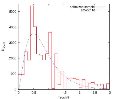
Figure 4.— Histogram: Optimal $N_{\rm spect}$ distribution in redshift for single-Gaussian model. Dark energy degradation is $56\%$ if this sample is distributed uniformly in redshift. The $N_{\rm spect}$ distribution in this figure lowers dark energy degradation to $38\%$, which would require $69,000$ galaxy spectra to calibrate if the distribution is flat in redshift. Blue dashed line: Smooth fit to the histogram. The dark energy degradation is $44\%$ if this calibration sample is used. For both the histogram and the smooth fit, the calibration sample has 37,500 galaxies.

As an example we choose a calibration sample of 37,500 galaxies and assume a single-Gaussian photo-z model. If this calibration sample is uniformly distributed in redshift, dark energy degradation is $56\%$. If instead we use a downhill simplex method to find the spectroscopic redshift sampling distribution that minimizes the dark energy uncertainties for a fixed total number of redshifts, we obtain the distribution shown as the histogram in Figure 4. The optimized redshift sampling lowers the dark energy degradation to $38\%$. That is a $18\%$ gain in dark energy precision at fixed investment of spectroscopy time. From a different prospective, to reach $38\%$ dark energy degradation with a uniformly distributed calibration sample, $69,000$ galaxy spectra are required. So optimization saves $46\%$ of the spectroscopic observing time for fixed cosmological degradation. Multi-Gaussian photo-z models exhibit very similar behaviors.

We do not know exactly why the optimized calibration sample distribution is not very smooth. It would be rather difficult to plan the observation to match this distribution. Fortunately, a smooth distribution like the one shown using the blue dashed line in Figure 4 produces $44\%$ dark energy degradation, which is a moderate improvement over the uniform case.

6. Conclusion and Discussion

We explore the dependence of cosmological parameter uncertainties in WL power-spectrum tomography on the size of the spectroscopic sample for the calibration of photometric redshifts. We present a formula that is valid for arbitrary parameterizations of the photo-z error distribution and then apply this to a multi-Gaussian model to see whether previous works’ assumptions of simple Gaussian photo-z errors were yielding accurate results.

Indeed, we find that the required $N_{\rm spect}$ under the simple Gaussian model is increased $\approx 4$ times when we allow more freedom in the shape of the core of the photo-z distribution. Fortunately, there appears to be an asymptotic upper limit as we add more photo-z degrees of freedom.

We also find a generic behavior $d\log\sigma/d\log N_{\rm spect}=$ 0.20–0.25, where $\sigma$ is the uncertainty in a dark energy parameter, in the regime where $\sigma$ is degraded 1.2–5 times compared to the case of perfect knowledge of the photo-z distribution. Hence, the fourfold increase in required $N_{\rm spect}$ from relaxing the Gaussian assumption is equivalent to a $\approx 1.3$ times degradation in $\sigma$ at fixed $N_{\rm spect}$.

The exact value of dark energy degradation versus $N_{\rm spect}$ depends significantly on the shape of the fiducial distribution, even when the total rms photo-z error is held fixed. For the case of the LSST survey with rms photo-z error $0.05(1+z)$, we find that the “knee” at a dark energy degradation of 1.2–1.3 occurs in the range $N_{\rm spect}\approx 10^{5}$–$10^{6}$.

For photo-z models described by nondegenerate Gaussians, the size of the calibration sample varies by as much as 40 times among the 14 models studied. Most of the variation is caused by the different ability of the galaxy photo-z distribution $n(z_{\rm ph})$ to constrain the underlying galaxy redshift distribution and the photo-z probability distribution. These photo-z models whose parameters vary rapidly in redshift are the ones that are least constrained. In reality, photo-z parameters are expected to be smoothly varying in redshift. The $N_{\rm spect}$ requirement would be only a factor of a few from that of the single-Gaussian fiducial distribution.

Finally, we show that the size of the calibration sample can be effectively reduced by optimization. In a simple example, an optimized calibration sample of 37,500 redshifts was able to reach the same dark energy degradation as a sample of 69,000 galaxies uniformly distributed in redshift.

We restrict this study to the effect of the core of the photo-z distributions. Catastrophic photo-z errors could potentially be very damaging. The methodology provided in this study is applicable to study the effect of catastrophic photo-z errors. We leave this to future work.

The methodology we use assumes that the spectroscopic survey is a fair sample of the photo-z error distribution and is the only information available on the photo-z error distribution. Since we have used a Fisher matrix technique, no photo-z estimation method, regardless of technique (neural net, template fitting, etc.) can surpass our forecasts under these conditions.

The calibration’s success depends crucially on the spectroscopic redshifts being drawn without bias from the redshift distribution of the photometric sample it represents. The survey strategy must be carefully formulated to make sure that this occurs. Differential incompleteness between, say, red and blue galaxies or redshift “deserts”, must be avoided. This has not been achieved by any large redshift survey beyond $z\approx 0.5$ to date.

It may be possible to constrain $P(z_{\rm ph}|z)$ by other means in the absence of a fair spectroscopic sample of the size we specify. One could invoke astrophysical assumptions, namely, that the spectra of faint galaxies are identical to those of brighter galaxies, in an attempt to bootstrap a fair bright sample into a calibration for fainter galaxies. Another suggestion (Schneider et al. (2006); J. Newman, private communication) is that the photometric sample be cross-correlated with an incomplete spectroscopic sample to infer the redshift distribution of the former. It remains to be seen, however, whether these techniques can attain the accuracy needed to supplant a direct fair sample of $>10^{5}$ spectra. This would require some a priori bounds on the evolution of galaxy spectra and the clustering correlation coefficients of different classes of galaxies. We look forward to future progress in these techniques, keeping in mind that the demands for precision cosmology from WL tomography are much more severe than the demands that galaxy evolution studies typically place on photometric redshift systems.

Appendix: Derivation of Equation 14

If one draws $N$ events from a sample with probability distribution function $P(x;{\mbox{\boldmath$\theta$}})$, where the components of $\theta$ are the parameters specifying the distribution and $x$ is the variable whose probability distribution is under consideration, what are the constraints on the parameters $\theta$?

Let us first divide $x$ into small bins and label the width of the bins as $\Delta x_{i}$. The number of events that fall in the $i$th bin is Poisson distributed with mean $\bar{N_{i}}=NP(x_{i};{\mbox{\boldmath$\theta$}})\Delta x_{i}$. The likelihood function can be expressed as

$$L\propto\prod_{i}{\exp(-\bar{N_{i}})\bar{N_{i}}^{N_{i}}\over{N_{i}!}}\,,$$ (A-1)

and the natural logarithm of $L$ is,

$${\mathcal{L}}\equiv-lnL=\sum_{i}\bar{N_{i}}-N_{i}ln\bar{N_{i}}+lnN_{i}!+const\,\,.$$ (A-2)

The derivatives of ${\mathcal{L}}$ with respect to the model parameters $\theta$ are

$${\partial{\mathcal{L}}\over{\partial\theta_{\mu}}}=\sum_{i}\left(1-{N_{i}\over{\bar{N_{i}}}}\right){\partial{\bar{N_{i}}}\over{\partial\theta_{\mu}}}\,\,\,\,\,\,\,\,\,and,$$ (A-3)

$${\partial^{2}{\mathcal{L}}\over{\partial\theta_{\mu}\partial\theta_{\nu}}} = {}\sum_{i}\left[{N_{i}\over{\bar{N_{i}}^{2}}}{\partial{\bar{N_{i}}}\over{\partial\theta_{\mu}}}{\partial{\bar{N_{i}}}\over{\partial\theta_{\nu}}}\right.$$ (A-4)

$${}\left.+\left(1-{N_{i}\over{\bar{N_{i}}}}\right){\partial^{2}{\bar{N_{i}}}\over{\partial\theta_{\mu}\partial\theta_{\nu}}}\right]\,.$$

The Fisher matrix is,

$$F_{\mu\nu} \equiv {}\left<{\partial^{2}{\mathcal{L}}\over{\partial\theta_{\mu}\partial\theta_{\nu}}}\right>=\sum_{i}{1\over{\bar{N_{i}}}}{\partial{\bar{N_{i}}}\over{\partial\theta_{\mu}}}{\partial{\bar{N_{i}}}\over{\partial\theta_{\nu}}}$$ (A-5)

$$= \sum_{i}{N\Delta x_{i}\over{P(x_{i};{{\mbox{\boldmath$\theta$}}})}}{\partial{P(x_{i};{{\mbox{\boldmath$\theta$}}})}\over{\partial\theta_{\mu}}}{\partial{P(x_{i};{{\mbox{\boldmath$\theta$}}})}\over{\partial\theta_{\nu}}}$$

$$= N\int dx{1\over{P(x;{{\mbox{\boldmath$\theta$}}})}}{\partial{P(x;{{\mbox{\boldmath$\theta$}}})}\over{\partial\theta_{\mu}}}{\partial{P(x;{{\mbox{\boldmath$\theta$}}})}\over{\partial\theta_{\nu}}}\,.$$

In the special case where $P(x;{{\mbox{\boldmath$\theta$}}})$ is a Gaussian with mean $\mu$ and spread $\sigma$,

$$P(x;\mu,\sigma)={1\over{\sqrt{2\pi}\sigma}}\exp\left[-{(x-\mu)^{2}\over{2\sigma^{2}}}\right]\,,$$ (A-6)

we have

$${\partial P\over{\partial\mu}}={x-\mu\over{\sigma^{2}}}P\,\,\,\,\,\,\,\,\,and,$$ (A-7)

$${\partial P\over{\partial\sigma}}=-{P\over{\sigma}}+{(x-\mu)^{2}\over{\sigma^{3}}}P\,.$$ (A-8)

Plugging these results into equation A-5 gives us

$$F_{\mu\mu}=N\int_{-\infty}^{\infty}dx{(x-\mu)^{2}\over{\sigma^{4}}}P={N\over{\sigma^{2}}}\,\,\,\,\,\,\,\,\,and,$$ (A-9)

$$F_{\sigma\sigma}=N\int_{-\infty}^{\infty}dxP\left[{(x-\mu)^{2}\over{\sigma^{3}}}-{1\over{\sigma}}\right]^{2}={2N\over{\sigma^{2}}}\,.$$ (A-10)

Note that $F_{\mu\sigma}=0$ since the integral only involves odd powers of $x-\mu$.

References

- Abdalla et al. (2007) Abdalla, F.B., Amara, A., Capak, P., Cypriano, E.S., Lahav, O., & Rhodes, J., 2007, astro-ph/0705.1437
- Albrecht et al. (2006) Albrecht, A., Bernstein G., & Cahn, R. et al., 2006, astro-ph/0609591
- Amara, & Refregier (2007) Amara, A., & Refregier, A., 2007, MNRAS, 381, 1018 (astro-ph/0610127)
- Bernstein & Jarvis (2002) Bernstein, G. & Jarvis, B. 2002, AJ, 583, 123
- Bridle & King (2007) Bridle, S., & King, L., 2007, astro-ph/0705.0166
- Dahlen et al. (2007) Dahlen, T., Mobasher, B., & Jouvel, S. et al., 2007, astro-ph/0710.5532
- Dodelson et al. (2006) Dodelson, S., Shapiro, C., & White, M. 2006, Phys. Rev. D73, 023009 (astro-ph/0508296)
- Dodelson & Zhang (2005) Dodelson, S. & Zhang, P. 2005, Phys. Rev. D72, 083001 (astro-ph/0501063)
- Eisenstein & Hu (1999) Eisenstein, D.J. & Hu, W. 1999, ApJ, 511, 5
- Francis et al. (2007) Francis, M., Lewis, G., & Linder E., 2007, MNRAS, 380, 1079 (astro-ph/0704.0312)
- Hagan, Ma & Kravtsov (2005) Hagan, B., Ma C-P. & Kravtsov A. 2005, ApJ, 633, 537-541 (astro-ph/0504557)
- Heymans et al. (2006) Heymans, C., Waerbeke, L.V., Bacon, D., Berge, J. et al, 2006, MNRAS, 368, 1323-1339 (astro-ph/0506112)
- Heitmann et al. (2005) Heitmann, K., Ricker, P. M., Warren, M. S., Habib, S., 2005, ApJS, 160, 28 (astro-ph/0411795)
- Hirata & Seljak (2003) Hirata, C. & Seljak, U. 2003, MNRAS, 343, 459
- Hoekstra (2004) Hoekstra, H. 2004, MNRAS, 347, 1337
- Hu (1999) Hu, W., 1999, ApJ, 522, L21
- Hu (2002) Hu, W. 2002, Phys. Rev. D, 65, 023003
- Huterer (2002) Huterer, D., 2002, Phys. Rev. D, 65, 063001
- Huterer & Takada (2005) Huterer, D. & Takada, M. 2005, Astropart. Phys., 23, 369
- Huterer et al. (2006) Huterer, D., Takada, M., Bernstein, G & Jain, B. 2006, MNRAS, 366, 101-114 (astro-ph/0506030)
- Huterer & White (2005) Huterer, D., & White, M. 2005, Phys.Rev. D72, 043002 (astro-ph/0501451)
- Jain et al. (2007) Jain, B., Connolly, A., & Takada, M., 2007, J. Cosmol. Astropart. Phys., 03, 013 (astro-ph/0609338)
- Jarvis & Jain (2004) Jarvis, M. & Jain, B. 2004, astro-ph/0412234
- Jing et al. (2006) Jing, Y.P., Zhang, P., Lin, W.P. et al., 2006, ApJ, 640, L119 (astro-ph/0512426)
- Kaiser (1992) Kaiser, N. 1992, ApJ, 388, 272
- Kaiser (1998) Kaiser, N. 1998, ApJ, 498, 26
- Linder & White (2005) Linder, E., & White, M., 2005, Phys. Rev. D72, 061304 (astro-ph/0508401)
- Ma et al. (2006) Ma, Z., Hu, W. & Huterer, D., 2006, ApJ, 636, 21 (astro-ph/0506614)
- Ma (2006) Ma, Z., 2006, ApJ, 665, 887-898 (astro-ph/0610213)
- Massey et al. (2007) Massey, R., Heymans, C., Berge, J., Bernstein, G. et al., 2007, MNRAS, 376, 13-38 (astro-ph/0608643)
- Nakajima & Bernstein (2007) Nakajima, R., & Bernstein, G., 2007, AJ, 133, 1763 (astro-ph/0607062)
- Oyaizu et al. (2007) Oyaizu, H., Lima, M., & Cunha, C. et al., 2007, astro-ph/0711.0926
- Peacock & Dodds (1996) Peacock, J.A. & Dodds, S.J. 1996, MNRAS, 280, L19
- Rudd et al. (2008) Rudd, D., Zentner, A. & Kravtsov, A., 2008, ApJ, 672, 19 (astro-ph/0703741)
- Schneider et al. (2006) Schneider, M., Knox, L., Zhan, H., & Connolly, A., 2006, ApJ, 651, 14 (astro-ph/0606098)
- Shapiro & Cooray (2006) Shapiro, C., & Cooray, A., 2006, JCAP, 0603, 007 (astro-ph/0601226)
- Spergel et al. (2003) Spergel, D.N. 2003, ApJ, 148, 175
- Stabenau et al. (2007) Stabenau, H. F., Connolly, A., & Jain, B., 2007, astro-ph/0712.1594
- Vale et al. (2004) Vale, C., Hoekstra, H., van Waerbeke, L. & White, M. 2004, ApJ, 613, L1
- Vale & White (2003) Vale, C. & White, M., 2003, ApJ, 592, 699
- White (2004) White, M., 2004, Astroparticle. Phys., 22, 211
- White (2005) White, M., 2005, Astroparticle. Phys., 23, 349
- White & Vale (2004) White, M. & Vale, C., 2004, Astroparticle. Phys., 22, 19
- Wittman et al. (2007) Wittman, D., Riechers, P., & Margoniner V.E., 2007, ApJ, 671, L109, (astro-ph/0709.3330)
- Zentner et al. (2008) Zentner, A., Rudd, D., & Hu, W., 2008, Phys. Rev. D, 77, 043507 (astro-ph/0709.4029)
- Zhan & Knox (2004) Zhan, H. & Knox, L. 2004, ApJ, 616, L75