Photometric redshifts with surface brightness priors

Abstract

We use galaxy surface brightness as prior information to improve photometric redshift estimation. We apply our template-based photo-z method to imaging data from the ground-based VVDS survey and the space-based GOODS field from HST, and use spectroscopic redshifts to test our photo-z’s for different galaxy types and redshifts. We find that the surface brightness prior eliminates a large fraction of outliers by lifting the degeneracy between the Lyman and 4000 Ångstrom breaks. Bias and scatter are improved by about a factor of two with the prior in each redshift bin in the range $0.4<z<1.3$, for both the ground and space data. Ongoing and planned surveys from the ground and space will benefit provided that care is taken in measurements of galaxy sizes and in the application of the prior. We discuss the image quality and signal-to-noise requirements that enable the surface brightness prior to be successfully applied.

1 Introduction

Photometric redshifts (“photo-z’s”) are a tool for obtaining redshift and type information for galaxies for which broadband photometric colors are available rather than spectroscopic data. Generally, this technique is used to study populations of galaxies when the observational cost of obtaining spectra for these galaxies would be prohibitive. With the advent of wide field imaging surveys, photo-z estimation has become an indispensable part of cosmological surveys. With imaging in three to five optical bands, ongoing and planned surveys aim to get photo-z’s over hundreds or thousands of square degrees of sky. With the redshift and sky positions, surveys such as DES, KiDS, LSST, and Pan-STARRS plan to use galaxy clusters, galaxy clustering and gravitational lensing as probes of dark energy and other cosmological issues. The techniques and accuracy of photo-z’s have become an area of active study since they play a critical role in deriving cosmological information from imaging surveys.

Recently, two main approaches have been used to obtain photo-z’s: empirical fitting and template fitting. In the former, a neural network, polynomial function, or other empirical relation is trained using a subsample of galaxies with known (spectroscopic) redshifts, and then applied to the larger sample (Connolly et al., 1995; Vanzella et al., 2004; Firth et al., 2003; Brodwin et al., 2006; Collister et al., 2007; Oyaizu et al., 2008; D’Abrusco et al., 2007; Li et al., 2006; Abdalla et al., 2007; Banerji et al., 2008). In the template-fitting method, first a library of theoretical or empirical spectral energy distributions (“SEDs”) are generated, and then they are fit to the observed colors of galaxies, where the redshift is a parameter that is fit (Arnouts et al., 1999; Benitez, 2000; Bolzonella et al., 2000; Babbedge et al., 2004; Ilbert et al., 2006; Brodwin et al., 2006; Feldmann et al., 2006; Mobasher et al., 2007; Brodwin et al., 2006; Margoniner & Wittman, 2007; Wittman et al., 2007). As in the training set approach, a subsample of galaxies with spectroscopic redshifts can be used to help calibrate this procedure. In this study we use a template-fitting method, which makes use of a library of galaxy templates (Bruzual A. & Charlot, 1993; Bruzual & Charlot, 2003), to predict the colors of galaxies through a series of optical and infrared passbands. In principle the idea is simple: given an observed galaxy, compute the redshift $z$ that makes each template $T$ match the observed colors most closely, and then choose the best fit $(T,z)$ pair.

The reality is more difficult. With only a limited number of colors, it’s often impossible to tell whether a set of observed colors better matches one template which is at high $z$, or another at low $z$. This is known as the “color-redshift degeneracy,” and occurs because a red galaxy template at low redshift and a blue galaxy template at high redshift can look the same in a given set of filters. For the same reason, accurately determining the rest-frame color of a galaxy (the “$k$-correction”) is difficult: intrinsic astrophysical variations and evolution broaden scatter in the color-$z$ relation, and the effect increases at higher redshift. With this paper we address the question of how to break this degeneracy. The most widely used method uses empirically measured apparent magnitude–redshift distributions (see e.g. Benitez, 2000); in this paper, we introduce a new and complementary approach to breaking the color-redshift degeneracy using the surface brightness (SB), which is the luminosity of an object per unit surface area. We will show that the SB is able to provide a strong constraint on galaxy redshifts, which should remain intact even for faint samples, and that this will not be the case for the magnitude prior. In order to incorporate prior statistical information about the galaxies under study into the redshift estimate in a consistent way, we use the Bayesian approach first introduced by Benitez (2000).

Throughout this paper we use the AB magnitude system.

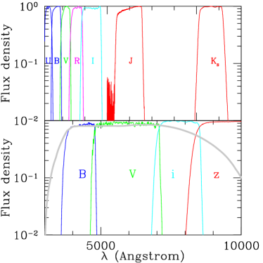
Figure 1: Flux density vs wavelength for the filters used in the GOODS and VVDS surveys. The ACS filters used are F435W (Johnson $B$), F606W (Broad $V$), F775W (SDSS $i$), and F850LP (SDSS $z$). The VVDS filters are Mould $U$, $B$, $V$, $R$, and $I$ filters, as well as ESO/WFI $J$ and $K_{s}$ filters. The detector response function for the ACS is indicated on the lower plot.

2 Bayesian Photometric Redshifts

Our goal is to find, for each galaxy, the 2-D posterior distribution $P(z,T|{\bf C},{\bf O})$, where $z$ is the redshift of the galaxy, $T$ is the “template parameter,” which is a discrete variable corresponding to the galaxy type in our template library, ${\bf C}$ is the vector of fluxes from the data, and ${\bf O}$ is a vector of observables independent of the fluxes ${\bf C}$ for each galaxy. ${\bf O}$ could be any set of observables, e.g. size, brightness, morphology, environment. In the current paper we consider $I$-band apparent magnitude and apparent surface brightness. Using Bayes’ theorem and the definition of conditional probability, we can write

$$P(z,T|{\bf C},{\bf O})=\frac{P({\bf C},{\bf O},z,T)}{P({\bf C},{\bf O})}=\frac{P({\bf C}|{\bf O},z,T)P({\bf O},z,T)}{P({\bf O})P({\bf C})},$$ (1)

because we make the approximation that ${\bf O}$ and ${\bf C}$ are independent. By the same token, we can write $P({\bf C}|{\bf O},z,T)=P({\bf C}|z,T)$, and then since $P(z,T,{\bf O})/P({\bf O})=P(z,T|{\bf O}),$

$$P(z,T|{\bf C},{\bf O})=\frac{P({\bf C}|z,T)P(z,T|{\bf O})}{P({\bf C})}.$$ (2)

This is the equation on which our work is based. The posterior distribution $P(z,T|{\bf C},{\bf O})$ is given in terms of the likelihood function $P({\bf C}|z,T)$ and the prior distribution $P(z,T|{\bf O})$; the prior encompasses all the prior knowledge we wish to use about galaxy morphology, evolution, environment, brightness, etc. Once the posterior distribution is determined, all the quantities of interest can be calculated; ideally, any study that wishes to make use of photo-z information would use the full $P(z,T|{\bf C},{\bf O})$ directly. For the sake of simplicity, we evaluate the performance of our estimator using the mode of $P(z,T|{\bf C},{\bf O})$, which is the “best” redshift

$$z_{p}\equiv z(P=P_{\rm max}).$$ (3)

We can also compute the marginalized redshift estimate given by

$$\langle z\rangle=\frac{\int dTdz\,zP(z,T|{\bf C},{\bf O})}{\int dTdz\,P(z,T|{\bf C},{\bf O})},$$ (4)

and the variance

$$\langle z^{2}\rangle-\langle z\rangle^{2}=\frac{\int dTdz\,z^{2}P(z,T|{\bf C},{\bf O})}{\int dTdz\,P(z,T|{\bf C},{\bf O})}-\langle z\rangle^{2}.$$ (5)

As we will show, we find that $P(z,T|{\bf C})$ is typically multimodal with one minimum in $\chi^{2}$ close to the spectroscopic redshift and one or more “false” minima at other redshifts. Using $z_{p}$ from Eq. (3) as the redshift estimator means that, without a prior, the algorithm can often generate a large error by choosing the estimate from one of the false minima. Including a prior deweights those minima and reduces the impact of the outliers (often referred to as “catastrophic” outliers), greatly improving the accuracy of the $z_{p}$ estimate. Ideally, however, any study using photo-z information should use the full posterior distribution $P(z,T|{\bf C},{\bf O})$ in its analysis.

3 Template Fitting

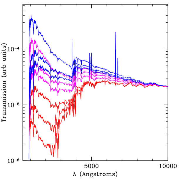
Figure 2: Galaxy templates (GISSEL Bruzual A. & Charlot, 1993; Bruzual & Charlot, 2003) transmission vs $\lambda$, overplotted and normalized to the same value at 10000 Å. The templates on the bottom, shown in red, are the reddest and oldest galaxy populations, while those toward the top are bluer and younger; the ages range from 14 Gyr ($T=0$) to 50 Myr ($T=9$). Convolution with the survey filters flattens out the emission lines, while the 4000 Å and Lyman breaks are still pronounced, which are the primary features of the galaxy spectra that constrain photo-z’s.

In order to calculate the likelihood function $P({\bf C}|z,T)$, we initially model the colors of galaxies as a function of redshift. We use the simple stellar population models from the GISSEL (Galaxy Isochrone Synthesis Spectral Evolution Library) spectral synthesis package (Bruzual A. & Charlot, 1993; Bruzual & Charlot, 2003) to derive a set of spectral energy distributions with ages from 50 Myr to 15 Gyrs. We parameterize the galaxy type as a one dimensional sequence, $T$, that expresses the age of the spectrum with $T=9$ for galaxies with ages of 50 Myr through to $T=0$ for galaxies of age 15 Gyr. All SEDs are convolved with a set of filter response functions taken from the GOODS (Giavalisco et al., 2004) and VVDS (Le Fèvre et al., 2004b) surveys to model the color as a function of redshift over the redshift interval $0<z<4$ (see Figs. 1 and 2). All input spectra are corrected for attenuation due to the intergalactic medium (Madau, 1995). We make no account for evolution in the SEDs as a function of redshift nor do we train the spectral models to correct for uncertainties within the photometric zero-points of the observed data; instead we choose a largely equivalent, and simpler, procedure of fitting a correction to the bias on the calibration sample for use on the (separate) test sample.

Given a model of galaxy colors as a function of redshift and spectral type, $G_{i}(z,T)$, whose values are the flux in the $i^{\rm th}$ band for a given template $T$ and redshift $z$ we then calculate, for each galaxy,

$$\chi^{2}(z,T)=\sum_{i}(C_{i}-\alpha G_{i}(z,T))^{2}/\sigma_{i}^{2},$$ (6)

where $P({\bf C}|z,T)\equiv\exp(-\chi^{2}(z,T)/2)$, $C_{i}$ are the observed fluxes, $\sigma_{i}$ the photometric uncertainties and $\alpha$ is a scale factor that is a free parameter for each galaxy. The scale factor, $\alpha$, means that the template fitting procedure by itself does not take into account the overall brightness of a galaxy, but only its colors. Since we do not have an accurate way to estimate the true error in our template fitting procedure, once we have calculated the full 2-D likelihood function $P({\bf C}|z,T)$, we scale the errors on the measured ${\bf C}$ so that $\chi_{\rm min}(z,T)=1$. Once we have determined the prior distribution $P(z,T|{\bf O})$, we merely have to multiply the two distributions to get the desired posterior distribution. We address how the priors are generated in detail in the next section.

For the current work we utilize the galaxy catalogs from the GOODS and VVDS redshift surveys. For the GOODS data we utilize the $B,V,i,z$ photometric passbands and for the VVDS the $U,B,V,R,I,J,K_{s}$ passbands (see Fig. 1).

4 Priors

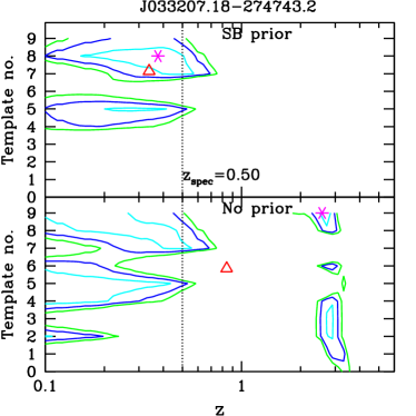
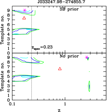
Figure 3: The two panels contain $1-$ (cyan), $2-$ (blue), and $3-\sigma$ (green) probability contours for the two galaxies in Fig. 4. Each galaxy has a multiply-peaked $P(z,T)$ distribution where the template fitting approach fails to select the correct peak without a prior; the red triangle and magenta asterisk marks denote the values of $\langle z\rangle$ and $z(\chi=\chi_{\rm min})$, respectively. For each galaxy, the upper panel shows how the SB prior breaks the degeneracy by eliminating the inaccurate high-redshift maximum, moving both $\langle z\rangle$ and $z_{\rm min}$ closer to the measured spectroscopic redshift, denoted by the dashed line.

The choice of prior $P(z,T|{\bf O})$ is key to a successful template-based photo-z study. The typical failure mode for a template-based photo-z code comes in the form of a multimodal probability distribution, where there is one peak at or near the correct redshift, but at least one other false peak in $(z,T)$-space (see Figs. 3 and 4). The astrophysical origin of these multiple peaks in $(z,T)$-space (and in fact the ability for photometric redshifts to perform as well as they do) comes from the Lyman (1216 Å) and Balmer (4000 Å) breaks in galaxy spectra. The transition of these breaks through a set of filters as a function of redshift provides the change in galaxy color that all photometric redshift techniques key into. If our photometric observations are sufficient to measure the galaxy flux for both breaks then the templates usually have the power to determine the galaxy redshift unambiguously, and there is no degeneracy. This is often not the case for optical surveys. For example, the GOODS survey filters cover the range of approx. 3700–10000 Å, so the Lyman break is only observable for galaxies with $3<z<6$, and the 4000 Å break should be observable for galaxies with $z<1.5$. With only sufficient spectral range to identify a break in the spectrum, but not to classify which break it corresponds to, the template fitting procedure will produce multiple peaks in the $P(z,T)$ distribution. The VVDS adds the infrared filters ($J$ and $K_{s}$ bands) which should help identify the 4000 Å break out to higher redshifts and, therefore, disambiguate the spectral breaks; however, at the depth of the $I$-band selected and $I<24$ magnitude limited sample the infrared observations do not have sufficient signal-to-noise to constrain the infrared colors. In the surveys under study, there are almost no non-QSO/AGN galaxies above $z=2$ that have spectra which meet our quality criterion, so most of the information available to our template fits comes from the 4000 Å break.

In the following subsections we examine how two different methods can break this degeneracy: first, our approach using an empirically-measured SB($z$) relation, and then a widely-used method using the apparent magnitude.

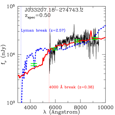
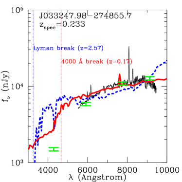
Figure 4: Flux vs wavelength for the two degenerate galaxies shown in Fig. 3. The black curve is the high-resolution spectrum of the galaxy, the dashed blue and solid red curves are the template fits at high and low redshift, respectively, and the green bars are the observations in the broad band filters. The Lyman and 4000 Å breaks are shown by dashed lines. For each galaxy, a $P(z,T)$ distribution is computed by fitting the templates to the observed galaxy colors. However, without prior information, it is nearly impossible to tell which break is present in the spectrum, and therefore, whether the galaxy is at high or low redshift.

4.1 Surface Brightness Prior

4.1.1 Tolman Test

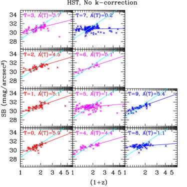
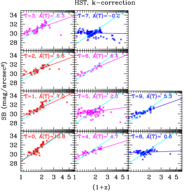
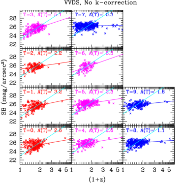
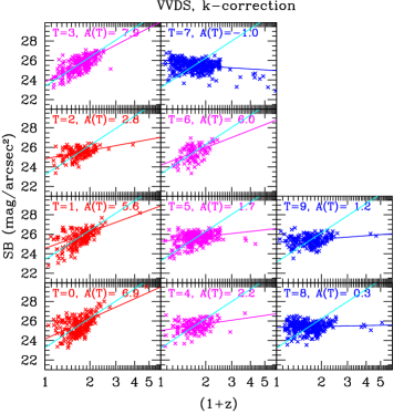
Figure 5: Surface brightness (SB) as a function of spectroscopic redshift, from space and from the ground, with and without magnitude $k$-correction derived from the spectroscopic redshift $z_{s}$ and best-fit template. The panels are labeled by galaxy type (see Fig. 2) and best fit slope of the SB-$\log(1+z)$ relation (see Eq. (9)). When observed from space, the passively-evolving red galaxies are close to the $(1+z)^{-4}$ power law predicted by Eq. (8), shown by the cyan line in each panel. Because the blue galaxies evolve with $z$, they have a shallower slope; this effect becomes more dramatic when $k$-corrections are considered. No attempt has been made to compensate for the larger seeing in VVDS.

In this section, we consider the performance of using SB to break the color-redshift degeneracy. The use of SB in constraining photo-z’s has been proposed a number of times, for example, in the “$\mu$-PhotoZ” method (Kurtz et al., 2007), which is calibrated with the SDSS. The authors use one-color photometry and surface brightness to get photometric redshifts for very red galaxies with $z<0.8$. While their method works well the reddest 10–20% of galaxies, the constraints worsen for bluer types, and thus it is probably not suitable for a general photo-z survey. The SB was also used in Wray & Gunn (2008) as part of a larger framework to improve photo-z’s for a low redshift sample of SDSS galaxies.

The surface brightness (SB) of a galaxy is defined (in units of mag/arcsec²) as:

$${\rm SB}=m+2.5\log{A},$$ (7)

where $m$ is the $I$-band magnitude and $A$ is the angular area. The SB increases as the galaxy gets brighter and smaller. If we let $\chi(z)$ be the comoving distance to redshift $z$, and recall that $m\sim 2.5\log{[\chi^{2}(z)(1+z)^{2}]}$ and $\log{A}\sim\log{[\chi^{-2}(z)(1+z)^{2}]}$, then neglecting $k$-correction, one can plug in to Eq. (7) and derive the evolution of the SB with redshift:

$${\rm SB}(z)=10\log{(1+z)}+{\rm const.}$$ (8)

Equivalently, in flux units we get ${\rm SB}(z)\propto(1+z)^{-4}$. This is how we would expect the SB to behave in an expanding universe for passively evolving galaxies for which there is no magnitude or size evolution with $z$. An interesting point is that ${\rm SB}(z)$ has no explicit dependence on the cosmology; in particular it is independent of the luminosity or angular diameter distances, unlike the magnitude-redshift relation. In fact, the SB($z$) relation has been used to test the hypothesis that the universe is expanding, which is known as the “Tolman test” (Tolman, 1930, 1934; Lubin & Sandage, 2001). Instead of using the expected surface brightness-redshift relation to test whether the universe is expanding, we use SB($z$) to constrain galaxy redshifts.

Just as in Lubin & Sandage (2001), our galaxy sample does not universally follow the simple law given in Eq. (8), because populations of galaxies evolve differently with redshift. The galaxy template library (see Bruzual A. & Charlot, 1993; Bruzual & Charlot, 2003, and Fig. 2) enables us to assign spectral types to each galaxy. We can, therefore, attempt to derive the magnitude $k$-correction for each galaxy using its best fit spectral template and estimate of the redshift. Fig. 5 shows the SB($z$) relation for each galaxy type in our datasets, using the spectroscopic redshift information for the $k$-correction. We can see that, in the panels with $k$-correction, the redder galaxies are evolving more passively and hence closer to the $(1+z)^{-4}$ slope, while the bluer galaxies are actively evolving in such a way that their SB doesn’t change substantially with redshift; from this we infer that there must be significant evolution effects that cause intermediate and blue galaxies at higher redshift to be brighter and/or smaller than passive evolution would indicate. Although they are constrained to lower redshifts ($z<0.8$), we can see similar behavior in Fig. 3 of Kurtz et al. (2007), where the lower left panel, containing the 10% reddest galaxies, follows the expected ${\rm SB}\propto(1+z)^{-4}$ relation most closely, with the strength of the SB($z$) correlation decreasing as bluer deciles are considered.

In the plots with $k$-corrections, the measured slopes are steeper for red galaxies; however, we use the non-$k$-corrected SB to determine $P(z,T|{\rm SB})$. The reason for this is that the effect of $k$-correction is to remove the magnitude evolution with $z$, but the templates already provide this information, so once we have a best-fit template we don’t gain anything from explicitly $k$-correcting; in fact, it results in a larger scatter in SB($z$), because the uncertainties in the k-corrections derived from photometric redshifts increase the scatter in the SB-redshift relation (due to the “catastrophic errors”). The $k$-corrected plots in Fig. 5 have a small scatter because they have used the spectroscopic redshift in order to determine the $k$-correction, i.e. they use extra information that the photo-z procedure doesn’t have.

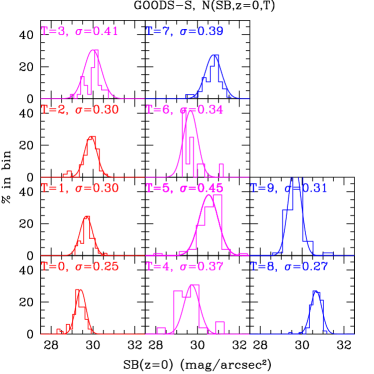
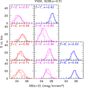
Figure 6: $N({\rm SB},z=0,T)$ with $2\sigma$-clipped Gaussian fits for the GOODS-S and VVDS datasets. Using the fit from Eq. 9 we have shifted the galaxy population in each template bin to $z=0$ and plotted the resulting distribution.

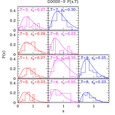
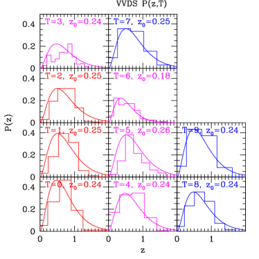
Figure 7: Histograms of $P(z,T)$ for GOODS-S and VVDS datasets. The solid curves are exponential fits: $P(z,T)=(z^{2}/z_{0}^{3}(T))\exp{[-z/z_{0}(T)]}$; the parameter $z_{0}(T)$ is fit separately for each type.

4.1.2 Calibration

We calibrate the SB prior via the following procedure: first, we bin our galaxies into types $T$; each galaxy in the calibration sample has a spectroscopic redshift $z_{s}$ and a measured (non-$k$-corrected) surface brightness ${\rm SB}_{\rm obs}$ (computed using Eq. (7) from the $I$-band magnitude and size measure). For each type, we then do a ($2\sigma$-clipped) linear fit

$$y(z,T)=A(T)\log{(1+z)}+B(T);$$ (9)

these fits are plotted in Fig. 5. Then, using the fit in Eq. (9), for every galaxy $i$ we can now compute what its SB would be if the galaxy were at some redshift $z$ instead of the observed spectroscopic redshift $z_{s}$:

$${\rm SB}_{i}(z,T)={\rm SB}_{i,{\rm obs}}-A(T)\left[\log{(1+z_{s,i})}-\log{(1+z)}\right].$$ (10)

If we then use this equation to move all the galaxies to the same redshift $z$, we can make a histogram $N({\rm SB}|z,T)$ from the ${\rm SB}_{i}$; $N({\rm SB}|z=0,T)$, along with Gaussian fits, is shown in Fig. 6. Once we have these fits, we can pick an arbitrary redshift $z_{0}$, and using Eq. (10), compute ${\rm SB}_{i}(z_{0},T)$ for every galaxy. We can further see that

$$\langle{\rm SB}(z_{0},T)\rangle = A(T)\log{(1+z_{0})}$$

$$+\langle{\rm SB}_{\rm obs}-A(T)\log{(1+z_{s})}\rangle,$$

$$\langle{\rm SB}(z_{0},T)\rangle = A(T)\log{(1+z_{0})}+B(T),$$ (12)

where we have used $B(T)$, the maximum likelihood estimator, for $\langle{\rm SB}_{\rm obs}-A(T)\log{(1+z_{s})}\rangle$.

The Gaussian fits to the histograms in Fig. 6 give us the width of the distributions, $\sigma(T)$, for each type. Now we can find $P({\rm SB}|z,T)$, which we take to be

$$P_{i}({\rm SB}|z,T)=\frac{1}{\sigma(T)\sqrt{2\pi}}\exp{\left[-\frac{({\rm SB}_{\rm obs}-\langle{\rm SB}(z,T)\rangle)^{2}}{2\sigma^{2}(T)}\right]};$$ (13)

substituting from Eq. (4.1.2), we get

$$P({\rm SB}|z,T) = \frac{1}{\sigma(T)\sqrt{2\pi}}\times$$

$$\exp{\left[\frac{({\rm SB}_{\rm obs}-A(T)\log{(1+z)}-B(T))^{2}}{2\sigma^{2}(T)}\right]}.$$

Finally, we use Bayes’ theorem to get the prior distribution

$$P(z,T|{\rm SB})=P({\rm SB}|z,T)\frac{P(z,T)}{P({\rm SB})},$$ (15)

where we have plotted $P(z,T)$ in Fig. 7, and fit it with an exponential function

$$P(z,T)=\frac{z^{2}}{z_{0}^{3}(T)}\exp{\left(-\frac{z}{z_{0}(T)}\right)}.$$ (16)

We find $P({\rm SB})$ for both the GOODS and VVDS samples is well-fit by a Gaussian distribution.

4.1.3 Size Measures and Seeing

T	Isophotal $\sigma(T)$	Ellipse $\sigma(T)$
0	0.37	0.48
1	0.30	0.45
2	0.47	0.54
3	0.51	0.65
4	0.67	0.65
5	0.46	0.81
6	0.33	1.0
7	0.43	0.55
8	0.43	0.57
9	0.62	0.96

Table 1: Effect of size measure on SB measurement in the GOODS data. For each template type, the scatter (in arcseconds) of the SB($z$) relations around the best fits are shown for different size measures, on the left using isophotal area, on the right using ellipse area. Using the ellipse instead of isophotal area increases the scatter, which is why the precision of the SB measurement suffers when using the ellipse area.

Figure 8: Scatter around the ${\rm SB}(z)$ relation for red galaxy types. We have plotted the $r_{\rm seeing}$ added (see Eq. (17)) vs the measured $\sigma(T)$ (see Eq. (13) and Fig. 6) for $T=[0,1,2]$, using the GOODS data. The impact of changing size measures vs. adding seeing is evident: switching from isophotal to ellipse area causes the scatter to increase significantly.

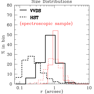
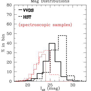
Figure 9: Left panel: size distributions for VVDS and GOODS-S galaxies. The size measure used is $r\equiv\sqrt{\pi AB}$, where $A$ and $B$ are the ellipse axes (see text). Increased seeing and noise in the ground-based observations shift the peak of the size distribution to larger sizes, and also change the shape of the distribution. Right panel: corresponding total magnitude distributions. The distribution for GOODS-S galaxies peaks about two magnitudes fainter than for the VVDS; but the spectroscopic samples have very similar magnitude and size distributions.

For different public datasets, different size measures are available. In the GOODS data, the ellipse axes, half-light radius, (filtered) isophotal area, Gaussian FWHM, and Kron aperture were all cataloged. For the VVDS data on the other hand, only the ellipse axes were available. For the HST data we found that the filtered isophotal area above the analysis threshold (SExtractor output parameter ISOAREAF_IMAGE) gave the best results for our purposes when measuring the angular area of the galaxies, giving the tightest SB($z$) relation. In Table 1, we show that the scatter of SB($z$) for the space-based data increases by a large amount for all galaxy types when we use the A_IMAGE and B_IMAGE ellipse axis parameters, instead of ISOAREAF_IMAGE, to measure the angular area.

We quantify the impact of the algorithm used to measure area in terms of the impact of a degradation in the image quality due to seeing. In Fig. 8 we apply a transformation to the galaxy sizes,

$$r^{\prime}=\sqrt{r_{0}^{2}+r_{\rm seeing}^{2}},$$ (17)

for the red galaxies ($T=[0,1,2]$) and then recompute the RMS scatter in the ${\rm SB}(z)$ relation for those galaxies. We can see that in order to make optimal use of SB information for photometric redshifts, one of the primary issues is that one needs a size measure that is precise even in the presence of noise and seeing: Fig. 8 shows that adding 1” of seeing to the isophotal area measurement increases the scatter in ${\rm SB}(z)$ by about 10%, but if the ellipse area is used for the measurement, there is about a 80% increase in scatter for the same amount of seeing.

We also see in Fig. 5 and Table 1 that the best-fit slope of the red galaxies when measured from the ground is much shallower than the best-fit slope when measured from space. Recall that we expect the blue and intermediate galaxies to have a shallow slope because they are actively evolving with $z$, but the red galaxies should have a steep slope even in the presence of seeing. However, the ground-based observations in Fig. 5 clearly have a minimum SB cutoff at ${\rm SB}\approx 26.5$ mag/arcsec², below which no sources are detected. This means that the increased scatter due to the seeing and bad size measure naturally leads to a shallower slope, because larger scatter means that the points in the SB population which would be measured below the cutoff are instead not observed, while the points that scatter to larger SB are unaffected. The net result is similar to that which would be produced by a Malmquist bias, which will also affect any flux-limited SB($z$) measurement (our sample should be largely free from the Malmquist magnitude bias itself because, as illustrated in the right panel of Fig. 9, the spectroscopic sample of galaxies which we are using is well above the flux limit of the photometric data).

Fig. 5, Table 1, and Fig. 8 together show the performance that we would need from a ground-based size measurement if we intend it to be useful for photo-z’s. For the space-based data with the isophotal size measure, the seeing starts to degrade the scatter around $r_{\rm seeing}\approx 1$”, so ideally the seeing from the ground should be less than this in order to obtain the most constraining power. Regarding the sensitivity, we note that purely for the purposes of constraining photometric redshifts, as long as the calibration sample is representative of the total sample, the photo-z measurement should be unbiased, regardless of what the SB detection threshold is. If for other purposes we want to measure the slope of SB($z$) in an unbiased way, i.e. with a slope that is not made shallower by the combination of seeing and noise, a planned survey with a similar depth ($z_{\rm med}\approx 0.7$) from the ground should be sensitive enough so that the detection threshold for galaxies is below 26.5 mag/arcsec²; this requirement will change for a deeper survey, but at the same time the SB detection threshold naturally becomes more sensitive as signal-to-noise increases.

4.2 Magnitude Prior

Figure 10: Left panel: $P(z|m)$ for three equal magnitude bins in the GOODS-N data. As the sample becomes fainter, the peak of the distribution moves slightly to higher redshift and the histogram becomes appreciably broader. Right panel: $P(z|{\rm SB})$ for three equal SB bins in the GOODS-N data. The $z$-distribution for $P(z|{\rm SB})$ doesn’t broaden as much as $P(z|m)$ does for faint samples, and the shift of the peak is more pronounced.

Another possible approach to solving the problem illustrated in Fig. 4 is to use the overall brightness of a galaxy as measured in one of the photometric bands; recall that in the template fitting procedure, in Eq. (6), only the colors and not the brightness of the galaxy are used. If we take ${\bf O}\equiv I$ (the $I$-band magnitude) in Eq. (2), then we can use this information to try to break the degeneracies. Similar techniques have been used in previous studies (see e.g. Benitez, 2000; Ilbert et al., 2006; Brodwin et al., 2006; Feldmann et al., 2006; Mobasher et al., 2007, among others). In Benitez (2000) the author demonstrates how to self-consistently compute a magnitude prior of this type from the galaxy data under study. We do not take that approach, and further make the simplifying assumption that $P(z,T|{\bf O})=P(z|m)$, i.e. galaxy type is statistically independent of magnitude. We take our prior information about the magnitude distribution of galaxies with redshift from the DEEP2 survey (Coil et al., 2004). In that survey they found the following probability density function (PDF) for their spectroscopic sample:

$$P(z|I)\propto dN/dz\propto z^{2}\exp(-z/z_{0}),$$ (18)

where $z_{0}$ is a function of the $I$-band magnitude. The parameter $z_{0}$ is fitted for in Table 3 of (Coil et al., 2004) and we extrapolate linearly to deeper redshifts from their fit. From the shape of $P(z|I)$ distribution plotted in Fig. 10, we can anticipate that the effect of applying a magnitude prior will be to always favor the lower redshift minimum in a $P(z,T)$ probability distribution. Since most galaxies really are at low redshift, we will see that this approach works well; however, using a magnitude prior exclusively would not be expected to work well if one is interested primarily in faint galaxies, since a magnitude prior does not provide much information about faint galaxies, where the prior has a long tail out to high redshift. We can see that the SB prior, plotted in the right panel, does not suffer from this effect, providing a complementary constraint for faint galaxy samples.

5 Results

In this section we will analyze the results of applying our photo-z algorithm to each of these datasets with SB priors. We will also examine the bias and scatter in our measurement errors.

5.1 Datasets

We use the Great Observatories Origins Deep Survey South (GOODS-S) and the VIMOS VLT Deep Survey (VVDS) as our calibration samples (Giavalisco et al., 2004; Vanzella et al., 2005; Le Fèvre et al., 2004b, a, 2005). The ESO CDF-S master spectroscopic catalog contains 1115 galaxies with spectroscopic redshifts, of which we use 603 that have spectroscopic redshift confidence $\geq 95$%, i.e. we select those that have quality factors greater than or equal to “B,” “3,” and “2.0” from the following sources: VLT / FORS2 spectroscopy Version 1.0; VIMOS VLT Deep Survey (VVDS) Version 1.0; and Szokoly et al. (2004). The VVDS spectroscopic catalog contains 8981 objects from the VVDS-F02 Deep field. Of these, 4180 objects meet our quality criterion ($\geq 95$% confidence in the spectroscopic redshift), corresponding to quality flags 3, 4, 9, 13, 14, and 19. We use 2090 spectra to calibrate our method on the ground based data. We then take the GOODS-N field, which contains 1814 spectra, and the other half of the VVDS data, to test our photo-z method on data which are distinct from the calibration sample. All results testing the performance of the SB and combination SB+mag priors are based on these independent calibration and test data sets.

The magnitude and size distributions of the sample of galaxies under study are shown in Fig. 9. We can see that while the spectroscopic samples are very similar, the total size and magnitude distributions of the galaxies are substantially different for the ground and space data. This is because the HST data that we evaluate have a substantially higher signal-to-noise ratio for the sizes and magnitudes. This significantly affects the measurement of SB in each sample as well as the performance of the SB and magnitude priors.

In order to evaluate the performance of the template-fitting photo-z algorithm, and any improvements that applying priors produces, we define as a figure of merit

$$\Delta=\frac{z_{p}-z_{s}}{1+z_{s}},$$ (19)

which is the fractional error in $1+z_{p}$, where $z_{p}$ is the photometric redshift estimate from Eq. (3). For a population of galaxies, $\langle\Delta\rangle$ and $\sigma_{\Delta}$ measure the photo-z bias and the RMS size of the fractional error in $1+z$.

Instead of applying a correction to the photometric zero-points and training the templates using the calibration sample, as in e.g. Ilbert et al. (2006), we adopt a simpler and largely equivalent procedure of fitting the bias (ignoring outliers) on the calibration set. First we find a polynomial fit for the bias $F(z_{s})=(z_{p}-z_{s})$ for all galaxies with $|\Delta|<0.5$ in each redshift bin in the calibration set, and then for every redshift in the test sample we apply the correction

$$z_{p}^{\prime}=z_{p}-F(z_{p}).$$ (20)

We note that a correction of this type is only expected to work well in regions adequately sampled by the spectroscopic redshift sample, while a correction to the magnitude zero-points may be effective over a larger range. The black points and histograms in Fig. 11 and Tab. 2 show the characteristics of the unweighted photo-z template fitting algorithm on the test sample after the correction has been applied.

5.2 Performance without Priors

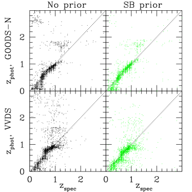
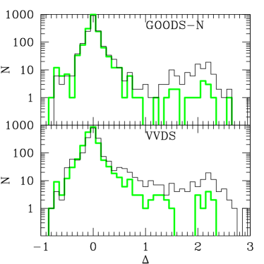
Figure 11: Left panel: Scatter plot of spectroscopic vs photometric redshift. Right panel: corresponding histogram of fractional error in $(1+z)$, $N(\Delta)$, where $\Delta\equiv(z_{p}-z_{s})/(1+z_{s})$. The green points and thicker histogram have the SB prior, while the black points/histogram have no prior applied. The lower panels contain the ground based data, 2091 galaxies from the VVDS survey, while the upper has 1814 HST galaxies from the GOODS-N field. In each case these data are separate from the calibration datasets.

The performance of the template-based photometric redshift estimator without priors on the GOODS and VVDS data sets is comparable with that found by other groups (Mobasher et al., 2007; Ilbert et al., 2006). The dispersion in the photometric redshift relation, defined at the 68^th percentile of the distribution, has a scatter of $\sigma_{68}\leq 0.08$ for redshifts $z<1.3$, and $\sigma_{68}\leq 0.14$ at redshifts $z>1.3$. If all of the data, including outliers, is considered, the dispersion of the photo-z relation is substantially larger ($>0.45$), which demonstrates the non-Gaussian nature of the photometric redshift errors, which arises due to the presence of the outliers or degenerate points (see Fig. 11). As noted by Mandelbaum et al. (2007), the small bias in the uncorrected (i.e. no correction of the form Eq. (20)) photo-z’s without priors is due to a fortuitous cancellation: the outliers which scatter to high $z$ cancel the bulk of the distribution which is biased low.

As discussed in Sec. 4, the dominant failure mode for this kind of photo-z procedure is mistaking a 4000 Å break for a Lyman break, which is visible on the scatter plots in Fig. 11 as a region in which $z_{s}\lesssim 1$ but $z_{p}\gtrsim 2$; this outlier population is composed of galaxies whose probability distribution $P(z,T)$ has multiple peaks (e.g. the galaxies in Fig. 3). Another type of failure can happen when points on both sides of the rest-frame 4000 Å break are not observed in the survey filters. We can see this in the VVDS where the performance of the unweighted algorithm suffers at redshifts at $z\gtrsim 1.2$ due to the lack of $z$-band data: at these redshifts, the VVDS outlier fraction and $\sigma_{68}$ increase sharply as the 4000 Å break redshifts out of the $I$-band; unfortunately, the $J$ and $K_{s}$ bands are much shallower than their optical counterparts and so do not help constrain high-$z$ galaxy photo-z’s. A similar phenomenon is visible in both VVDS and GOODS for galaxies with $z<0.4$, due to the lack of deep $u$-band imaging.

5.3 SB Prior Performance

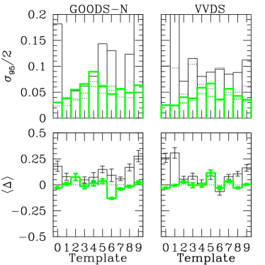
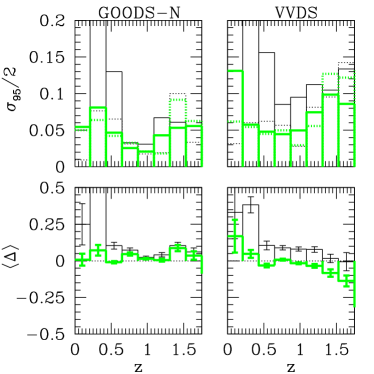
Figure 12: Left panel: bias ($\langle\Delta\rangle$) and scatter at the (solid) 95^th or (dotted) 68^th percentile as a function of template. Right panel: bias and scatter as a function of redshift. The thin black histograms have no prior applied, while the thick green histograms show the results with the SB prior. The SB prior improves both scatter and bias for essentially all templates and redshifts. The improvement at high redshift is greater for the GOODS data.

Fig. 12 shows a breakdown of the impact of the SB prior on the photo-z error distribution in different redshift and type bins; we can see that the SB prior improves bias and scatter on the independent test sample in almost all redshift and template bins. We characterize the scatter in the photometric redshifts as the dispersion given at the 95^th and 68^th percentiles of the distribution, which are denoted by solid ($\sigma_{95}/2$) and dotted ($\sigma_{68}$) lines respectively; the two measures of scatter differ in how sensitive they are to outliers. After the SB prior is applied, we obtain $\sigma_{95}/2<5$% for the GOODS-N and $\sigma_{95}/2<8$% for the VVDS data in each bin in the redshift range $0.4<z<1.3$. The largest improvement in $\sigma_{95}$ is in the low redshift bins $z<0.6$ for the GOODS and $z<1.3$ for the VVDS data, because the SB prior eliminates the largest number of outliers in these bins; we can see that outliers increase the scatter at $z<0.6$ by a factor of 2–3 for the GOODS data and by a factor of 1.5–2 for redshifts $z<1.3$ in the VVDS data. At higher redshifts the photo-z algorithm performs better on the space-based data from GOODS, due to the higher signal-to-noise, better size measurement, and $z$ band data. For the templates, the largest improvements in accuracy and precision are gained for the reddest (types 0 and 1) and bluest (types 8 and 9) galaxies. For the very old and red galaxy types, this is to be expected, because they evolve passively with redshift. As we see in Fig. 5, this means that galaxy types that have steep slopes close to $10\log{(1+z)}$ provide the strongest redshift constraints. For the very young and blue galaxies, we see from Fig. 6 that the absolute SB distribution is very tight for these types, so even though they have a shallow SB($z$) slope the prior is able to provide a constraint on their redshift.

We can gain some intuition about the physical reasons for the difference between the SB($z$) relation for the red and blue galaxy types by considering the surface brightness of a galaxy population with characteristic luminosity $L_{0}$ and size $R_{0}$:

$${\rm SB} \propto \frac{L_{0}}{R_{0}^{2}}\frac{(1+z)^{q}}{(1+z)^{2\rho}}\frac{1}{(1+z)^{4}},$$ (21)

where the exponents $q$ and $\rho$ describe the luminosity and size evolution of the sample, respectively. Studies of starbursting galaxies (Dahlen et al., 2007) have indicated that the size evolution of these galaxies is fit by $\rho\approx-1$. Willmer et al. (2006) find that $M^{*}_{B}$ for blue galaxies in the DEEP2 survey brightens by approximately 1.3 per unit redshift, i.e. $q\approx 0.5$. Therefore, ignoring selection effects, we see that for blue galaxies a combination of size and luminosity evolution should partially cancel the geometric factor of $(1+z)^{-4}$. We observe this in our data: the general trend in Fig. 5 is that for the bluer galaxies, evolution and selection together produce an effect that cancels the $(1+z)^{-4}$ evolution, while for the red galaxies, the effect is much less pronounced. This is consistent with our knowledge that red galaxies evolve much less than blue galaxies do.

We can also see how the bias $\langle\Delta\rangle$ is improved in each redshift and template bin. By eliminating the high-$z$ outliers, we achieve bias of less than 5% in each redshift bin in the range $0.4<z<1.3$ for the GOODS data, and less than 4% for the VVDS in the same range. When the SB prior is applied, the photo-z estimator continues to perform well outside this redshift range on the GOODS sample, while for the VVDS, there is larger bias at very low and very high $z$. This is due primarily to the fundamental limitations of the VVDS survey bands (no deep infrared data) we have discussed previously, as well as the issues that can affect the SB prior in ground-based observations: seeing, sensitivity, and size measurement (see Sec. 4.1.3).

Table 2 shows the global bias ($\langle\Delta\rangle$), scatter ($\sigma_{\Delta}$, $\sigma_{95}$, $\sigma_{68}$), and fraction of outliers ($N(|\Delta|>0.2)$) for the SB, magnitude, and combination priors for our GOODS and VVDS test samples. Both the magnitude and SB priors have comparable effects on the fraction of outliers in the photo-z relation, reducing it by a factor of 2 before any further cuts. If the goal of an analysis is as small a scatter as possible then applying both the magnitude and SB prior produces the best results for both GOODS and VVDS.

We also show in Table 2 a simple way to reduce the outlier fraction in the results of our photo-z algorithm. First we sort the galaxies on the value of the posterior probability $P(z,T|{\bf C},{\bf O})$, i.e. the final $\chi^{2}$, at the best-fit $(z,T)$. Then the subsequent rows after the first in each subsection of Table 2 are produced by cutting a certain fraction of the worst-fitting (highest $\chi^{2}$) galaxies from the sample and then evaluating the bias and scatter of the remainder. For the GOODS data, this produces an improvement in the scatter and outlier fraction as well as the bias; however for the VVDS, making this cut entails a tradeoff between bias and scatter. In both cases we can achieve an outlier fraction of $\leq 2$% if we are willing to sacrifice 20% of the sample.

VVDS

Prior	cut	$\langle\Delta\rangle$ $\pm$	$\frac{\sigma_{\Delta}}{\sqrt{N}}$	$\sigma_{\Delta}$	$\sigma_{68}$	$\sigma_{95}/2$	outl.
No prior	100	11.9 $\pm$	1.1	48.9	6.2	11.7	15.7
	99	11.8 $\pm$	1.1	48.7	6.2	11.6	15.7
	95	12.0 $\pm$	1.1	48.8	6.3	11.8	16.1
	80	13.5 $\pm$	1.2	50.0	6.6	12.7	17.8
Mag	100	-0.4 $\pm$	0.5	25.0	5.4	5.8	7.1
	99	-1.4 $\pm$	0.4	20.1	5.4	5.6	6.6
	95	-1.7 $\pm$	0.4	17.2	5.1	5.0	5.7
	80	-3.3 $\pm$	0.2	10.0	4.4	3.8	1.5
SB	100	-1.4 $\pm$	0.5	24.0	5.1	5.7	6.2
	99	-2.2 $\pm$	0.4	19.8	5.1	5.5	5.8
	95	-2.6 $\pm$	0.4	17.4	4.9	5.0	4.7
	80	-3.5 $\pm$	0.3	11.1	4.3	4.0	1.7
Both	100	-2.4 $\pm$	0.4	20.5	5.4	5.3	5.4
	99	-2.7 $\pm$	0.4	18.5	5.4	5.2	5.1
	95	-3.3 $\pm$	0.3	14.9	5.2	4.7	4.0
	80	-3.9 $\pm$	0.3	10.3	4.6	4.0	1.3

GOODS-N

cut	$\langle\Delta\rangle$ $\pm$	$\frac{\sigma_{\Delta}}{\sqrt{N}}$	$\sigma_{\Delta}$	$\sigma_{68}$	$\sigma_{95}/2$	outl.
100	11.8 $\pm$	1.1	48.5	4.2	9.4	11.9
99	11.0 $\pm$	1.1	46.4	4.1	8.6	11.3
95	10.0 $\pm$	1.1	44.0	4.0	7.4	10.7
80	9.8 $\pm$	1.2	43.9	4.1	7.3	10.5
100	3.2 $\pm$	0.7	27.8	3.9	4.9	7.8
99	2.1 $\pm$	0.5	23.1	3.9	4.7	7.3
95	0.8 $\pm$	0.3	14.1	3.7	4.3	6.3
80	-0.2 $\pm$	0.2	9.1	3.1	3.0	1.9
100	1.5 $\pm$	0.6	23.8	3.7	4.5	5.8
99	0.9 $\pm$	0.5	21.0	3.6	4.4	5.4
95	-0.1 $\pm$	0.3	13.1	3.4	4.0	4.4
80	-0.02 $\pm$	0.3	10.9	3.0	3.0	2.7
100	1.3 $\pm$	0.5	21.4	3.5	4.1	5.5
99	0.4 $\pm$	0.4	16.9	3.5	4.0	5.0
95	0.1 $\pm$	0.3	12.7	3.3	3.7	4.4
80	-0.3 $\pm$	0.2	9.3	2.8	2.7	2.0

Table 2: Summary of photo-z performance results for unweighted, magnitude, SB, and combination priors for VVDS (left) and GOODS-N (right). The subsequent rows for each prior beyond the first show how cutting a certain fraction of the galaxies based on the combination goodness-of-fit of the templates and prior (i.e. the final posterior $\chi^{2}$ value) enables one to trade improved scatter for slightly worse bias, eliminating a larger fraction of the outliers. The columns of the table are the fraction of sample remaining, $\langle\Delta\rangle$ and uncertainty, $\sigma_{\Delta}$, $\sigma_{\Delta}$ at the 68^th percentile, $\sigma_{\Delta}$ at the 95^th percentile, and fraction of outliers, all expressed as percentages; we follow the convention and define an outlier as having $|\Delta|>0.2$.

5.4 Applications to weak lensing

Lensing tomography refers to the use of depth information in the source galaxies to get three-dimensional information on the lensing mass (Hu, 1999). By binning source galaxies in photo-z bins, the evolution of the lensing power spectrum can be measured. This greatly improves the sensitivity of lensing to dark energy in cosmological applications. The relative shift in the amplitudes of the lensing spectra is sensitive to the properties of dark energy. It depends on both distances and the growth of structure, thus enabling tests of dark energy or modified gravity explanations for the cosmic acceleration. Any errors in the bin redshifts propagate to the inferred distances and growth factors and thus degrade the ability to discriminate cosmological models.

The capability of lensing surveys to meet their scientific goals will depend on our ability to characterize the photo-z scatter, bias and fraction of outliers. Photometric redshifts must be calibrated with an appropriate sample of spectroscopic redshifts (Huterer et al., 2006; Ma et al., 2005). This may be done more cheaply by using auto- and cross-correlations of photometric and spectroscopic redshifts samples (Schneider et al., 2006), which can also be used to estimate the redshift distribution for a galaxy sample where the calibration data is incomplete (see also Schneider et al., 2006).

For lensing power spectrum measurements, broad bins in photo-z are sufficient – bin width $\Delta z\simeq 0.2$ or larger. This makes photo-z scatter less of an issue, since wide area surveys average over million(s) of galaxies per bin. However residual bias in the estimated mean redshift per bin leads to an error in cosmological parameters; this systematic error can dominate the error budget if the photo-z’s are not well characterized and calibrated. In Huterer et al. (2006); Ma et al. (2005); Newman et al. (2006) it is shown that the next generation ground based surveys that cover $\sim 1000$ square degrees require residual bias levels below 0.01, and our method is close to this goal in the $0.4<z<1.3$ range; however the more ambitious surveys planned by LSST and SNAP require levels below 0.002. Such an exquisite control over photo-z biases requires improvements in photo-z techniques and very demanding spectroscopic calibration data.

Our results on the surface brightness prior show that it will be valuable in eliminating outliers that can bias photo-z’s. In the literature outlier clipping is often performed before photo-z’s are evaluated, but there is not a well established basis for how the clipping can be done with real data. This is part of the reason for why photo-z’s do not perform as well on data as expected from tests on simulated galaxy colors. With more realistic testing, we expect that the surface brightness prior will emerge as an essential part of photo-z measurements for lensing and other applications. Also of value is understanding the relation to galaxy type and redshift: for lensing it is permissible to use sub-samples that have well-behaved redshift distributions (see Jain et al. (2007) for an application of this idea to “color tomography”).

Lensing conserves surface brightness, but it can introduce magnification bias in the apparent magnitude. Hence using magnitude priors can cause subtle biases in lensing measurements; e.g., behind galaxy clusters magnitudes are brighter than in the field. Thus photo-z’s estimated with a magnitude prior would place galaxies that are behind clusters at lower redshift than galaxies that are in the field, and the effect would be more pronounced for more massive clusters compared to smaller ones, thus biasing cosmological inferences from lensing measurements. While the bias is expected to be small, at the percent level, it does argue in favor of surface brightness priors for precision lensing measurements.

While we have discussed weak lensing induced shear correlations, similar conclusions apply to other lensing applications such as galaxy-shear cross-correlations (known as galaxy-galaxy lensing and discussed recently by Mandelbaum et al. (2007)). For cluster lensing, i.e. making maps of the projected mass distribution using weak and strong lensing, the scatter in the photo-z relation is more important since only the source galaxies in the cluster field provide useful lensing information.

6 Discussion

We have shown that using the surface brightness-redshift relation, we can improve template-based photo-z results for both ground and space data. Our main result, presented in Sec. 5, shows how the SB prior is able to help eliminate much of the color-redshift degeneracy that is present for many galaxies in the GOODS and VVDS samples. When compared to a standard unweighted redshift estimator, SB priors reduce the fraction of outliers in the photo-z relation from 12–16% to $\sim$6%. This results in a decrease in the scatter in the photo-z relation (as defined by the 95^th percentile of the distribution) by a factor of two or more, while the bias improves from a value of $\Delta\sim 0.1$ to $\Delta\sim 0.05$; almost all redshift and type bins improve in the VVDS data, whereas the GOODS data improves likewise for all types but with an especially large effect at redshifts $z<0.6$.

At redshifts $z>1.3$ the limitations of the passbands used in the VVDS give rise to a bias that becomes more negative with increasing redshift. The utility of the SB prior is dependent on seeing and the size measures provided; in the VVDS data, the sole public size measure (ellipse area measured by SExtractor) is not precise enough to optimally measure the surface brightness-redshift relation. We expect that more sophisticated techniques, such as fitting a light profile, would reduce the sensitivity of the SB prior to seeing; in particular, we require a size estimator that minimizes the scatter in the SB($z$) relation. If a ground-based survey can precisely measure the angular area of galaxies and achieve a seeing of 1” or less, with a representative calibration sample that has the same sensitivity, then such a ground-based survey should be able to do almost as well as one from space with respect to constraining photo-z’s using the SB.

Since our current application utilizes spectroscopic data to calibrate and test the SB prior, we are necessarily restricted to studying bright galaxies. Such a regime naturally favors a magnitude prior; as Fig. 10 shows, the bright galaxy population is almost exclusively at low redshift. As the galaxies become fainter, the magnitude prior will have less and less predictive power; unfortunately, since most galaxies are faint, this is precisely the galaxy population we are most interested in obtaining photometric redshifts for. We do not expect the SB prior to suffer from this effect as much; if the sizes of galaxies are measured carefully so as to minimize the scatter in the SB($z$) relation, then the SB prior should retain its statistical power for faint galaxies as well.

Based on these results we expect, therefore, that the use of SB in constraining photometric redshifts (whether using a template based approach, neural networks, or other empirical relations) can substantially improve the robustness of the application of photo-z’s in cosmology. The details of the application and its impact will be application dependent. In some applications, such as WL tomography (Huterer et al., 2006; Ma et al., 2005), it is important for the measured redshifts to be as unbiased as possible, while others, such as Baryon Oscillations, are more sensitive to the scatter in the measurement. Subsequent papers will address the question of optimal measures for size from ground-based data and the resulting improvements in the SB prior.

References

- Abdalla et al. (2007) Abdalla F. B., Amara A., Capak P., Cypriano E. S., Lahav O., Rhodes J., 2007, arXiv:0705.1437 [astro-ph]
- Arnouts et al. (1999) Arnouts S., Cristiani S., Moscardini L., Matarrese S., Lucchin F., Fontana A., Giallongo E., 1999, MNRAS, 310, 540
- Babbedge et al. (2004) Babbedge T. S. R., et al., 2004, MNRAS, 353, 654
- Banerji et al. (2008) Banerji M., Abdalla F. B., Lahav O., Lin H., 2008, MNRAS, 386, 1219
- Benitez (2000) Benitez N., 2000, ApJ, 536, 571
- Bolzonella et al. (2000) Bolzonella M., Miralles J.-M., Pelló R., 2000, A&A, 363, 476
- Brodwin et al. (2006) Brodwin M., et al., 2006, ApJ, 651, 791
- Brodwin et al. (2006) Brodwin M., Lilly S. J., Porciani C., McCracken H. J., Le Fèvre O., Foucaud S., Crampton D., Mellier Y., 2006, ApJS, 162, 20
- Bruzual & Charlot (2003) Bruzual G., Charlot S., 2003, MNRAS, 344, 1000
- Bruzual A. & Charlot (1993) Bruzual A. G., Charlot S., 1993, ApJ, 405, 538
- Coil et al. (2004) Coil A. L., Newman J. A., Kaiser N., Davis M., Ma C.-P., Kocevski D. D., Koo D. C., 2004, ApJ, 617, 765
- Collister et al. (2007) Collister A., et al., 2007, MNRAS, 375, 68
- Connolly et al. (1995) Connolly A. J., Csabai I., Szalay A. S., Koo D. C., Kron R. G., Munn J. A., 1995, AJ, 110, 2655
- D’Abrusco et al. (2007) D’Abrusco R., Staiano A., Longo G., Brescia M., Paolillo M., De Filippis E., Tagliaferri R., 2007, ApJ, 663, 752
- Dahlen et al. (2007) Dahlen T., Mobasher B., Dickinson M., Ferguson H. C., Giavalisco M., Kretchmer C., Ravindranath S., 2007, ApJ, 654, 172
- Feldmann et al. (2006) Feldmann R., et al., 2006, MNRAS, 372, 565
- Firth et al. (2003) Firth A. E., Lahav O., Somerville R. S., 2003, MNRAS, 339, 1195
- Giavalisco et al. (2004) Giavalisco M., et al., 2004, ApJ, 600, L93
- Hu (1999) Hu W., 1999, ApJ, 522, L21
- Huterer et al. (2006) Huterer D., Takada M., Bernstein G., Jain B., 2006, MNRAS, 366, 101
- Ilbert et al. (2006) Ilbert O., et al., 2006, A&A, 457, 841
- Jain et al. (2007) Jain B., Connolly A., Takada M., 2007, JCAP, 0703, 013
- Kurtz et al. (2007) Kurtz M. J., Geller M. J., Fabricant D. G., Wyatt W. F., Dell’Antonio I. P., 2007, AJ, 134, 1360
- Le Fèvre et al. (2004a) Le Fèvre O., et al., 2004a, A&A, 428, 1043
- Le Fèvre et al. (2004b) Le Fèvre O., et al., 2004b, A&A, 417, 839
- Le Fèvre et al. (2005) Le Fèvre O., et al., 2005, A&A, 439, 845
- Li et al. (2006) Li L., Zhang Y., Zhao Y., Yang D., 2006, astro-ph/0612749
- Lubin & Sandage (2001) Lubin L. M., Sandage A., 2001, AJ, 122, 1084
- Ma et al. (2005) Ma Z.-M., Hu W., Huterer D., 2005, ApJ, 636, 21
- Madau (1995) Madau P., 1995, ApJ, 441, 18
- Mandelbaum et al. (2007) Mandelbaum R., et al., 2007, arXiv:0709.1692 [astro-ph]
- Margoniner & Wittman (2007) Margoniner V. E., Wittman D. M., 2007, arXiv:0707.2403 [astro-ph]
- Mobasher et al. (2007) Mobasher B., et al., 2007, ApJS, 172, 117
- Newman et al. (2006) Newman J., et al., 2006, in Marvel K. B., ed., Bulletin of the American Astronomical Society Vol. 38, Calibrating Photometric Redshifts for LSST. American Astronomical Society, Washington, D.C., pp 1018–+
- Oyaizu et al. (2008) Oyaizu H., Lima M., Cunha C. E., Lin H., Frieman J., Sheldon E. S., 2008, ApJ, 674, 768
- Schneider et al. (2006) Schneider M., Knox L., Zhan H., Connolly A., 2006, ApJ, 651, 14
- Szokoly et al. (2004) Szokoly G. P., et al., 2004, ApJS, 155, 271
- Tolman (1930) Tolman R. C., 1930, Proceedings of the National Academy of Science, 16, 511
- Tolman (1934) Tolman R. C., 1934, Relativity, Thermodynamics, and Cosmology. Relativity, Thermodynamics, and Cosmology, Oxford: Clarendon Press, 1934
- Vanzella et al. (2004) Vanzella E., et al., 2004, A&A, 423, 761
- Vanzella et al. (2005) Vanzella E., et al., 2005, A&A, 434, 53
- Willmer et al. (2006) Willmer C. N. A., et al., 2006, Astrophys. J., 647, 853
- Wittman et al. (2007) Wittman D., Riechers P., Margoniner V. E., 2007, ApJ, 671, L109
- Wray & Gunn (2008) Wray J. J., Gunn J. E., 2008, Astrophys. J., 678, 144