On the nature of outflows in intermediate-mass protostars: a case study of IRAS 20050+2720

Abstract

Context. This is the third of a series of papers devoted to study in detail and with high-angular resolution intermediate-mass molecular outflows and their powering sources.

Aims. The aim of this paper is to study the intermediate-mass YSO IRAS 20050+2720 and its molecular outflow, and put the results of this and the previous studied sources in the context of intermediate-mass star formation.

Methods. We carried out VLA observations of the 7 mm continuum emission, and OVRO observations of the 2.7 mm continuum emission, CO ($J$=1$\rightarrow$0), C¹⁸O ($J$=1$\rightarrow$0), and HC₃N ($J$=12$\rightarrow$11) to map the core towards IRAS 20050+2720. The high-angular resolution of the observations allowed us to derive the properties of the dust emission, the molecular outflow, and the dense protostellar envelope. By adding this source to the sample of intermediate-mass protostars with outflows, we compare their properties and evolution with those of lower mass counterparts.

Results. The 2.7 mm continuum emission has been resolved into three sources, labeled OVRO 1, OVRO 2, and OVRO 3. Two of them, OVRO 1 and OVRO 2, have also been detected at 7 mm. OVRO 3, which is located close to the C¹⁸O emission peak, could be associated with IRAS 20050+2720. The mass of the sources, estimated from the dust continuum emission, is 6.5 $M_{\odot}$ for OVRO 1, 1.8 $M_{\odot}$ for OVRO 2, and 1.3 $M_{\odot}$ for OVRO 3. The CO ($J$=1$\rightarrow$0) emission traces two bipolar outflows within the OVRO field of view, a roughly east-west bipolar outflow, labeled A, driven by the intermediate-mass source OVRO 1, and a northeast-southwest bipolar outflow, labeled B, probably powered by a YSO engulfed in the circumstellar envelope surrounding OVRO 1.

Conclusions. The multiplicity of sources observed towards IRAS 20050+2720 appears to be typical of intermediate-mass protostars, which form in dense clustered environments. In some cases, as for example IRAS 20050+2720, intermediate-mass protostars would start forming after a first generation of low-mass stars has completed their main accretion phase. Regarding the properties of intermediate-mass protostars and their outflows, they are not significantly different from those of low-mass stars. Although intermediate-mass outflows are intrinsically more energetic than those driven by low-mass YSOs, when observed with high-angular resolution they do not show intrinsically more complex morphologies. Intermediate-mass protostars do not form a homogeneous group. Some objects are likely in an earlier evolutionary stage as suggested by the infrared emission and the outflow properties.

1 Introduction

Molecular outflow is an ubiquitous phenomenon during the earliest stages of the formation of stars of all masses and luminosities. During the last decades, many efforts have been devoted to the study and description of the physical properties of embedded low-mass protostars and their molecular outflows (e.g., Bachiller bachiller96 (1996); Richer et al. richer00 (2000)). In recent years, high-mass molecular outflows have also been studied in detail, and many surveys have been carried out towards massive star-forming regions to achieve a more accurate picture of their morphology and properties (e.g., Shepherd & Churchwell 1996a , 1996b ; Zhang et al. zhang01 (2001); Shepherd shepherd05 (2005)). In recent years, there has been a growing interest for the Young Stellar Objects (YSOs) located at the lower and the higher end of the stellar mass spectrum. Less attention has been paid to intermediate-mass protostars, with masses in the range $2\leavevmode\nobreak\ M_{\odot}\leq M_{\star}\leq 10\leavevmode\nobreak\ M_{\odot}$, which can power energetic molecular outflows. In fact, only few deeply embedded intermediate-mass protostars are known to date, and only a very limited number of their outflows have been studied at high-angular resolution.

Table 1: Parameters of the observations

			Synthesized beam
		Frequency	HPBW	PA	Spectral resolution	rms noisea
Observation	Telescope	(GHz)	(arcsec)	(deg)	(km s-1)	(mJy beam-1)
2.7 mm continuum	OVRO	111.02	$7.0\times 6.4$	$-49$	$-$	1.5
CO ($J$=1$\rightarrow$0)	OVRO	115.27	$6.8\times 4.1$	$-59$	0.65	55
C18O ($J$=1$\rightarrow$0)	OVRO	109.78	$8.1\times 6.0$	$-43$	0.68	40
HC3N ($J$=12$\rightarrow$11)	OVRO	109.17	$8.1\times 6.0$	$-47$	0.69	40
7 mm continuum	VLA	143.34	$4.9\times 3.8$	$-9$	$-$	0.16

(a) For the molecular line observations the 1 $\sigma$ noise is per channel.

In order to study in detail intermediate-mass protostars and the outflows that they are powering and to compare their morphology and evolution with those of low-mass stars, we have started a project to carry out interferometric observations of dust and gas towards intermediate-mass star forming regions. The first two regions observed were IRAS 21391+5802 (Beltrán et al. beltran02 (2002); hereafter Paper I) and L1206 (Beltrán et al. 2006b ; hereafter Paper II). In this third paper, we present a thorough interferometric study of the intermediate-mass protostar IRAS 20050+2720 and of its molecular outflow. IRAS 20050+2720 is a $280\leavevmode\nobreak\ L_{\odot}$ (Froebrich froebrich05 (2005)) YSO located in the Cygnus rift at a distance of 700 pc (Dame & Thaddeus dame85 (1985)).Distances in the Cygnus region are highly uncertain for stellar objects located at Galactic longitudes close to 90°, as the kinematic distances are not reliable (e.g. Schneider et al. schneider06 (2006)). However, IRAS 20050+2720 has a Galactic longitude of $\sim$66°, being located in a region where the Cygnus rift can be distinguished from the Cygnus X complex. Therefore, the kinematic distance determined by Dame & Thaddeus (dame85 (1985)) from CO line emission is quite reliable. IRAS 20050+2720 is surrounded by a cluster of infrared stars (Chen et al. chen97 (1997)). Bachiller et al. (bachiller95 (1995)) mapped a high-velocity multipolar CO outflow in the region, previously detected by Wilking et al. (wilking89 (1989)). IRAS 20050+2720 is deeply embedded in a core that has been observed in the continuum at millimeter (Wilking et al. wilking89 (1989); Chen et al. chen97 (1997); Choi et al. choi99 (1999); Chini et al. chini01 (2001); Furuya et al. furuya05 (2005); Beltrán et al. 2006a ) and centimeter (Wilking et al. wilking89 (1989); Anglada et al. 1998a ) wavelengths, and also in different high-density tracers, such as HCO⁺ and HCN (Choi et al. choi99 (1999)), NH₃ (Molinari et al. molinari96 (1996)), CS and N₂H⁺ (Bachiller et al. bachiller95 (1995); Williams & Myers williams99 (1999)), and ¹³CO and C¹⁸O (Ridge et al. ridge03 (2003)). The source has been classified as an intermediate-mass Class 0/I protostar (Gregersen et al. gregersen97 (1997); Chini et al. chini01 (2001); Froebrich froebrich05 (2005)).

As shown by these previous studies, intermediate-mass outflows appear more collimated and less complex than previously thought (e.g. Fuente et al. fuente01 (2001)) when observed with high-angular resolution. This argues for the need of high-angular observations to better understand intermediate-mass protostars and their outflows. To accomplish the ultimate goal of our research project, which is to study and compare the properties and evolution of intermediate-mass protostars with those of their lower mass counterparts, in this last paper of the series, we put the results on the three intermediate-mass protostars studied in the context of intermediate-mass star formation. To do this, we have compiled information on outflow properties that have been derived from interferometric observations to better compare them with the ones derived for the sources in our study.

2 Observations

2.1 OVRO observations

Millimeter interferometric observations of IRAS 20050+2720 at 2.7 mm were carried out with the Owens Valley Radio Observatory (OVRO) Millimeter Array of six 10.4 m telescopes in the L (Low) and C (Compact) configurations, on April 30 and May 30, 2003, respectively. The data taken in both array configurations were combined, resulting in baselines ranging from 5.6 to 42.6 $k\lambda$, which provided sensitivity to spatial structures from about 4$\aas@@fstack{\prime\prime}$8 to 37^′′. The digital correlator was configured to simultaneously observe the continuum emission and some molecular lines. Details of the observations are given in Table 1. The phase center was located at $\alpha$(J2000) = $20^{\rm h}07^{\rm h}5\aas@@fstack{s}80$, $\delta$(J2000) = $+27\degr 28^{\prime}58\aas@@fstack{\prime\prime}1$. Bandpass calibration was achieved by observing the quasars 3C84, 3C273, and 3C345. Amplitude and phase were calibrated by observations of the nearby quasar J2015+71, whose flux density was determined relative to Uranus. The uncertainty in the amplitude calibration is estimated to be $\sim$$20\%$. The OVRO primary beam is $\sim$$64^{\prime\prime}$ (FWHM) at 115.27 GHz. The data were calibrated using the MMA package developed for OVRO (Scoville et al. scoville93 (1993)). Reduction and analysis of the data were carried out using standard procedures in the MIRIAD, AIPS, and GILDAS software packages. We subtracted the continuum from the line emission directly in the (u, v) domain for C¹⁸O ($J$=1$\rightarrow$0) and HC₃N ($J$=12$\rightarrow$11), and in the image domain for CO ($J$=1$\rightarrow$0).

2.2 VLA observations

The interferometric observations at 7 mm were carried out on January 5, 2002 using the Very Large Array (VLA) of the National Radio Astronomy Observatory (NRAO) in the D configuration. The baselines ranged from 5.4 to 140 $k\lambda$, which provided sensitivity to spatial structures from about 1$\aas@@fstack{\prime\prime}$5 to 37^′′. The phase center was set to the position $\alpha$(J2000) = $20^{\rm h}07^{\rm h}5\aas@@fstack{s}91$, $\delta$(J2000) = $+27\degr 28^{\prime}58\aas@@fstack{\prime\prime}2$. Absolute flux calibration was achieved by observing 3C286, with an adopted flux density of 1.45 Jy. Amplitude and phase were calibrated by observing 2023+318, which has a bootstrapped flux of $0.48\pm 0.01$ Jy. CLEANed maps were made using the task IMAGR of the AIPS software of the NRAO, with the ROBUST parameter of Briggs (briggs95 (1995)) set equal to 5, which is close to natural weighting. We used a Gaussian taper in the (u, v) domain when making the maps in order to enhance the extended emission in the region. The resulting synthesized beam is $4\aas@@fstack{\prime\prime}9\times 3\aas@@fstack{\prime\prime}8$ at PA =$-9\degr$, and the rms noise is 0.16 mJy beam^-1.

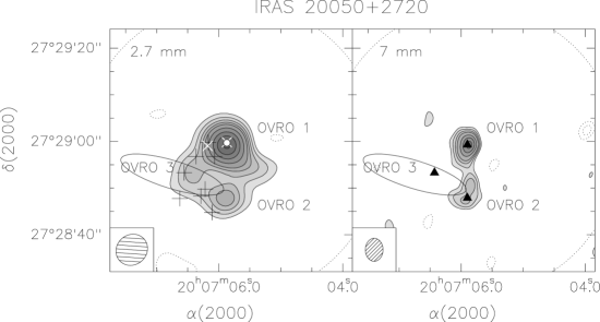
Figure 1: Map of the OVRO 2.7 mm (left panel) and the VLA 7 mm (right panel) continuum emission towards IRAS 20050+2720. The rms noise of the map, $\sigma$, is 1.5 mJy beam^-1 (left panel) and 0.16 mJy beam^-1 (right panel). The contour levels are $-5$, $-3$, 3, 5, 7, 9, 11, 15, 20, 25, and 30 times $\sigma$ (left panel), and $-4$, $-3$, 3, 4, 5, 6, 8, 10, and 12 times $\sigma$ (right panel). The synthesized beams are drawn in the bottom left corner. The error ellipse of IRAS 20050+2720 is indicated in black. The dotted circles represent the OVRO (left panel) and VLA (right panel) primary beam (50% attenuation level). Black crosses indicate the corrected position (see Sect. 3.1) of the NIR sources detected by Chen et al. (chen97 (1997)), and white crosses the position of the 3 mm sources detected by Furuya et al. (furuya05 (2005)). The white circle marks the position of the 3.6 cm VLA source reported by Anglada et al. (1998a ). Black triangles in right panel mark the OVRO 2.7 mm continuum position of the sources.

Table 2: Positions, millimeter flux densities, sizes, and masses of the cores detected towards IRAS 20050+2720

Positiona

$\lambda=2.7$mm

$\lambda=7$mm

$\alpha({\rm J2000})$

$\delta({\rm J2000})$

$I^{\rm peak}_{\nu}$ b

$S_{\nu}$ b

$I^{\rm peak}_{\nu}$ ${}^{\leavevmode\nobreak\ b}$

$S_{\nu}$ b

$\theta^{c}$

Massd

$n({\rm H_{2}})^{e}$

$N({\rm H_{2}})^{e}$

Core

20h 07m

+27° 28′

(mJy beam-1)

(mJy)

(mJy beam-1)

(mJy)

(arcsec)

($M_{\odot}$)

($10^{6}$ cm-3)

(1023 cm-2)

OVRO 1

$05\aas@@fstack{s}90$

$59\aas@@fstack{\prime\prime}3$

$\phantom{2}46.4\pm 9.3$

$\phantom{11.}65\pm 13\phantom{.1}$

$2.04\pm 0.17$

$2.88\pm 0.17$

3.3

6.5

1.3

1.4

OVRO 2

$05\aas@@fstack{s}90$

$47\aas@@fstack{\prime\prime}9$

$\phantom{1}17.1\pm 3.4$

$\phantom{1}18.0\pm 3.6\phantom{0}$

$0.97\pm 0.17$

$1.84\pm 0.17$

2.3

$1.8$

1.7

1.1

OVRO 3

$06\aas@@fstack{s}43$

$53\aas@@fstack{\prime\prime}3$

$\phantom{1}12.9\pm 2.6$

$12.9\pm 2.6$

$<0.48^{f}$

$\ldots$

$<6.7^{g}\phantom{1}$

$\phantom{.}1.3^{h}$

$\phantom{.}3.0^{h}$

$\phantom{.}1.4^{h}$

(a) Position of the 2.7 mm emission peak.
(b) Corrected for primary beam response.
(c) Deconvolved geometrical mean of the major and minor axes of the half-peak intensity contour.
(d) Circumstellar mass estimated taking into account all the emission inside the 3 $\sigma$ level, and assuming a dust temperature of 34 K (see Sect. 4.1).
(e) Average H₂ volume and column density estimated assuming spherical symmetry and a $10\%$ Helium abundance. The densities have been computed taking into account the total circumstellar mass and the size of the source at a 3$\leavevmode\nobreak\ \sigma$ emission level.
(f) 3 $\sigma$ upper limit.
(g) Source not resolved.
(h) Estimated from the peak intensity.

3 Results

3.1 Dust emission

The maps of the millimeter continuum emission around the embedded source IRAS 20050+2720  at 2.7 and 7 mm are shown in Fig. 1. The continuum emission at 2.7 mm has been resolved into three different sources, labeled OVRO 1, OVRO 2, and OVRO 3. OVRO 1 and OVRO 2 have also been detected at 7 mm, but not OVRO 3, for which an upper limit (3 $\sigma$) of 0.48 mJy beam^-1 has been estimated. OVRO 3 is not so well defined at 2.7 mm as the other two sources. However, the source is located within $\sim$$1\aas@@fstack{\prime\prime}6$ of the near-infrared (NIR) source 5 of Chen et al. (chen97 (1997); see discussion below about the correction to the positions given by these authors). The source is probably associated with IRAS 20050+2720 (Fig. 1), at least at 12 and 25 $\mu$m wavelengths. However, one cannot discard the possibility that part of the emission detected at longer wavelengths (60 and 100 $\mu$m) is associated with OVRO 1 and/or OVRO 2 as suggested by the IRAS high-resolution processed (HIRES) images. OVRO 3 is also associated with a C¹⁸O peak (see Sect. 3.3). All this lead us to consider the bump visible at 2.7 mm emission as an independent source, that we called OVRO 3. OVRO 1 and OVRO 2 are separated $\sim$$11\arcsec$ ($\sim$8000 AU at the distance of the region), while OVRO 3 is separated $\sim$$9\arcsec$ ($\sim$6000 AU) from the other two sources. The position, the flux density at 2.7 mm, the deconvolved size of the sources (measured as the geometrical mean of the major and minor axis of the half-peak intensity contour around each source), the mass, and the average volume and column density are given in Table 2.

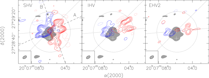
Figure 2: CO ($J$=1$\rightarrow$0) emission integrated in different velocity intervals, ($-7$, +$1$) km s^-1  for the SHV blueshifted emission (left panel; blue contours), ($11$, $19$) km s^-1 for the redshifted one (left panel; red contours), ($-14$, $-7$) km s^-1 for the IHV blueshifted emission (middle panel; blue contours), and (+$19$, +$26$) km s^-1  for the redshifted one (middle panel; red contours), ($-19$, $-14$) km s^-1 for the EHV2 blueshifted emission (right panel; blue contours), and (+$26$, +$31$) km s^-1  for the redshifted one (right panel; red contours), overlaid on the 2.7 mm continuum emission at a 3 $\sigma$ level (greyscale). Contour levels are $-5$, $-3$, 3, 5, 7, 10, 15, 20, 30 and 40 times $\sigma$, where 1 $\sigma$ is 0.6 Jy beam^-1 km s^-1 for the SHV interval, 0.5 Jy beam^-1 km s^-1 for IHV, and 0.25 Jy beam^-1 km s^-1 for EHV2. The white crosses mark the millimeter continuum positions of OVRO 1, OVRO 2 and OVRO 3. The black dashed lines in left panel outline the direction of outflows A, and B (see Sect. 3.2). The black dotted lines outline the edges of outflow A powered by OVRO 1. The synthesized beam is drawn in the bottom left corner. The dotted circle represents the OVRO primary beam (50% attenuation level).

The strongest millimeter source is OVRO 1. This source is located at the center of one of the two CO molecular outflows detected in the region (see the next section and Fig. 2), which suggests that OVRO 1 is its driving source. OVRO 1 has a core-halo structure at millimeter wavelengths, with a core that has a deconvolved diameter of $\sim$$3\aas@@fstack{\prime\prime}3$ ($\sim$2300 AU) at the half-peak intensity contour of the dust emission, and an extended and quite spherical halo or envelope that has a size of $\sim$$11\aas@@fstack{\prime\prime}3$ ($\sim$8000 AU) at the 3 $\sigma$ contour level. The source OVRO 2 has a deconvolved diameter of $\sim$$2\aas@@fstack{\prime\prime}3$ ($\sim$1600 AU) at the half-peak intensity contour of the dust emission. On the other hand, OVRO 3 is not resolved with the angular resolution of the 2.7 mm observations. These sizes are consistent with the values found for envelopes around low- and intermediate-mass protostars (e.g., Hogerheijde et al hogerheijde97 (1997), hogerheijde99 (1999); Looney et al. looney00 (2000); Fuente et al. fuente01 (2001); Paper I, Paper II). As can be seen in Fig. 1, there is extended emission surrounding the three sources, which is clearly visible at 2.7 mm but not at 7 mm. The estimated upper limit (3 $\sigma$) for the extended emission at 7 mm is 0.48 mJy beam^-1. This extended component has a size of $\sim$$19^{\prime\prime}$ ($\sim$13000 AU).

The position of the eight NIR sources detected by Chen et al. (chen97 (1997)) are indicated as black crosses in Fig. 1. We compared these positions with those of the 2MASS catalog and found that the positions reported by Chen et al. (chen97 (1997)) were systematically offset on average by $\sim$$-0\aas@@fstack{s}29$ in right ascension, and $\sim$$1\aas@@fstack{\prime\prime}4$ in declination. Therefore, before plotting them, we corrected the positions. As already mentioned, the only NIR source possibly associated with the millimeter sources detected with OVRO at 2.7 mm is source 5, whose position nearly coincides with OVRO 3. Chen et al. (chen97 (1997)) also detect a compact source at 2.7 mm with the Berkeley-Illinois-Maryland Association (BIMA) array coincident with OVRO 1. These authors estimate a flux density of $30\pm 3.5$ mJy, which is half of that derived with OVRO (see Table 2). Although Chen et al. (chen97 (1997)) locate the millimeter continuum source close to the NIR sources 6, 7, and 8, this is not the case after correcting the infrared positions. Therefore, this suggests that OVRO 1 and OVRO 2 could be deeply embedded sources still undetected at NIR wavelengths. The situation could be different for OVRO 3 because of its possible association with IRAS 20050+2720 and NIR source 5.

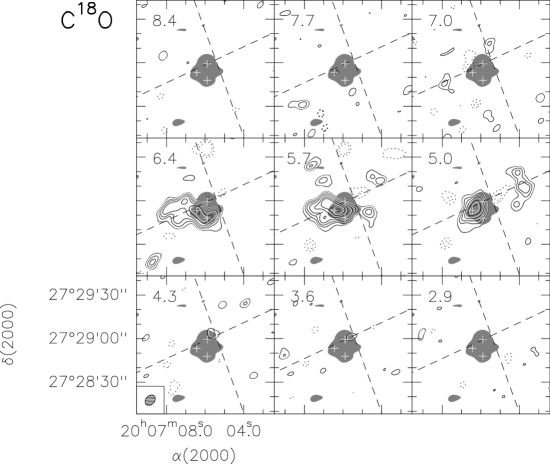
Figure 3: Velocity channel maps of the C¹⁸O ($J$=1$\rightarrow$0) emission (contours) overlaid on the 2.7 mm continuum emission at a 3 $\sigma$ level (greyscale). The systemic velocity of IRAS 20050+2720 is $6$ km s^-1. The central velocity of each channel is indicated at the upper left corner of the panels. The 1 $\sigma$ noise in one channel is 40 mJy beam^-1. Contour levels are $-5$, $-3$, 3, 5, 7, 10, 15, 20, and 30 times $\sigma$. The conversion factor from Jy beam^-1 to K is 2.10. The synthesized beam is drawn in the bottom left corner of the bottom left panel. The white crosses mark the millimeter continuum positions of OVRO 1, OVRO 2, and OVRO 3. The dashed lines outline the direction of the CO outflows A and B detected in the region (see Fig. 2).

The region has also been observed at centimeter wavelengths with the VLA by Anglada et al. (1998a ). As can be seen in Fig. 1, the source OVRO 1 coincides within $0\aas@@fstack{\prime\prime}5$ with a 3.6 cm source, with two components separated by $\sim 0\aas@@fstack{\prime\prime}3$ (Anglada et al. 1998a ).

The position of the millimeter source detected by Furuya et al. (furuya05 (2005)) with the OVRO interferometer at 3 mm is indicated as a white cross in Fig. 1. The source is clearly coincident with OVRO 1. These authors also find millimeter emission eastward of OVRO 1, which could be associated with one of the NIR sources. This suggests that another YSO could be embedded in the core (Furuya et al. furuya05 (2005)). The position of this possible embedded YSO detected by Furuya et al. (furuya05 (2005)) is also marked in Fig. 1 with a white cross. Our observations do not have enough resolution to separate this eastern emission from that of OVRO 1 and its extended envelope. The total integrated flux density measured by Furuya et al. (furuya05 (2005)) at 3 mm is 25.6 mJy. If we assume a dust absorption coefficient proportional to $\nu^{2}$, the expected flux at 2.7 mm would be $\sim 39$ mJy, which is about half of the integrated flux density measured for OVRO 1 at 2.7 mm. This is probably due to the fact that the Furuya et al. observations were carried out with more extended OVRO configurations (E and H), and thus, being somewhat less sensitive to extended emission. As a consequence of this, it is possible that part of the extended emission surrounding OVRO 1 was filtered out by the interferometer, consistent with the negative contours visible in Fig. 1 of Furuya et al. (furuya05 (2005)).

Choi et al. (choi99 (1999)) observed the region with BIMA at 3.4 mm, with a synthesized beam slightly larger than that of our 2.7 mm OVRO observations, and resolve the continuum emission into four sources, labeled A, B, C, and D. The peak position of source A is in agreement with that of OVRO 1. This source is extended and elongated towards the south and the southeast, and its structure resembles that of the extended emission surrounding OVRO 1, 2, and 3 as mapped by us at 2.7 mm.

Chini et al. (chini01 (2001)) observed the region with the single dish James Clerk Maxwell Telescope (JCMT) at 0.45, 0.85, and 1.3 mm with angular resolutions ranging from $\sim$8 to 15^′′ and detected three sources in the region, IRAS 20050+2720 MMS 1, MMS 2, and MMS 3, together with an extension to the south of MMS 1. The source IRAS 20050+2720 MMS 1 is associated with OVRO 1, 2 and 3. Beltrán et al. (2006a ) detect a similar emission with the Swedish-ESO Submillimetre Telescope (SEST) at 1.3 mm. The clump number 1 is the one associated with OVRO 1, 2, and 3. However, this clump, which has a size of $58\aas@@fstack{\prime\prime}2$, is much larger than the extended 2.7 mm emission or MMS 1, as it includes the extended southern emission as well.

Table 3: C¹⁸O ($J$=1$\rightarrow$0), and HC₃N ($J$=12$\rightarrow$11) line and physical parameters towards OVRO 1, OVRO 2 and OVRO 3 in IRAS 20050+2720

		$V_{\rm LSR}$	$\Delta V$	$T_{\rm B}$	$\int{T_{\rm B}\,{\rm d}V}$	$\theta^{a}$	$M_{\rm vir}^{b}$
Position	Molecule	(km s-1)	(km s-1)	(K)	(K km s-1)	(arcsec)	($M_{\odot}$)
OVRO 1	C18O	$4.68\pm 0.04$	$1.50\pm 0.21$	$0.94\pm 0.11$	$1.50\pm 0.07$
	HC3N	$4.82\pm 0.02$	$1.44\pm 0.05$	$3.80\pm 0.12$	$5.84\pm 0.18$	$9\aas@@fstack{\prime\prime}6$	4.3–5.7
OVRO 2	C18O	$6.33\pm 0.04$	$1.70\pm 0.10$	$1.56\pm 0.19$	$2.83\pm 0.12$	$7\aas@@fstack{\prime\prime}0^{c}$	$<$4.3–5.82
	HC3N	$5.86\pm 0.08$	$1.60\pm 0.20$	$0.85\pm 0.13$	$1.44\pm 0.17$
OVRO 3	C18O	$5.61\pm 0.03$	$1.92\pm 0.06$	$2.51\pm 0.17$	$5.14\pm 0.15$	$14$	11–15
	HC3N	$5.41\pm 0.03$	$1.30\pm 0.10$	$2.06\pm 0.14$	$2.85\pm 0.14$

(a) Deconvolved geometrical mean of the major and minor axes of the half-peak intensity contour.
(b) Estimated from Eq. 5 of Paper II for typical density distributions with $p=2.0$–1.5.
(c) Emission not resolved. Beam size.

3.2 The molecular outflow: CO emission

The CO emission towards IRAS 20050+2720 has been previously studied through lower angular resolution observations by Bachiller et al. (bachiller95 (1995)). These authors discover three bipolar molecular outflows in the region: an extremely high velocity highly collimated outflow oriented nearly east-west (labeled A in Fig. 3 of Bachiller et al.); a bipolar outflow of intermediate high velocity oriented in the northeast-southwest direction (labeled B); and a standard high velocity bipolar outflow detected along the northwest-southeast direction (labeled C). The observations reported in the present study significantly improve the angular resolution of previous outflow maps, revealing the structure of the molecular outflows in detail, as the interferometer filters out most of the extended CO emission seen in the Bachiller et al. (bachiller95 (1995)) low and intermediate velocity maps.

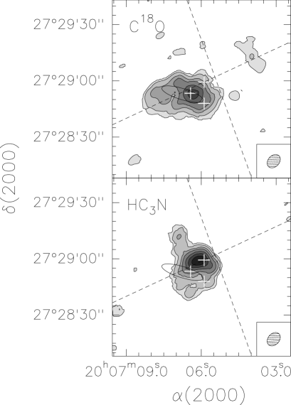
Figure 4: Integrated intensity map of the C¹⁸O ($J$=1$\rightarrow$0) (top) and the HC₃N ($J$=12$\rightarrow$11) (bottom) emission over the velocity interval (3,8) km s^-1 towards IRAS 20050+2720. Contour levels are 0.17, 0.34, 0.68, 1.0, 1.5, 2.0, and 2.5 Jy beam^-1 km s^-1 for both panels. The white crosses show the millimeter continuum positions of OVRO 1, OVRO 2, and OVRO 3. The dashed lines indicate the direction of the CO outflows A and B. The error ellipse of IRAS 20050+2720 is indicated in black. The synthesized beam is drawn in the bottom right corner of each panel.

Figure 2 shows the maps of the integrated CO ($J$=1$\rightarrow$0) emission in three different blueshifted and redshifted velocity intervals. For the sake of comparison, we chose the same velocity intervals as Bachiller et al. (bachiller95 (1995)): a standard-high velocities (SHV) interval, with ($-7$, +$1$) km s^-1 for blueshifted emission and ($11$, $19$) km s^-1 for the redshifted one; an intermediate-high velocities (IHV) interval, with ($-14$, $-7$) km s^-1 for the blueshifted emission and (+$19$, +$26$) km s^-1  for the redshifted one; and an extremely-high velocities (EHV2) interval, with ($-19$, $-14$) km s^-1 for the blueshifted emission and (+$26$, +$31$) km s^-1  for the redshifted one. The other extremely high-velocities interval, EHV1, observed by Bachiller et al. (bachiller95 (1995)) has not been mapped because our OVRO observations did not cover that range of velocities. The systemic velocity, $V_{\rm LSR}$, is roughly 6 km s^-1. As can be seen in this figure, the CO emission traces two bipolar outflows in the region, a roughly east-west outflow, coincident with outflow A of Bachiller et al. (bachiller95 (1995)), and a northeast-southwest outflow, coincident with outflow B. The outflow labeled C by Bachiller et al. (bachiller95 (1995)) and mapped at the lowest velocity interval (SHV) has not been detected. As can be seen in Fig. 3 of Bachiller et al. (bachiller95 (1995)), the outflow C, which has a PA of about $-35\degr$, has very extended lobes, especially for the blueshifted emission that reaches distances of $>$$100^{\prime\prime}$ from the IRAS source. Most of the emission of this outflow lies outside of the OVRO primary beam and, therefore, these interferometric observations are not sensitive to it. Note that one cannot rule out the possibility that part of the central emission of the outflow C overlaps that of the outflows A and B, and as it is not possible to distinguish any possible emission of the outflow C from that of the outflows A and B, we considered the outflow C as not detected in this study.

3.3 C¹⁸O emission

Figure 3 shows the velocity channel maps for the C¹⁸O ($J$=1$\rightarrow$0) emission around the systemic velocity, $V_{\rm LSR}\simeq 6$ km s^-1, overlaid on the continuum emission. The emission integrated over the central channels, velocity interval (3, 8) km s^-1, is shown in the top panel of Fig. 4. The emission is elongated in the east-west direction and peaks towards OVRO 3. C¹⁸O shows a more extended emission than the dust. In particular, it shows an elongation in the direction of the molecular outflow A, which suggests some interaction between the outflow and the envelope. The spectra taken at the position of the continuum peak of OVRO 1, OVRO 2, and OVRO 3 are shown in Figure 5. Table 3 lists the fitted parameters for C¹⁸O ($J$=1$\rightarrow$0) and HC₃N ($J$=12$\rightarrow$11). The corresponding Gaussian fits are shown in Fig. 5. As can be seen in the channel maps and the spectra, the C¹⁸O emission is associated with the three millimeter sources, with the emission towards OVRO 1 weaker than towards OVRO 2 and 3. The velocity integrated flux density of the central emission is $\sim$16 Jy km s^-1 and has a deconvolved size, measured as the geometrical mean of the major and minor axes of the half-peak intensity contour of the gas, of $\sim$$14^{\prime\prime}$ or $\sim$9800 AU.

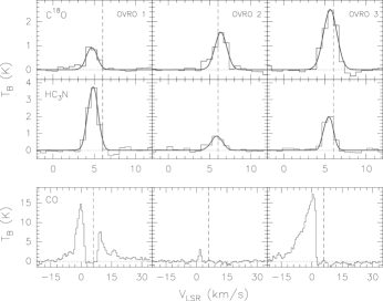
Figure 5: C¹⁸O ($J$=1$\rightarrow$0) (top), HC₃N ($J$=12$\rightarrow$11) (middle), and CO ($J$=1$\rightarrow$0) (bottom) spectra obtained at the position of OVRO 1, OVRO 2, and OVRO 3 in IRAS 20050+2720. The continuum has been subtracted. The conversion factor is 2.10 K/Jy beam^-1 for C¹⁸O, 2.14 K/Jy beam^-1 for HC₃N, and 3.30 K/Jy beam^-1 for CO. The thick grey profiles in top and middle panels are the Gaussian fits to the spectra. The dashed vertical line indicates the systemic velocity of 6 km s^-1.

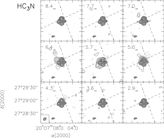
Figure 6: Velocity channel maps of the HC₃N ($J$=12$\rightarrow$11) emission (contours) overlaid on the 2.7 mm continuum emission at a 3 $\sigma$ level (greyscale). The systemic velocity of IRAS 20050+2720 is $6$ km s^-1. The central velocity of each channel is indicated at the upper left corner of the panels. The 1 $\sigma$ noise in one channel is 40 mJy beam^-1. Contour levels are $-5$, $-3$, 3, 5, 7, 10, 15, 20, 30 and 45 times $\sigma$. The conversion factor from Jy beam^-1 to K is 2.14. The synthesized beam is drawn in the bottom left corner of the bottom left panel. The white crosses mark the millimeter continuum positions of OVRO 1, OVRO 2, and OVRO 3. The dashed lines outline the direction of the CO outflows A nd B (see Fig. 2).

3.4 HC₃N emission

Figure 6 shows the velocity channel maps for the HC₃N ($J$=12$\rightarrow$11) emission towards IRAS 20050+2720, around the systemic velocity, $V_{\rm LSR}\simeq 6$ km s^-1, overlaid on the continuum emission. The emission integrated over the velocity interval (3, 8) km s^-1 is shown in the bottom panel of Fig. 4. HC₃N shows a spatial distribution different from that of C¹⁸O and the dust. This is probably because the different molecular tracers and the dust are tracing material at slightly different physical conditions. The C¹⁸O elongation along outflow A is not traced by HC₃N, which could indicate that the gas is not dense enough to excite the HC₃N ($J$=12$\rightarrow$11) transition. The spectra taken at the position of the continuum peak of OVRO 1, OVRO 2, and OVRO 3 are shown in Figure 5. The emission peaks about $4\aas@@fstack{\prime\prime}2$ east of the continuum peak position of OVRO 1, and it is clearly associated with this source. HC₃N emission is also associated with the other two sources in the region, with the emission towards OVRO 2 weaker than towards OVRO 1 and 3. Although the emission is quite compact, it shows a tail towards the northeast, and it is slightly elongated towards the southeast, along the direction of the molecular outflow A. The HC₃N emission has a velocity integrated flux density of $\sim$12.7 Jy km s^-1 and a deconvolved size of $9\aas@@fstack{\prime\prime}6$ or $\sim 6700$ AU.

4 Analysis and discussion of IRAS 20050+2720

4.1 Mass and density estimates from dust emission

Assuming that the dust emission is optically thin, we estimated the masses of the sources (Table 2) following Eq. 1 of Paper II and adopting a dust mass opacity coefficient at 111 GHz, $\kappa_{111}$=0.2 cm² g^-1 ($\kappa_{0}$ = 1 cm² g^-1 at 250 GHz: Ossenkopf & Henning ossenkopf94 (1994)) and a gas-to-dust ratio of 100. The dust temperature assumed to derive the masses is 34 K, which is the dust temperature obtained by Chini et al. (chini01 (2001)) by fitting a grey-body to the IRAS fluxes at 60 and 100 $\mu$m and the SCUBA fluxes at 450, 850, and 1300 $\mu$m. The mass estimated is 6.5 $M_{\odot}$ for OVRO 1, 1.8 $M_{\odot}$ for OVRO 2, and 1.3 $M_{\odot}$ for OVRO 3. Note that using a lower dust mass opacity coefficient as proposed by Hildebrand (hildebrand83 (1983)) would result in masses about a factor 4 higher, whereas temperatures 10 K lower would increase the masses by about a factor 1.5. The circumstellar masses of the three deeply embedded sources are similar to those found for intermediate-mass YSOs for OVRO 1, and for low-mass protostars for OVRO 2 and 3. The average H₂ volume density, $n({\rm H_{2}})$, and column density, $N({\rm H_{2}})$, of the sources estimated by assuming spherical symmetry are given in Table 2.

4.2 The molecular outflows

4.2.1 Morphology

The outflow A, which has been detected at the three velocity intervals, is centered at the position of OVRO 1. It is elongated in the direction of PA $\simeq$$115\degr$, and presents a different morphology for the blueshifted and the redshifted emission. The blueshifted emission is more compact than the redshifted one. This lack of symmetry between the lobes could be due to the presence of OVRO 3. In such a scenario, the redshifted gas would flow freely westwards of the powering source OVRO 1, while the blueshifted gas, moving eastwards, would interact with the OVRO 3 core that in projection seems to be located in the direction of the blue lobe. The CO spectra towards OVRO 3 in Fig. 5 exhibits a high-velocity blueshifted wing which supports the ”impact” hypothesis. Such a situation resembles that in IRAS 21391+5802 (Paper I), where the molecular outflow interacts with the dense material in the surroundings and gets deflected. The blueshifted emission shows a lobe that shrinks as the velocity of the outflow increases, and the direction of the emission is roughly the same for all the velocity intervals. On the other hand, the redshifted emission is more extended and shows a more complex morphology. At standard (SHV) and intermediate (IHV) outflow velocities, the emission seems to trace the walls of the cavity excavated by the outflow. As the velocity of the outflow increases, the angle of aperture of the conical cavity decreases, and the redshifted emission is detected at larger distances from OVRO 1. The farthest redshifted emission is located at $\sim$$35^{\prime\prime}$ from OVRO 1 at the IHV interval. CO is detected at the center of the lobe only at EHV2. In fact, at EHV2, the redshifted emission is not tracing the walls of the cavity. The fact that no CO emission is detected inside the cavity for SHV and IHV indicates that the gas has already been evacuated. This suggests that the outflow and therefore the powering source OVRO 1 could be in a later Class 0 evolutionary stage. Figure 7 shows the position-velocity (PV) plot along the major axis of the outflow A and centered at the position of OVRO 1, and the PV plot along the major axis of the outflow B and centered at the center of symmetry of the outflow (see below). As can be seen in Fig. 7, for the outflow A there is blueshifted emission at negative offsets, and for the outflow B redshifted emission at positive offsets. This probably indicates that the two outflows are overlapped along the line-of-sight near their centers of symmetry where the powering sources are embedded or that the outflows are not resolved at the base by the current resolution.

The bipolar outflow B has a PA of $\sim$$20\degr$ and it has been clearly detected at SHV. At IHV, only some weak blueshifted emission towards the NE is visible. The powering source is probably located close to the center of symmetry of the lobes. However, although there is some extended 2.7 mm continuum emission towards that position, the angular resolution of our observations is not high enough to separate the emission of the source driving outflow B from that of the circumstellar envelope surrounding OVRO 1. There are several 2MASS infrared sources close to the center of symmetry of the outflow, although it is difficult to determine whether one of these could be the driving source. The emission of this outflow presents two well-defined and elongated lobes, which have an extension of $\sim$$30^{\prime\prime}$.

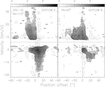
Figure 7: PV plot of the CO ($J$=1$\rightarrow$0) emission along the major axis of the molecular outflow A with PA$=115\degr$ (left), and of the outflow B with PA$=20\degr$ (right). The position offset is relative to the position of OVRO 1 (left) and relative to the center of symmetry of the outflow B, $\alpha$(J2000) = $20^{\rm h}07^{\rm h}05\aas@@fstack{s}38$, $\delta$(J2000) = $+27\degr 28^{\prime}59\aas@@fstack{\prime\prime}3$. Contours are $-1.2$, $-0.9$, $-0.72$, $-0.54$, $-0.36$, $-0.18$, 0.18, 0.36, 0.54, 0.72, 0.90, 1.2, 1.8, 2.7, 3.6, 4.5, and 5.4 Jy beam^-1. The horizontal line marks the systemic velocity, $V_{\rm LSR}=6$ km s^-1.

4.2.2 Physical parameters of the CO outflows

Table 4: Properties of the CO outflow

	$V^{a}$	$M^{b}$	$P^{c}$	$E^{c}$	$F_{\rm out}^{c}$
Lobe	(km s-1)	($M_{\odot}$)	($M_{\odot}$ km s-1)	($10^{44}$ erg)	($M_{\odot}\,\mbox{km s}^{-1}$ yr-1)
			OUTFLOW A
Blue	[$-19,+1$]	0.10	0.99	1.05	$2.8\times 10^{-4}$
Red	[$+11,+31$]	0.10	1.05	1.32	$2.5\times 10^{-4}$
Total		0.20	2.04	2.37	$5.3\times 10^{-4}$
			OUTFLOW B
Blue	[$-14,+1$]	0.02	0.23	0.24	$6.4\times 10^{-5}$
Red	[$+11,+19$]	0.03	0.19	0.14	$4.5\times 10^{-5}$
Total		0.05	0.42	0.38	$1.1\times 10^{-4}$

(a) Range of outflow velocities.
(b) Assuming an excitation temperature of 29 K.
(c) Momenta and kinetic energies are calculated relative to the cloud velocity, which is taken to be $V_{\rm LSR}=6$ km s^-1. Velocity not corrected for inclination.

Assuming that the CO emission is in LTE and is optically thin, the mass of the gas associated with the outflows detected in the region has been calculated by using Eq. 2 of Paper II. The high outflow velocities CO is expected to be optically thin (e.g. Arce & Goodman arce01 (2001)). If CO is optically thick in portions of the flow, the correction for opacity should be in any case small . As the CO spectra are complex and exhibit prominent self-absorption in both interferometric (see Fig. 5) and single-dish observations (Bachiller et al. bachiller95 (1995); Zhang et al. zhang05 (2005)), it is difficult to derive the excitation temperature from the CO brightness temperature. Therefore, taking into account the assumption of LTE, we have assumed that the excitation temperature is equal to the kinetic temperature of 29 K derived from NH₃ observations by Molinari et al. (molinari96 (1996)), a temperature slightly lower than the dust temperature derived by fitting the spectral energy distribution (SED) by Chini et al. (chini01 (2001)) but similar to the excitation temperature used for other intermediate-mass molecular outflows. We assumed an [H₂]/[CO] abundance ratio of 10⁴ (e.g., Scoville et al. scoville86 (1986)), and a $10\%$ Helium abundance. In Table 4 we give the mass, the momentum, kinetic energy, and momentum rate in the outflows, which have been estimated following the derivation of Scoville et al. (scoville86 (1986)). We also report the range of outflow velocities for the outflows. Note that the momentum, kinetic energy, and momentum rate in the outflow have not been corrected for the (unknown) inclination angle, $i$, of the flow with respect to the plane of the sky. In the case of correcting for inclination, the velocities should be divided by $\sin i$, and the linear size of the lobes by $\cos i$. It is almost impossible to separate the emission of both outflows for the SHV interval, especially close to the center of symmetry of the outflows (see previous section). Therefore, it is possible that some emission from outflow B has been counted as part of outflow A and vice-versa. As already mentioned in Paper II, due to some possible filtering of the emission by the interferometer, absorption of the emission by the ambient cloud, opacity effects, and the integration range chosen, the masses calculated should be considered as lower limits. The values of the mass, momentum, kinetic energy, and momentum rate are consistent with the values estimated from interferometric observations for other intermediate-mass molecular outflows (see Table 5). The dynamical timescales of the outflows, which have been estimated taking the ratio of the maximum separation of the outflow lobes and the terminal velocity of the outflow measured from the CO line wings, are 3000 and 5000 yr for the blueshifted and redshifted lobes of outflow A, and 5000 and 7000 yr for the blueshifted and redshifted lobes of outflow B.

4.3 The dense cores

4.3.1 Physical parameters of the dense cores

As can be seen in the spectra (Fig. 5) and the fitted parameters (Table 3), the gas towards OVRO 1 appears to be clearly at a different velocity, $V_{\rm LSR}$$\simeq$4.7 km s^-1, than OVRO 2 and OVRO 3, which have velocities of $V_{\rm LSR}$$\simeq$5.5–6 km s^-1.

Following Eq. 5 of Paper II, we estimated the virial mass of the sources assuming a spherical clump with a power-law density distribution $\rho\propto r^{-p}$, with $p=2.0$–1.5, and neglecting contributions from magnetic field and surface pressure (see Table 3). The virial masses have been computed from C¹⁸O, except for OVRO 1. For this source, it has been computed from HC₃N as it peaks close to OVRO 1 and is clearly associated with it. For OVRO 2, the emission is not resolved, and therefore one can only estimate an upper limit. The values estimated for OVRO 1, 4.3–5.7 $M_{\odot}$, are slightly lower than the mass derived from the continuum, 6.5 $M_{\odot}$. Taking into account that the mass of the central protostar has not been considered in this calculation, the total mass (circumstellar plus protostar) of OVRO 1 would be slightly higher than the virial mass. This would be consistent with the object undergoing collapse, and consistent with accretion driving the outflow. For OVRO 2, from the upper limits computed it is not possible to say whether the virial mass is higher or lower than the continuum mass. For OVRO 3, the virial mass estimated is clearly higher than the mass derived from the continuum. However, it is not possible to compare both masses as the C¹⁸O emission, from which the virial mass has been computed, is much more extended than the continuum emission, from which the circumstellar mass has been estimated.

4.3.2 Envelope mass from gas emission

As already mentioned in Paper II, the gas abundance relative to molecular hydrogen is the main uncertainty of the estimate of the mass of the molecular core. Therefore, instead of measuring the mass of the gas towards the protostars from the C¹⁸O or HC₃N emission, assuming a given fractional abundance of these species, it is better to estimate their fractional abundance from a comparison with the mass derived from the dust emission. We integrated the gas emission in the same area used to estimate the mass of the gas from the continuum dust emission, and assumed that the mass towards the continuum sources derived from C¹⁸O and HC₃N is that derived from the 2.7 mm continuum emission.

Following Eq. 3 and 4 of Paper II, the estimated C¹⁸O ($J$=1$\rightarrow$0) abundance relative to molecular hydrogen is $2.5\times 10^{-8}$ towards OVRO 1 and $\sim$ $5\times 10^{-8}$ towards OVRO 2 and OVRO 3. Typical C¹⁸O fractional abundances estimated towards molecular clouds are 1.7–4$\times 10^{-7}$ (Frerking et al. frerking82 (1982); Kulesa et al. kulesa05 (2005)). Therefore, even taking into account the uncertainties up to a factor of 5 introduced in the mass estimates by the different dust opacity laws used, the abundances derived towards OVRO 1, 2 and 3 are lower than the typical fractional abundances.

Regarding the HC₃N emission, the estimated abundance relative to molecular hydrogen is $1\times 10^{-10}$ towards OVRO 1, $6.5\times 10^{-11}$ towards OVRO 2, and $8.5\times 10^{-11}$ towards OVRO 3. The HC₃N abundance found in the literature can vary by up to 3 orders of magnitude, from $\sim$$3\times 10^{-11}$ (Vanden Bout et al. vandenbout83 (1983)) to $\sim$$10^{-8}$ (de Vicente et al. devicente00 (2000); Martín-Pintado et al. martin05 (2005)). Therefore, the HC₃N abundances derived towards OVRO 1, and especially those derived towards OVRO 2 and 3 are in the lower end of the range of fractional abundances estimated toward molecular clouds.

Table 5: Properties of intermediate-mass outflows derived from interferometric observations

	$d$	$L$	$M_{\rm env}$	$M_{\rm out}$	$F_{\rm obs}$	$t_{\rm dyn}$	NIR or
Outflow	(kpc)	($L_{\odot}$)	($M_{\odot}$)	($M_{\odot}$)	($M_{\odot}\,\mbox{km s}^{-1}$ yr-1)	($10^{3}$ yr)	MIRa,b	Ref.
IRAS 20343+4129 IRS1	1.4	1000–3200	0.8	10.04	$1.3\times 10^{-4}$	4.2	Y	1, 2
OMC1-S 137-408c	0.50		2	10.07	$1.2\times 10^{-2}$	0.11–3	N	3, 4, 5
L1206	0.91	1200	14.2	10.09	$7.7\times 10^{-5}$	8.0–20	Y	6, 7
Cepheus E	0.73	70	13.6	10.13	$2.3\times 10^{-4}$	4.0–8.0	Y	8, 9, 10
IRAS 21391+5802	0.75	235–500	5.1	10.14	$1.4\times 10^{-3}$	2.0–3.5	Y	11, 12, 13, 14, 15
IRAS 20050+2720 A	0.70	280	6.5	10.20	$5.3\times 10^{-4}$	6.5–7.3	?	16, 17, 18
OMC-2/3 MM7	0.45	76	0.36–0.72	10.34	$1.1\times 10^{-3}$	6.3–21	Y	19, 20, 21
IRAS 20293+3952 A	2.0	1050d	4	2.0	$2.1\times 10^{-2}$	4.3	N	1, 22, 23
IRAS 22171+5549	2.4	1800	25	2.7	$1.2\times 10^{-2}$	7	N	24, 25
IRAS 21307+5049	3.6	4000	53	3.2	$2.9\times 10^{-3}$	13	.Ne	24, 25
S235 NNW-SSE	1.8			4.0	$1.0\times 10^{-3}$	15–20	N	26, 27
S235 NE-SW	1.8	1000	16	9.0	$1.4\times 10^{-2}$	5.4–14.7	$?^{f}$	26, 27
IRAS 23385+6053	4.9	1500	61	10.6	$9.0\times 10^{-3}$	7.3	N	28, 29
HH 288c	2.0	500	6–30	11	$1.4\times 10^{-2}$	28	N	30

REFERENCES: 1: Sridharan et al.  (srid02 (2002)); 2: Palau et al. (2007b ); 3: Genzel & Stutzki (genzel89 (1989)); 4: Zapata et al. (zapata06 (2006)); 5: L. A. Zapata (private communication); 6: Crampton & Fisher (crampton74 (1974)); 7: Paper II; 8: Lefloch et al. (lefloch96 (1996)); 9: Moro-Martín et al. (moro01 (2001)); 10: Noriega-Crespo et al. (noriega04 (2004)); 11: Matthews (matthews79 (1979)); 12: Saraceno et al. (saraceno96 (1996)); 13: de Gregorio-Monsalvo (degregorio06 (2006)); 14: Paper I; 15: Getman et al. (getman07 (2007)); 16: Dame & Thaddeus(dame85 (1985)); 17: Froebrich (froebrich05 (2005)); 18: this work; 19: Takahashi et al. (takahashi06 (2006)); 20: Takahashi et al. (takahashi07 (2007)); 21: Nielbock et al. (nielbock03 (2003)); 22: Beuther et al. (2004a ); 23: Palau et al.  (2007a ); 24: Molinari et al.  (molinari02 (2002)); 25: Fontani et al. (2004a ); 26: Evans & Blair (evans81 (1981)); 27: Felli et al. (felli04 (2004)); 28: Molinari et al. (molinari98 (1998)); 29: Fontani et al.  (2004b ); 30: Gueth et al. (gueth01 (2001)).

(a) Y: source detected at $\lambda<8.0\leavevmode\nobreak\ \mu$m by the Infrared Array Camera (IRAC) of the Spitzer Space Telescope, ISOCAM at 7 $\mu$m, or by 2MASS; N: source not detected at $\lambda<8.0\leavevmode\nobreak\ \mu$m; ?: source for which the association between the millimeter and mid-infrared emission is dubious.
(b) The information was obtained either from the literature of from the Spitzer Science Center Data Archive interface Leopard.
(c) Because of the difficulty of treating each outflow separately, the parameters correspond to the whole emission, thus including the two outflows associated with OMC1-S 137-408 and with HH288.
(d) The luminosity of IRAS 20293+3952 is 6300 $L_{\odot}$. However, most of its luminosity comes from a B1 star ($L$$\sim 5250$ $L_{\odot}$: Panagia et al. panagia73 (1973)) associated with it and not from the intermediate-mass YSO powering the outflow A (Palau et al. 2007a ).
(e) Mid-infrared emission at 7 $\mu$m has been detected towards IRAS 21307+5049 by Fontani et al. (2004b ). However, the fact that the mid-infrared emission peak is offset by $\sim$6^′′ from the millimeter and submillimeter emission peaks led these authors to suggest that the mid-infrared data are likely due to the nearby cluster.
(f) Mid-infrared emission has been observed $1\aas@@fstack{\prime\prime}5$ to the south of the millimeter peak (Felli et al. felli06 (2006)). Such a separation is slightly greater than the error of the relative positions, and according to Felli et al. (felli06 (2006)) it cannot be firmly established whether both infrared and millimeter sources are related.

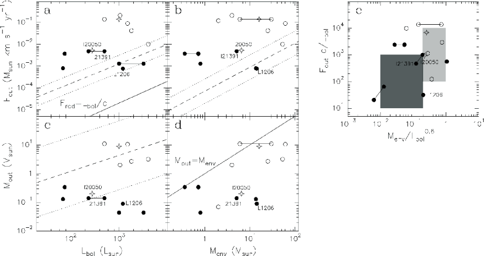
Figure 8: Correlations between source and outflow properties for the sample of intermediate-mass protostars and outflows listed in Table 5: (a) Outflow momentum flux $F_{\rm out}$ versus bolometric luminosity $L_{\rm bol}$. The ’best fit’ $F_{\rm out}$–$L_{\rm bol}$ correlation found for Class I sources by Bontemps et al. (bontemps96 (1996)) is plotted as a dashed line. Dotted lines represent the dispersion of the fit. The solid line presents the relation $F_{\rm out}=L_{\rm bol}/c$. (b) $F_{\rm out}$ versus circumstellar envelope mass $M_{\rm env}$. The ’best fit’ $F_{\rm out}$–$M_{\rm env}$ correlation found for a low-mass Class 0 and Class I sample by Bontemps et al. (bontemps96 (1996)) is plotted as a dashed line. Dotted lines represent the dispersion of the fit. (c) Outflow mass $M_{\rm out}$ versus $L_{\rm bol}$. The least square linear fit found for a sample of low- to high-mass sources by Wu et al. (wu04 (2004)) is plotted as a dashed line. Dotted lines represent the dispersion of the fit. (d)  $M_{\rm out}$ versus $M_{\rm env}$. The solid line presents the relation $M_{\rm out}=M_{\rm env}$. (e) $F_{\rm out}\,c/L_{\rm bol}$ (dimensionless) versus $M_{\rm env}/L_{\rm bol}^{0.6}$  ($M_{\rm env}$ and $L_{\rm bol}$ in units of $M_{\odot}$ and $L_{\odot}$). The light and dark grey boxes roughly denote the zones where the Class 0 and Class I sources, respectively, are located in Fig. 7 of Bontemps et al. (bontemps96 (1996)). The horizontal and oblique lines that join two dots indicate two different values for the same source or outflow property (see Table 5). Open circles represent sources not detected at $\lambda<8\leavevmode\nobreak\ \mu$m, filled circles represent sources detected at $\lambda<8\leavevmode\nobreak\ \mu$m, and stars represent sources for which the association between the millimeter and mid-infrared emission is dubious (see Table. 5). The three sources studied by us in Paper I, Paper II and this work are labeled.

5 Intermediate-mass protostars and their outflows

This present work, which is focused on the properties of IRAS 20050+2720 and of its molecular outflow, is the third of a series of high-angular resolution studies devoted to intermediate-mass protostars and their outflows, including the study of IRAS 21391+5802 (Paper I) and IRAS 22272+6358A (Paper II). We put the results on IRAS 20050+2720 in the context of our previous results, and in the context of intermediate-mass star formation. We further compare the properties and evolution of intermediate-mass protostars with those of their lower mass counterparts. We have compiled information on outflow properties that have been derived from interferometric observations in order to be sensitive to the same spatial scales and to better compare the properties with those derived for the sources in our study. Our sample is therefore not very homogeneous, as very few intermediate-mass outflows have been observed at high-angular resolution. In any case, we have been able to compile data of a total of 14 intermediate-mass protostars, including the 3 sources studied by us.

5.1 Multiplicity in intermediate-mass star-forming regions

The millimeter continuum emission around IRAS 20050+2720 has been resolved into three millimeter sources (see Fig. 1): an intermediate-mass source, OVRO 1, and two low-mass sources, OVRO 2 and OVRO 3. In addition, the powering source of outflow B has not yet been detected at millimeter wavelengths, or its emission has not been resolved from the extended emission of the circumstellar envelope surrounding the intermediate-mass OVRO 1 (see Sect. 3.2). If one also takes into account the millimeter source detected by Furuya et al. (furuya05 (2005)), located about $5^{\prime\prime}$ east of OVRO 1 and not resolved by our observations, the emission around IRAS 20050+2720 would be associated, at least, with 5 YSOs. And, except for OVRO 3 that could be associated with IRAS 20050+2720 and with the NIR source 5 detected by Chen et al. (chen97 (1997); see Sect. 3.1), none of them seems to be detected at infrared wavelengths yet. This situation very closely resembles the scenario around the intermediate-mass sources IRAS 21391+5802, in the bright-rimmed cloud IC 1396N, and IRAS 22272+6358A, in L1206, where the millimeter emission has been resolved into an intermediate-mass source surrounded by less massive and smaller objects (Paper I; Beltrán et al. 2004a ; Fuente et al. fuente07 (2007); Neri et al. neri07 (2007); Paper II). This suggests that intermediate-mass stars form in dense clustered environments. In other words, the formation of an isolated intermediate-mass star if existing appears rare. This is different from the low-mass case, where examples of protostars formed in relative isolation are known (e.g. L1157: Beltrán et al. 2004b ; HH 211: Palau et al. 2006a ; or Bok globules: Laundhart et al. laundhart97 (1997)). The crowded environments would explain the complexity of the immediate vicinity of intermediate-mass protostars.

Intermediate-mass protostars are associated with small protoclusters of low-mass millimeter sources, some of them not yet detected at shorter wavelengths. In many cases, they are also associated with young and embedded clusters of more evolved NIR sources (e.g. IRAS 21391+5802: Nisini et al. nisini01 (2001), Getman et al. getman07 (2007); L1206: Ressler & Shure ressler91 (1991), Kumar et al. kumar06 (2006); IRAS 20050+2720: Chen et a. chen97 (1997), Gutermuth et al. gutermuth05 (2005), Kumar et al. kumar06 (2006); S235: Felli et al. felli97 (1997); IRAS 22172+5549: Fontani et al. 2004a , Kumar et al. kumar06 (2006); IRAS 21307+5049: Fontani et al. 2004a ; IRAS 20293+3952 A: Palau et al. 2007a ). Interestingly, in some cases these NIR clusters contain a large number of more evolved low-mass Class II and Class III sources (e.g. IRAS 21391+5802: Getman et al. getman07 (2007), IRAS 20050+2720: Chen et al. chen97 (1997); IRAS 20293+3952 A: Palau et al. 2007a ; and possibly L1206: M. S. N. Kumar, private communication). This means that the intermediate-mass protostars and these more evolved low-mass sources cannot be coeval. All this suggests that, at least in some regions, intermediate-mass protostars would start forming after the first generation of low-mass stars has completed their main accretion phase. Such a situation appears to be typical of high-mass star-forming regions, where embedded massive stars that are still accreting material are surrounded by clusters of less embedded and more evolved low-mass Class I or Class II sources (Kumar et al. kumar06 (2006)).

The presence of multiple sources in intermediate-mass star-forming regions also explains the complex appearance of the molecular outflows in these regions when observed with low-angular resolution. This is due to, firstly, the presence usually of more than one outflow in the region (e.g. HH 288: Gueth et al. gueth01 (2001); IRAS 21391+5802: Paper I; IRAS 20050+2720: this paper), and secondly, to the stronger interaction of the outflow with the high-density clumps surrounding the intermediate-mass protostar (IRAS 21391+5802: Paper I). However, as shown by these studies of intermediate-mass star-forming regions, the molecular outflows, which are intrinsically more energetic than those driven by low-mass stars, are collimated and less complex when observed at high-angular resolution. In fact, they appear collimated even at low outflow velocities (Paper I, Paper II), similar to the low-mass protostellar flow in HH 211 (Gueth & Guilloteau gueth99 (1999); Palau et al. 2006b ).

5.2 Relationships between protostar properties and outflow parameters

Table 5 shows the properties of intermediate-mass outflows and their powering sources derived from interferometric observations, which have been compiled from the literature. Table 5 also gives information on whether the sources have been detected or not at NIR or mid-infrared (MIR) wavelengths. As seen in the table, only a very limited number of intermediate-mass outflows have been studied at high-angular resolution. In spite of the poor statistics of the sample, we compare the properties of intermediate-mass YSOs with those of low-mass protostars. To do this, we checked whether intermediate-mass YSOs are consistent with the correlations between source and outflow properties found for a sample of Class 0 and Class I protostars by Bontemps et al. (bontemps96 (1996)). In particular, we checked the correlation between circumstellar envelope mass $M_{\rm env}$ and the momentum rate in the outflow $F_{\rm out}$, the correlation between bolometric luminosity $L_{\rm bol}$ and $F_{\rm out}$, and that between the normalized momentum $F_{\rm out}\,c/L_{\rm bol}$ and $M_{\rm env}/L_{\rm bol}^{0.6}$  (see Fig. 8). Following Bontemps et al. (bontemps96 (1996)), we used the observed momentum rate in the outflow $F_{\rm obs}$ (see Table 5), corrected for inclination and opacity. We applied a mean correction factor of 2.9 for the inclination, corresponding to a mean inclination angle with respect to the plane of the sky of $\sim 32.7\degr$, and a mean correction factor of 3.5 for the opacity. Therefore, the corrected momentum flux of the outflow $F_{\rm out}$, is $F_{\rm out}\sim 2.9\times 3.5\times F_{\rm obs}\sim 10\times F_{\rm obs}$. For the three molecular outflows that had already been corrected for inclination angle $i$, we only applied the opacity mean correction factor 3.5. In addition, we also compared $M_{\rm env}$ and the mass of the outflow $M_{\rm out}$, and $L_{\rm bol}$ and $M_{\rm out}$. The different symbols in Fig. 8 indicates whether the sources have been detected at $\lambda<8\leavevmode\nobreak\ \mu$m or not, or whether the detection is dubious (see Table 5).

In Fig. 8$a$ and 8$b$, we compare the relationships between $F_{\rm out}$ and $L_{\rm bol}$ or $M_{\rm env}$  obtained for the intermediate-mass outflows with those obtained by Bontemps et al. (bontemps96 (1996)). The ’best fit’ correlation obtained by these authors is plotted as a dashed line, and the dispersion of the fit with dotted lines. As can be seen in the plot, intermediate-mass YSOs have, in general, higher $F_{\rm out}$ than low-mass objects. One could argue that this is due to the fact that the sources in our sample have been observed with interferometers while those of Bontemps et al. with single-dish. However, for those sources in our sample that have been observed with single-dish as well, the values of $F_{\rm out}$ derived are either comparable or even higher than those derived with interferometers. According to Eq. 5 of Bontemps et al. (bontemps96 (1996)), $F_{\rm out}$ is related to the accretion rate $\dot{M}_{\rm acc}$, the entrainment efficiency, and the outflow driving engine efficiency. Therefore, the higher $F_{\rm out}$ values suggest either a higher $\dot{M}_{\rm acc}$ for intermediate-mass stars, a higher entrainment efficiency or a higher outflow driving engine efficiency. Calvet et al. (calvet04 (2004)) have found, by means of optical and ultraviolet observations, that the average mass accretion rate for a sample of intermediate-mass T Tauri stars, which are the evolutionary predecessors of Herbig Ae stars, is a factor $\sim 5$ higher than that for their low-mass counterparts. Therefore, it is very likely that intermediate-mass YSOs accrete material faster. This seems a reasonable conjecture as these protostars have to gain enough mass before the circumstellar disks are dispersed. According to Fuente et al. (fuente01 (2001)), the dispersal of the circumstellar material and the end of the outflow activity should occur in $<10^{5}$ yrs.

As seen in Table 5 and Fig. 8, half of the sources have not been detected at $\lambda<8.0\leavevmode\nobreak\ \mu$m. This suggests that these sources, represented by open circles in Fig. 8, could be more deeply embedded in the core, and therefore to be in an earlier evolutionary stage than those detected and represented by filled circles. The difference in detection rate at NIR or MIR wavelengths is also evident in some source and outflow properties. Fig. 8 shows that for a similar $L_{\rm bol}$ or $M_{\rm env}$, the sources not detected at NIR or MIR wavelengths have higher, in some cases up to $\sim$2 orders of magnitude higher, $F_{\rm out}$ and $M_{\rm out}$ than those detected. Therefore, this suggests that the sources not detected at NIR or MIR wavelengths are more efficient at driving their outflows, which are more powerful, than those detected. The same happens when comparing $M_{\rm out}$ for objects with similar $L_{\rm bol}$  (see Fig. 8$c$). Those not detected at NIR or MIR wavelengths put more mass in the outflows than those detected. In addition, the non-detected sources agree better with the correlation between $M_{\rm out}$ and $L_{\rm bol}$  obtained by Wu et al. (wu04 (2004)) for a sample of low- to high-mass YSOs. Although the radiation pressure of the central source would not be enough to drive the outflow if the photons emitted by the central source were scattered only once, as shown by the fact that all the outflows have $F_{\rm out}$ above the radiative momentum flux $F_{\rm rad}=L_{\rm bol}/c$  (see Fig. 8$a$), $L_{\rm bol}$  of the central source and $M_{\rm out}$ are still correlated, showing the dependence of the outflow on its driving source. As seen in Fig. 8$d$, in general, the sources not detected at NIR or MIR wavelengths put almost the same amount of mass in the outflow as they have in the circumstellar envelope.

To further investigate these differences, we removed any luminosity dependence from both $F_{\rm out}$ and $M_{\rm env}$. Following Bontemps et al. (bontemps96 (1996)), we plotted the outflow efficiency $F_{\rm out}\,c/L_{\rm bol}$ versus $M_{\rm env}/L_{\rm bol}^{0.6}$  (Fig. 8$e$), along with the zones where the low-mass Class 0 and Class I sources are roughly located in Fig. 7 of Bontemps et al. (bontemps96 (1996)). This plot shows that, in general, the sources not detected at NIR or MIR wavelengths have a higher outflow efficiency. In the low-mass regime, there is a decline of the outflow efficiency with evolutionary stage (Bontemps et al. bontemps96 (1996)). Therefore, although we do not claim that the sources not detected at $\lambda<8.0\leavevmode\nobreak\ \mu$m are like low-mass Class 0 objects, we propose that these sources could be younger than those detected, as additionally suggested by the differences in properties such as $F_{\rm out}$, $M_{\rm out}$, and outflow efficiency. In the low-mass regime, the youngest protostars have been classified as Class 0 objects, based on criteria such as the ratio of submillimeter to bolometric luminosity, $L_{\rm submm}/L_{\rm bol}>5\times 10^{-3}$, where $L_{\rm submm}$ is measured longwards of 350 $\mu$m (André et al. andre93 (1993)). However, intermediate-mass star-forming regions are located, in general, at farther distances than low-mass ones, and usually associated with small clusters. Hence, the luminosity at wavelengths longwards of 350 $\mu$m will likely have contributions from other sources in the cluster, and therefore the criterion used to classify the youngest low-mass sources might not be applicable for intermediate-mass ones. In order to confirm this possible evolutionary difference in the sources of our sample, one should conduct a detailed source by source study of the SED at high-angular resolution, however, this goes beyond the scope of this work.

6 Conclusions

We studied the dust at 2.7 and 7 mm and the gas at 2.7 mm towards IRAS 20050+2720, an intermediate-mass YSO, with the OVRO Millimeter Array and the VLA. We also put the results on this and previously studied intermediate-mass sources in the context of intermediate-mass star formation.

The 2.7 mm continuum emission has been resolved into three sources, OVRO 1, OVRO 2, and OVRO 3. Two of them, OVRO 1 and OVRO 2, have also been detected at 7 mm. OVRO 3, which is located close to the C¹⁸O emission peak, could be associated with IRAS 20050+2720. The strongest source at millimeter wavelengths is OVRO 1, which has a deconvolved diameter of $\sim$$3\aas@@fstack{\prime\prime}3$ ($\sim$2300 AU) at the half-peak intensity contour of the dust emission. The source is surrounded by an extended and a fairly spherical halo or envelope, which has a size of $\sim$$11\aas@@fstack{\prime\prime}3$ ($\sim$8000 AU) at the 3 $\sigma$ contour level. OVRO 2 has a deconvolved diameter of $\sim$$2\aas@@fstack{\prime\prime}3$ ($\sim$1600 AU) at the half-peak intensity contour of the dust emission, and OVRO 3 is not resolved. The mass of the sources, estimated from the dust continuum emission, is 6.5 $M_{\odot}$ for OVRO 1, 1.8 $M_{\odot}$ for OVRO 2, and 1.3 $M_{\odot}$ for OVRO 3.

The multiplicity of sources observed towards IRAS 20050+2720, as well as towards IRAS 21391+5802 and L1206, appears to be typical of intermediate-mass star-forming regions. Intermediate-mass stars form in dense clustered environments, and in most cases they are associated with small protoclusters of low-mass millimeter sources, some of them not yet detected at shorter wavelengths. In many cases, as for example IRAS 20050+2720, IRAS 21391+5802 and L1206, intermediate-mass protostars are also associated with young and embedded clusters of more evolved NIR sources that sometimes contain a large number of more evolved low-mass Class II and Class III sources. This suggests that, at least in some regions, intermediate-mass protostars would start forming after the first generation of low-mass stars has completed their main accretion phase, a situation that appears to be typical of high-mass star-forming regions (Kumar et al. kumar06 (2006)).

The CO ($J$=1$\rightarrow$0) emission towards IRAS 20050+2720 traces two bipolar outflows within the OVRO field of view, a roughly east-west bipolar outflow, coincident with the outflow A of Bachiller et al. (bachiller95 (1995)) and apparently driven by the intermediate-mass source OVRO 1, and a northeast-southwest bipolar outflow, labeled outflow B and probably powered by a YSO engulfed in the circumstellar envelope surrounding OVRO 1. The outflow A presents a different morphology for the blueshifted and the redshifted emission. The blueshifted emission is more compact than the redshifted one. This lack of symmetry between the lobes could be due to the presence of the OVRO 3 core. High-angular resolution observations show that, in general, intermediate-mass outflows, which are intrinsically more energetic than those driven by low-mass YSOs, are not intrinsically more complex than low-mass outflows. Intermediate-mass outflows appear collimated, even at low velocities, and have properties that do not differ significantly from those of low-mass stars. $F_{\rm out}$ values of intermediate-mass protostars are higher than those of low-mass ones. Although one cannot discard a higher entrainment efficiency or outflow driving engine efficiency, this suggests that intermediate-mass YSOs very likely accrete material faster than low-mass ones.

Intermediate-mass protostars do not form a homogeneous group but have different properties. The sources not been detected at $\lambda<8.0\leavevmode\nobreak\ \mu$m clearly have higher $F_{\rm out}$, $M_{\rm out}$, and outflow efficiency than the sources detected at $\lambda<8.0\leavevmode\nobreak\ \mu$m for similar $M_{\rm env}$ and $L_{\rm bol}$. This suggests that the sources not detected at NIR or MIR wavelengths, which are likely more embedded in the core and drive more powerful outflows, could be in an earlier evolutionary stage.

- (1) André, P., Ward-Thompson, D., & Barsony, M. 1993, ApJ, 406, 122
- (2) Anglada, G., Rodríguez, L. F., & Torrelles, J. M. 1998a, in ASP Conf. Ser. 132, Star Formation with the Infrared Space Observatory, ed. J. L. Yun & R. Liseau (San Francisco: ASP), 303
- (3) Arce, H. G., & Goodman, A. A. 2001, ApJ, 554, 132
- (4) Bachiller, R. 1996, ARA&A, 34, 111
- (5) Bachiller, R., Fuente, A., & Tafalla, M. 1995, ApJ, 445, L51
- (6) Beltrán, M. T., Brand, J., Cesaroni, R., Fontani, F., Pezzuto, S., Testi, L., Molinari, S. 2006a, A&A, 447, 221
- (7) Beltrán, M. T., Girart, J. M., & Estalella, R. 2006b, A&A, 457, 865 (Paper II)
- (8) Beltrán, M. T., Girart, J. M., Estalella, R., Ho, P. T. P., & Palau, A. 2002, ApJ, 573, 246 (Paper I)
- (9) Beltrán, M. T., Girart, J. M., Estalella, R., & Ho, P. T. P. 2004, A&A, 426, 941
- (10) Beltrán, M. T., Gueth, F., Guilloteau, S., & Dutrey, A. 2004, A&A, 416, 631
- (11) Beuther, H., Schilke, P., & Gueth, F. 2004, ApJ, 608, 330
- (12) Bontemps, S., André, P., Terebey, S, & Cabrit, S. 1996, A&A, 311, 858
- (13) Briggs, D. 1995, Ph.D. Thesis, New Mexico Inst. Mining & Tech.
- (14) Calvet, N., Muzerolle, J., Briceño, C., Hernández, J. et al. 2004, ApJ, 128, 1294
- (15) Chen, H., Tafalla, M., Greene, T. P., Myers, P. C., & Wilner, D. J. 1997, ApJ, 475, 163
- (16) Chini, R., Ward-Thompson, D., Kirk, J. M., Nielbock, M., Reipurth, B., & Sievers, A. 2001, A&A, 369, 155
- (17) Choi, M., Panis, J.-F., & Evans II, N. J., 1999, A&ASS, 122, 519
- (18) Crampton, D., & Fisher, W. A. 1974, Publ. Dominion Ap. Obs. Victoria, 14
- (19) Dame, T. M., & Thaddeus, P. 1985, ApJ, 297, 751
- (20) de Gregorio-Monsalvo, I., Gómez, J. F., Suárez, O., Kuiper, T. B. H., Rodríguez, L. F., & Jiménez-Bailón, E. 2006, ApJ, 642, 319
- (21) de Vicente, P., Martín-Pintado, J., Neri, R., & Colom, P. 2000, A&A, 361, 1058
- (22) Evans; N. J. II, & Blair, G. N. 1981, ApJ, 246, 394
- (23) Frerking, M. A., Langer, W. D., & Wilson, R. W. 1982, ApJ, 262, 590
- (24) Felli, M., Massi, F., Navarrini, A., Neri, R., Cesaroni, R., & Jenness, T. 2004, A&A, 420, 553
- (25) Felli, M., Massi, F., Robberto, M., & Cesaroni, R. 2006, A&A, 453, 911
- (26) Felli, M., Testi, L., Valdettaro, R., & Wang, J.-J. 1997, A&A, 320, 594 2002, A&A, 420, 553
- (27) Fontani, F., Cesaroni, R., Testi, L., Molinari, S., Zhang, Q., Brand, J., & Walmsley, C. M. 2004a, A&A, 424, 179
- (28) Fontani, F., Cesaroni, R., Testi, L., Walmsley, C. M. et al. 2004b, A&A, 414, 299
- (29) Froebrich, D. 2005, ApJSS, 156, 169
- (30) Fuente, A., Ceccarelli, C., Neri, R., Alonso-Albi, T. et al. 2007, A&A, 468, L37
- (31) Fuente, A., Neri, R., Martín-Pintado, J., Bachiller, R., Rodríguez-Franco, A., & Palla, F. 2001, A&A, 366, 873
- (32) Furuya, R. S., Kitamura, Y., Wootten, A., Claussen, M. J., Kawabe, R. 2003, ApJSS, 144, 71
- (33) Furuya, R. S., Kitamura, Y., Wootten, A., Claussen, M. J., Kawabe, R. 2005, A&A, 438, 571
- (34) Genzel, R., & Stutzki, J. 1989, ARA&A, 27, 41
- (35) Getman, K., Feigelson, E. D., Garmire, G., Broos, P., & Wang, J. 2007, ApJ, 654, 316
- (36) Gueth, F., & Guilloteau, S. 1999, A&A, 343, 571
- (37) Gregersen, E. M., Evans, N. J. II, Zhou, S., & Choi, M. 1997, ApJ, 484, 256
- (38) Gueth, F., Schilke, P., & McCaughrean, M. J. 2001, A&A, 375, 1018
- (39) Gutermuth, R. A., Megeath, T., Pipher, J. L., Williams, J. P. et al. 2005, ApJ, 632, 397
- (40) Hildebrand, R. H. 1983, QJRAS, 24, 267
- (41) Hogerheijde, M. R., van Dishoeck, E. F., Blake, G. A., & van Langevelde, H. J. 1997, ApJ, 489, 293
- (42) Hogerheijde, M. R., van Dishoeck, E. F., Salverda, J. M., & Blake, G. A. 1999, ApJ, 513, 350
- (43) Kulesa, C. A., Hungerford, A. L., Walker, C. K., Zhang, X., & Lane, A. P. 2005, ApJ, 625, 194
- (44) Kumar, M. S. N., Keto, E., & Clerkin, E. 2006, A&A, 449, 1033
- (45) Laundhart,, R., & Henning, Th. 1997, A&A, 326, 329
- (46) Lefloch, B., Eislöffel, J., & Lazareff, B. 1996, A&A, 313, L17
- (47) Looney, L. W., Mundy, L. G., & Welch, W. J. 2000, ApJ, 529, 477
- (48) MacLeod, G. C., Scalise, E. Jr., Saedt, S., Galt, J. A., & Gaylard, M. J. 1998, AJ, 116, 1897
- (49) Martín-Pintado, J., Jiménez-Serra, I., Rodríguez-Franco, A., Martín, S., & Thum, C. 2005, ApJ, 628, L61
- (50) Matthews, T. J. 1979, A&A, 75, 345
- (51) Molinari, S., Brand, J., Cesaroni, R., & Palla, F. 1996, A&A, 308, 573
- (52) Molinari, S., Testi, L., Brand, J., Cesaroni, R., & Palla, F. 1998, ApJ, 505, L39
- (53) Molinari, S., Testi, L., Rodríguez, L. F., & Zhang, Q. 2002, ApJ, 570, 758
- (54) Moro-Martín, A., Noriega-Crespo, A., Molinari, S., Testi, L., Cernicharo, J., & Sargent, A. I. 2001, ApJ, 555, 146
- (55) Neri, R., Fuente, A., Ceccarelli, C., Caselli, P. et al. 2007, A&A, 468, L33
- (56) Nielbock, M., Chini, R., & Müller, S. A. H. 2003, A&A, 408, 245
- (57) Nisini, B., Massi, F., Vitali, Giannini, T. et al. 2001, A&A, 376, 553
- (58) Noriega-Crespo, A., Moro-Martín, A., Carey, S., Morris, P. W. et al. 2004, ApJSS, 154, 402
- (59) Ossenkopf, V., & Henning, Th. 1994, A&A, 291, 943
- (60) Palau, A. 2006, Ph.D. Thesis, Universitat de Barcelona
- (61) Palau, A., Estalella, R., Girart, J. M., Ho, P. T. P., Zhang, Q., & Beuther, H. 2007a, A&A, 465, 219
- (62) Palau, A., Estalella, R., Ho, P. T. P., Estalella, R. 2006b, A&A, 636, L137
- (63) Palau, A., Ho, P. T. P., Zhang, Q., Beuther, H., & Beltrán, M. T. 2007b, A&A, submitted
- (64) Palla, F., Brand, J., Cesaroni, R., Comoretto, G., & Felli, M. 1991, A&A, 246, 249
- (65) Panagia, N. 1973, AJ, 78, 929
- (66) Ressler, M. E., & Shure, M. 1991, AJ, 102, 1398
- (67) Richer, J., Shepherd, D. S., Cabrit, S., Bachiller, R., & Churchwell, E. 2000, in Protostars and Planets IV, ed. V. Mannings, A. Boss, & S. Russell (Tucson: University of Arizona Press), 867
- (68) Ridge, N. A., Wilson, T. L., Megeath, S. T., Allen, L. E., & Myers, P. C. 2003, AJ, 126, 286
- (69) Saraceno, P., et al. 1996, A&A, 315, L293
- (70) Scoville, N. Z., Carlstrom, J. E., Chandler, C. J., Phillips, J. A. et al. 1993, PASP, 105, 1482
- (71) Scoville, N. Z., Sargent, A. I., Sanders, D. B., Claussen, M. J., Masson, C. R., Lo, K. Y., & Phillips, T. G. 1986, ApJ, 303, 416
- (72) Shepherd, D. S. 2005, in Massive Star Birth: A Crossroads of Astrophysics, ed. R. Cesaroni, M. Felli, E. Churchwell, & M. Walmsley (Cambridge: Cambridge University Press), Proc. IAU Symp. 227, 237
- (73) Shepherd, D. S., & Churchwell, E. 1996a, 457, 267
- (74) Shepherd, D. S., & Churchwell, E. 1996b, 472, 225
- (75) Schneider, N., Bontemps, S., Simon, R., Jakob, H., Motte, F. et al. 2006, A&A, 458, 855
- (76) Sridharan, T. K., Beuther, H., Schilke, P., Menten, K. M.., & Wyrowski, F. 2002, ApJ, 566, 931
- (77) Takahashi, S., Saito, M., Takakuwa, S., & Kawabe, R. 2006, ApJ, 651, 933
- (78) Takahashi et al. 2007, in preparation
- (79) Vanden Bout, P. A., Loren, R. B., Snell, R. L., & Wootten, A. 1983, ApJ, 271, 161
- (80) Wilking, B. A., Mundy, L. G., Blackwell, J. H., & Howe, J. E. 1989, ApJ, 345, 257
- (81) Williams, J. P., & Myers, P. C. 1999, ApJ, 511, 208
- (82) Wu, Y., Wei, Y., Zhao, M., Shi, Y., Yu, W. et al. 2004, A&A, 426, 503
- (83) Zapata, L. A., Ho, P. T. P., Rodríguez, L. F., O’Dell, C. R., Zhang, Q., & Muench, A. 2006, ApJ, 653, 398
- (84) Zhang, Q., Hunter, T. R., Brand, J., Sridharan, T. K. et al. 2001, ApJ, 552, 167
- (85) Zhang, Q., Hunter, T. R., Brand, J., Sridharan, T. K. et al. 2005, ApJ, 625, 864