Collective atomic recoil laser as a synchronization transition

Abstract

We consider here a model previously introduced to describe the collective behavior of an ensemble of cold atoms interacting with a coherent electromagnetic field. The atomic motion along the self-generated spatially-periodic force field can be interpreted as the rotation of a phase oscillator. This suggests a relationship with synchronization transitions occurring in globally coupled rotators. In fact, we show that whenever the field dynamics can be adiabatically eliminated, the model reduces to a self-consistent equation for the probability distribution of the atomic “phases”. In this limit, there exists a formal equivalence with the Kuramoto model, though with important differences in the self-consistency conditions. Depending on the field-cavity detuning, we show that the onset of synchronized behavior may occur through either a first- or second-order phase transition. Furthermore, we find a secondary threshold, above which a periodic self-pulsing regime sets in, that is immediately followed by the unlocking of the forward-field frequency. At yet higher, but still experimentally meaningful, input intensities, irregular, chaotic oscillations may eventually appear. Finally, we derive a simpler model, involving only five scalar variables, which is able to reproduce the entire phenomenology exhibited by the original model.

I Introduction

Much progress has been recently made in understanding the onset of collective phenomena in cold atoms in the presence of a coherent electromagnetic field, when atomic recoil cannot be neglected. In particular, the experimental observation of collective atomic recoil laser (CARL) KCZC03 , accompanied by the development of simple theoretical models PYN02 has revealed that this is an appropriate physical environment for testing new and general ideas on the behaviour of globally coupled oscillators. In fact, the position of an atom moving along a line in a self-generated periodic potential can be interpreted as a phase: this observation opens up the possibility to compare CARL with other globally coupled systems KS75 ; BCM87 ; PRK96 and, in particular, with the Kuramoto model (KM) KuraBook . It is also interesting to explore the formal analogy with neural networks, which are currently the object of a strong research activity (see, e.g. abbott ; ZT04 ) in the perspective of unraveling the underlying information processing mechanisms. In fact, in one of the simplest, though non-trivial modeling schemes, neurons can be assimilated to rotators, since the action potential can be interpreted as a phase (this is, e.g., the case of the so called “leaky integrate and fire” neurons (LIF) abbott ). One of the goals of this manuscript is precisely to investigate analogies and differences between the collective phenomena that can arise in cold atoms and the synchronization phenomena that occur in general models of globally coupled rotators.

Altogether, the idea of atomic recoil is often linked with optical cooling CohenBook , but several years ago it was suggested that the recoil resulting from photon emission/absorption could induce macroscopic phenomena carl and possibly contribute to the transformation of kinetic energy into coherent light emission, in analogy to what happens in the free electron laser fel .

However, for a long time, progress on the theoretical side was hindered by the lack of a suitable model to describe the asymptotic stationary behavior of an ensemble of atoms. Preliminary experiments conducted at room temperature LBBT96 ; HBK96 were also partially inconclusive, as pointed out in BGGV97 . As a consequence, it was unclear which experimental conditions would be more appropriate for an experimental observation and even whether collective phenomena could be seen at all.

With the introduction of the first model capable of accounting for stationary phenomena PLP01 , it has been shown that at sufficiently low temperatures (above the region where quantum effects become important) an atomic-polarization grid can spontaneously arise, which triggers a coherent back-propagating field JLP03 . More recently, experimental evidence has been found KCZC03 and a corresponding theory has been proposed JPLP04 ; RPFBCZ04 ; CSKZCRPB05 , of collective atomic recoil lasing action in the presence of a very strong detuning, when the atomic dynamics can be effectively described by a linear response theory. Although a density grating arises in both cases, it is only in the latter setup that it contributes to generating the back-propagating field, while in the former one it just follows from the existence of two counterpropagating fields and it is not the dominant mechanism providing self-amplification.

So far, the only collective behaviour that has been observed is the spontaneous onset of a slightly-detuned backward-propagating constant field through a second order transition. In this paper, we extend the theoretical study, by first showing that the phase of the backward field can be eliminated by referring to a frame that moves with the instantaneous backward field frequency. This step allows uncovering an analogy with the KM, but also some relevant differences. In both CARL and KM, the force fields are self-consistently generated and depend on the non-uniformity in the probability distribution; moreover, both of them contain a mean-field sinusoidal term that eventually triggers ferromagnetic ordering. However, at variance with the “standard” KM, the slope of the potential (i.e. the effective frequency of the oscillators) is self-generated and there exists a preferred moving frame (the one we have accurately selected) where the dynamics is autonomous. This makes it meaningful to distinguish between locking (i.e. perfect synchrony) and libration, depending whether the potential exhibits local minima or not. The unavoidable presence of thermal noise introduces a further interesting effect, namely, a mismatch between the average velocity of the atoms and that of the density grating. This indeed represents the starting point for establishing a connection with another transition (see below).

By exploring the behaviour for larger but still experimentally accessible input intensities KCZC03 , we uncover an unexpectedly rich bifurcation scenario, starting from the primary transition which appears to be either second or first order, depending on the magnitude of the detuning between the injected field and the nearest cavity mode. More interesting is the secondary instability, which gives rise to amplitude oscillations of both the backward and forward field and is then followed by an unlocking transition, where the forward-field frequency too starts to be (red) detuned with respect to the input field. On the one hand, this regime is reminiscent of the periodic collective motion predicted in a model of charge density waves BCM87 , but it also resembles “self-organized” quasiperiodicity, a phenomenon first found in a model of LIF neuronsvanV , revisited in MP and proved in its fully generality in PR07 . We show that all these features and the transition to chaotic behaviour observed for yet higher input intensities are captured by a simple model containing only five variables. Such a model is derived in the limit of a strong cooperation parameter (see next section for its definition) and weak dipolar coupling, when the probability density is well approximated by the first Fourier mode. However, its validity appears to extend to a wide parameter region. The simplified model proves useful also to unravel the nature of the primary transition in the presence of a nonzero cavity-field detuning.

The paper is organized as follows: In section II, we derive the explicit form of the self-consistent washboard potential acting on the particle probability density and discuss the analogies with the Kuramoto model. In section III, we provide a full characterization of the various dynamical regimes appearing in this model. In section V, we derive a minimal model consisting of five ordinary differential equations, that is able to reproduce the rich phenomenology of the full system. Finally, in section VI, we summarize the main results and comment about the open problems.

II The model

The original CARL model carl considers only the dynamics of the back-scattered field. Such approximation is valid in the vicinity of the first threshold, but it fails at higher input intensities. It becomes then necessary to consider the forward mode dynamics as well, as first proposed in BRM97 and further discussed in YN01 ; PYN02 . Besides, as analyzed in JPLP04 , different models should be invoked, depending on the physical mechanisms that are responsible for atomic thermalization. For instance, if the process involves collisions (with either an external buffer gas, or hard boundaries), a Vlasov equation with a BGK-type collisional operator BGK54 for the atomic density in phase space BV96 is appropriate to model the thermalization. This leads to a Vlasov-type equation for the evolution of the density of probability. On the other hand, in the context of cold atoms dynamics, thermalization can be achieved via Doppler cooling cool . Then, each cooling cycle changes slightly the atomic momentum, and the appropriate thermalization model, as shown in CohenBook , may therefore be a Fokker-Planck operator RiskenBook , to describe the interaction between the probability distribution of particles and the molasses fields.

In this latter case, the model consists of a set of two equations for the complex cavity fields $x_{b}$, $x_{f}$, coupled to a Fokker-Planck equation for the single particle probability distribution $Q(\theta,p)$ for the atomic position $\theta$ and momentum $p$. Like in Ref. JPLP04 , we limit ourselves to considering the strong friction limit, which is both physically meaningful and allows to obtain some analytical results.

Accordingly, under the simplifying hypothesis of a vanishingly small inertia, the model reduces to a Fokker-Planck equation for the density $\rho(u,\overline{t})$ of atoms in the position $u$, accompanied by two equations for the complex amplitudes $x_{f}$, $x_{b}$ of the forward and backward field, respectively

$$\partial_{\overline{t}}\rho = -\nu\partial_{u}\Im(x_{f}x_{b}^{\star}{\rm e}^{2iu})\rho+T\partial^{2}_{u}\rho,$$

$$\frac{d{x}_{f}}{d\overline{t}} = -\kappa(1+i\Delta)x_{f}+\kappa Y-i\kappa Cx_{b}\langle{\rm e}^{-2iu}\rangle,$$ (1)

$$\frac{d{x}_{b}}{d\overline{t}} = -\kappa(1+i\Delta)x_{b}-i\kappa Cx_{f}\langle{\rm e}^{2iu}\rangle,$$

where the adimensional parameters have the following meaning: i) $C$ is the atom-field coupling constant; ii) $\Delta$ is the suitably shifted (forward) field-cavity detuning; iii) $\nu$ is the dipolar coupling; iv) $T$ is the atomic temperature; v) $Y$ is input field amplitude; vi) $\kappa^{-1}$ is the photon lifetime within the ring cavity, rescaled to the coherence time of the atomic transition.

We find it convenient to further rescale the variables, into $t=\kappa\overline{t}$, $x_{f}=YF$, $x_{b}=YB$, and $u=z/2$ (which implies $\rho(u,t)=2P(z,t)$). Accordingly, the model reads,

$$\partial_{t}P = -\mu\partial_{z}\Im(FB^{\star}{\rm e}^{iz})P+\sigma\partial^{2}_{z}P,$$

$$\dot{F} = -(1+i\Delta)F+1-iCB\mathcal{R}^{\star},$$ (2)

$$\dot{B} = -(1+i\Delta)B-iCF\mathcal{R},$$

where the dot denotes the derivative with respect to the new time variable $t$, and we have explicitly introduced the order parameter,

$$\mathcal{R}(t)=\int_{0}^{2\pi}dz{\rm e}^{iz}P(z,t).$$ (3)

Moreover, we defined the two effective control parameters $\mu=2Y^{2}\nu/\kappa$ and $\sigma=4T/\kappa$. As a result, it turns out that there are four relevant parameters that cannot be scaled out, namely, the detuning $\Delta$, the so-called cooperation parameter $C$, the input intensity $\mu$, and the temperature $\sigma$.

II.1 A moving frame

Next, we perform yet another change of variables to remove an irrelevant variable (a phase) from the dynamics. We do that by referring to a moving frame

$$\theta=z+\alpha(t),$$ (4)

where $\alpha$ is to be defined. The new probability density writes,

$$Q(\theta,t)=P(z,t).$$ (5)

Additionally, we introduce an amplitude-and-phase description for the two fields

$$F = f{\rm e}^{i\phi},$$

$$B = b{\rm e}^{i\beta}.$$

Notice that with these notations, a positive (negative) linear growth of the phases is to be interpreted as a red (blue) shift in the field frequency. Accordingly, the Fokker-Planck equation reads,

$$\partial_{t}Q=-\partial_{\theta}\left[\dot{\alpha}+\mu fb\sin(\phi-\beta-\alpha+\theta)\right]Q+\sigma\partial^{2}_{\theta}Q.$$

This equation suggests defining

$$\alpha\equiv\phi-\beta.$$ (6)

By doing so, we obtain

$$\partial_{t}Q=-\partial_{\theta}\left[\dot{\phi}-\dot{\beta}+\mu fb\sin\theta\right]Q+\sigma\partial^{2}_{\theta}Q.$$ (7)

Moreover, the order parameter writes,

$$\mathcal{R}={\rm e}^{i(\beta-\phi)}R{\rm e}^{i\psi}$$ (8)

where

$$R{\rm e}^{i\psi}\equiv R_{c}+iR_{s}=\int d\theta{\rm e}^{i\theta}Q(\theta,t)$$ (9)

As a result, the field equations write as

$$\dot{f} = \cos\phi-f-CbR_{s},$$ (10)

$$\dot{b} = -b+CfR_{s},$$ (11)

$$\dot{\phi} = -\frac{\sin\phi}{f}-\frac{CbR_{c}}{f}-\Delta,$$ (12)

$$\dot{\beta} = -\frac{CfR_{c}}{b}-\Delta.$$ (13)

We can now replace the expression for $\dot{\phi}$ and $\dot{\beta}$ in the Fokker-Planck equation to finally obtain,

$$\partial_{t}Q=-\partial_{\theta}\left[C\frac{f^{2}-b^{2}}{fb}R_{c}-\frac{\sin\phi}{f}+\mu fb\sin\theta\right]Q+\sigma\partial^{2}_{\theta}Q,$$ (14)

from which we see that the variable $\beta$ does not play any role in the dynamics, since it does not contribute to any of the force fields. Accordingly, we conclude that the model is fully described by the three equations (10,11,12) plus the Fokker-Planck equation (14). Upon interpreting $\theta$ as a phase, we can recognize atoms as a rotators and the underlying dynamics as that of identical globally coupled rotators in the presence of noise. The mutual interaction is mediated by the two fields $F$ and $B$ which follow their own dynamics. The primary interest in this setup was motivated by the possible existence of a regime where the modulus of the order parameter (as well as the amplitude of the backward field) is different from zero. In view of the above relationship with rotator systems, the onset of this regime is akin to a synchronization transition. However, it is also interesting to notice some analogies with the standard laser threshold. In fact, in both cases the frequency of the backward field is self-generated by the dynamics, but the corresponding phase does not contribute to the dynamics itself. Accordingly, from a mathematical point of view, the transition appears to be a degenerate Hopf bifurcation. Moreover, from the above equations, it turns out that the reference frame moves with a velocity equal to the frequency difference between the two fields. In dimensional variables this means that the frame velocity is $2(\dot{\phi}-\dot{\beta})/k$, where $k$ is the wavenumber of the injected field.

II.2 The physical parameter range

In order to keep contact with a possible experimental confirmation, we give here the meaningful orders of magnitude of the four relevant parameters, making reference to the experiment carried out in Ref. KCZC03 . The cavity is characterized by a power transmission coefficient of the cavity mirrors $\mathcal{T}=6.3\;10^{-6}$ and a roundtrip length $\Lambda=8.5\;\text{cm}$. Accordingly, the cavity linewidth is $\kappa=-c/\Lambda\ln(R)\sim 22$ kHz. The atomic sample consists of ${}^{85}\text{Rb}$ atoms whose temperature and density are $T_{0}=250\mu$K and $n=3\;10^{17}\text{m}^{-3}$, respectively. The characteristic length of the atomic sample is $L=10^{-3}\text{m}$. The optical parameters are given by the coherence dephasing rate of the D1 transition, namely, $2\gamma_{\perp}=\gamma_{\parallel}=5.9$MHz. The dipolar moment is $\mathcal{D}=1.5\;10^{-29}\text{cm}^{-1}$. The detunings between the injected field and both the atomic transition and the nearest cavity mode are $\Delta_{a}=1$ THz and $\Delta_{c}\sim 0$, respectively. Therefore, the physical expressions and the relative orders of magnitude of the parameters are

$$C= \frac{\alpha L}{\mathcal{T}} \mathcal{O}(1-10^{2}),$$

$$\Delta= \Delta_{c}+C \pm\mathcal{O}(0-10),$$

$$\sigma= \frac{k^{2}k_{B}T_{0}}{m\kappa^{2}\gamma_{\perp}^{2}} \mathcal{O}(10^{-1}-10^{1}),$$

$$\mu= \frac{Y^{2}\bar{\gamma}\Omega}{2\gamma K^{2}\Delta_{a}} \mathcal{O}(0-10),$$

where $\alpha$ is the unsaturated absorption rate per unit length, $k_{B}$ is the Boltzman constant, and $m$ the atomic mass.

III Stationary states

Both in the perspective of determining the stationary solution and to emphasize the analogies with the KM, we derive an adiabatic CARL model (ACM) by setting the time-derivatives of the three field variables equal to zero. In order to keep the notations as simple as possible, initially we assume $\Delta=0$ (see Section V for the qualitative changes induced by a nonzero detuning). From Eq. (11)

$$b=CR_{s}f.$$ (15)

By then setting to zero the derivative in Eq. (12), we obtain

$$\sin\phi=-C^{2}fR_{s}R_{c},$$ (16)

while, from Eq. (10),

$$\cos\phi=f(1+C^{2}R_{s}^{2}).$$ (17)

By combining together these last two equations, one obtains

$$f^{-2}=C^{4}R_{s}^{2}R_{c}^{2}+(1+C^{2}R_{s}^{2})^{2}.$$

After replacing back into the equation for $Q(\theta,t)$, the model reduces to

$$\partial_{t}Q=-\partial_{\theta}\left[\omega(1+\xi\sin\theta)\right]Q+\sigma\partial^{2}_{\theta}Q,$$ (18)

where

$$\omega = \frac{R_{c}}{R_{s}}$$ (19)

$$\xi = \frac{\mu CR_{s}^{2}}{R_{c}\left[(1+C^{2}R_{s}^{2})^{2}+C^{4}R_{s}^{2}R_{c}^{2}\right]}$$ (20)

Since the field dynamics is absent, the model resembles a typical Fokker-Planck equation in a static potential, as studied extensively by Risken RiskenBook , except that the force field is here determined self-consistently from some moments of the distribution $Q$. The structure of the force field corresponds to that of the so-called Adler, or washboard, potential adler . The parameters $\omega$ and $\xi$ respectively measure the tilt and modulation amplitude of the potential. The tilt originates from our choice of a moving frame: a stationary solution for the probability density would indeed correspond to a moving grating in the laboratory frame. The second parameter $\xi$ quantifies the amplitude of the entraining force on the atomic could. For $\xi\leq 1$, the drifting velocity is simply modulated, but it does not change sign. For $\xi\geq 1$, the washboard potential possesses a local minimum and complete entrainment (synchronization) is possible.

III.1 The zero temperature limit

In order to understand the underlying physics, it is convenient to start from the zero-noise limit. A priori, the two most symmetric solutions are: (i) the perfectly synchronized state with all particles located in the same position; (ii) the so-called splay state NW92 , characterized by a constant flux of particles.

If all particles are located in $\theta$, then $(R_{c},R_{s})=(\cos\theta,\sin\theta)$ and we can reduce the whole problem to the ordinary differential equation

$$\dot{\theta}=\frac{\cos\theta}{\sin\theta}+\frac{\mu C\sin^{2}\theta}{1+C^{2}(2+C^{2})\sin^{2}\theta}.$$ (21)

The fixed point solution of the fully synchronized state is obtained by determining the zero of the force field,

$$\cos\theta\bigg{[}1+C^{2}(2+C^{2})\sin^{2}\theta\bigg{]}=-\mu C\sin^{3}\theta.$$ (22)

By squaring it and introducing $X=\sin^{2}\theta$, we obtain the equation

$$(1-X)\bigg{[}1+C^{2}(2+C^{2})X\bigg{]}^{2}=\mu^{2}C^{2}X^{3}.$$ (23)

It is easy to verify that there exists a meaningful solution for any value of the parameters $C$ and $\mu$. This means that, at zero temperature, any arbitrarily small input field is able to trigger a backward field that is sufficiently strong to entrain the atoms in the fully synchronized state.

On the other hand, the splay state is obtained by imposing that, at zero temperature, the flux is constant, i.e. $\partial_{\theta}[(\omega(1+\xi\sin\theta))Q]=\partial_{t}Q\equiv 0$. The probability density then becomes proportional to the inverse of the force field,

$$Q(\theta)=\frac{N}{\omega(1+\xi\sin\theta)},$$ (24)

where $N$ is a normalization condition. From the definition of the order parameter, Eq. (3), we obtain the condition,

$$R_{c}+iR_{s}=\int d\theta\frac{{N\rm e}^{i\theta}}{\omega(1+\xi\sin\theta)}.$$ (25)

By solving the real part of this integral, one easily finds that $R_{c}=0$. Accordingly, from Eq. (19), it follows that $\omega=0$ which means that there cannot be any tilt and, as a consequence, no splay state, because the flux would be necessarily equal to zero.

III.2 A comparison with the Kuramoto model

At zero temperature, there exists a nontrivial collective state for arbitrarily small input field. At finite temperature, as already shown in Ref. JPLP04 , there exists a threshold value for the input intensity, below which, the noise washes out any order.

The presence of such transition, as well as the underlying structure of the model are reminiscent of what observed in KM. In the absence of quenched disorder (i.e., assuming that all rotators are identical), KM writes,

$$\partial_{t}Q=-\partial_{\theta}KR\sin(\theta-\psi)Q+\sigma\partial^{2}_{\theta}Q,$$ (26)

where $K$ denotes the coupling constant, while the other notations are the same as before. It is well known that the order parameter $R$ is larger than zero only if the coupling constant is larger than some critical value which depends on the noise strength.

From the comparison between ACM and KM, one can notice that the sinusoidal force depends on the local phase in ACM, while it depends on the phase difference in KM. This implies that the dynamics of the KM is time independent in any moving frame (as long as the velocity is constant). It is nevertheless convenient to write the evolution equation in the frame which allows removing the drift term (which is indeed absent in the KM). On the other hand, the drift term cannot be removed from the ACM without introducing an explicit time-dependence. A last difference concerns the amplitude of the sinusoidal force which is proportional to the order parameter in KM, while it is strongly nonlinear, in the ACM, due to the coupling between order parameter and field equations as it can be seen in Eqs. (19,20). It is now important to understand the implications of such differences on the observed dynamics, especially in the presence of stochastic processes, when phase-transitions are expected.

III.3 The type of synchronization

In the vicinity of the primary transition, the backward field intensity is arbitrarily small. Therefore, $\xi$ is also a small quantity and the washboard potential cannot drag the atomic cloud. All the variables being stationary, the flux is constant in the vicinity of the transition, and the collective behavior is a typical splay state. In order to understand how this regime connects with the fully synchronous state observed in the zero-noise limit, we solve numerically Eqs. (10,11,12,14) for different temperature values. As illustrated in Fig. 1a, there is no backward field for large enough $\sigma$, while the forward field intensity is constant and equal to 1 with our normalizations. Upon decreasing $\sigma$ below the threshold value, $f$ drops below 1 (dashed line), while $b$ increases from zero (solid line) and, at small temperatures, decreases again in this particular case. At the same time, the amplitude of the order parameter increases monotonously from 0 to 1 (dot dashed line). Note that the highest backward field does not correspond to the most coherent state ($R=1$), because of the nonlinear dependence of the potential amplitude on the order parameter. At the same time, in Fig. 1b, we see that for decreasing $\sigma$, the relative amplitude $\xi$ of the modulation increases above 1 (meaning that the potential exhibits local minima) and eventually decreases, though remaining larger than 1 at zero temperature, when there is complete dragging.

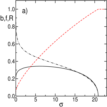
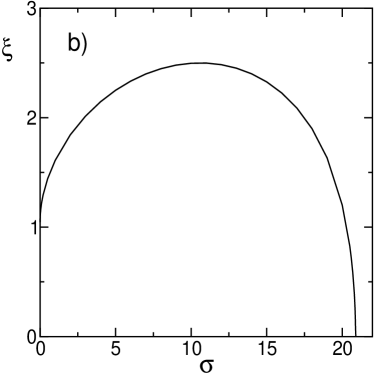
Figure 1: (color online) Left panel: Bifurcation diagram of the ACM model for $\mu=40$, $C=5$, $\Delta=0$. Solid, dashed, and dotted-dashed lines correspond to $b$, $f$, and $R$ as a function of $\sigma$. Right panel: the parameter $\xi$ of the force field.

On the other hand, we see in Fig. 2, that the velocity of the density grating, which is given by $-\omega$ (solid line), decreases monotonously with $\sigma$. In the same figure, the dashed line corresponds to the average velocity $v$ of the atoms, that is given by

$$v_{a}=-\omega+2\pi\Phi$$ (27)

where $\Phi$ is the stationary flux of the Fokker-Planck equation

$$\Phi\equiv\omega Q(0)-\sigma\partial_{\theta}Q(0).$$ (28)

By comparing the two curves, we see that the density grating velocity is everywhere larger than the atomic velocity except at zero temperature, where the two coincide, sign of a complete dragging. The difference is maximal in the vicinity of the primary transition, where the atomic velocity is nearly zero (because the backward field is negligible too), while the grating velocity is maximal.

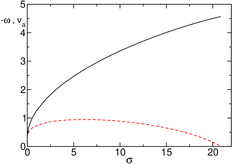
Figure 2: (color online) Velocity of the density grating ($-\omega$, solid line) and average velocity of the atoms ($v_{a}$, dashed line) versus the scaled temperature $\sigma$ and the same parameter values as in Fig. (1).

In order to check the generality of this scenario, we present in Fig. 3 a phase diagram for different values of both $\sigma$ and the input intensity $\mu$. There we see that above the transition line, there are two broad areas that extend down to $\sigma=0$. In the first one (color-shaded, for larger values of $\mu$), the potential has minima, and there is no fixed point. In the second one, (in white, between the transition line and the dashed line), the potential has no minima. The dashed line separating these two regions does not represent a true transition line, but marks a quantitative difference. above (first region), the flux is triggered by the noise, since the barrier to the right of a minimum is lower than that on the left; below (second region), the flux is intrinsically deterministic.

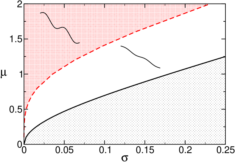
Figure 3: (color online) Phase diagram separating locked/drifting from partially locked regimes for $C=5$.

IV Numerical analysis

So far we have discussed the stationary state that arises from the solution of the ACM. We have shown the existence of two phases: i) a trivial one characterized by a zero order parameter and an independent evolution of the single atoms; ii) a collective state characterized by two different velocities for the single atoms and the density grating. This scenario is superficially reminiscent of that one found in the KM, but the properties of the collective motion are slightly more subtle. In the frame where the dynamics is stationary, there is still a non-zero flux induced by a finite tilting, that cannot be removed. However, there are further differences. At variance with the KM, here we show the existence of more complicated dynamical regimes that appear when the amplitude of the injected field is further increased beyond the primary transition. In Fig. 4, we show the typical sequence of states that are detected upon increasing the input field $\mu$.

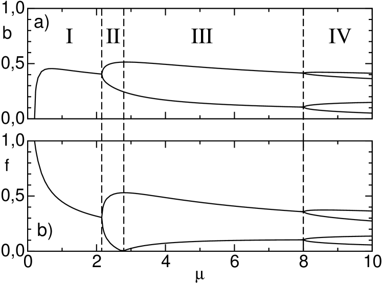
Figure 4: Bifurcation diagram for the backward (panel a) and forward (panel b) field amplitudes as a function of $\mu$. The other parameters are $C=20$, $\sigma=1$, and $\Delta=0$. The meaning of the various regions is discussed in the text.

For each value of $\mu$, the extrema of the field are plotted. Inside region $I$, there is only one point, meaning that the collective state is stationary in the moving frame. A secondary Hopf bifurcation separates region $I$ from region $II$, where the two field amplitudes start oscillating. In region $II$, the average frequency of the forward field still remains locked to that of the input field. This can be appreciated in Fig. 5a,d where we plot the real and imaginary components of the order parameter ($R_{c}$, $R_{s}$) and of the forward field ($f_{c}$, $f_{s}$) for $\mu=2.3$. In fact, neither $R$, nor $F$ exhibit an overall rotation since, in both representations, the limit cycle does not encircle the origin. Upon further increasing $\mu$, an unlocking occurs: in region $III$, the periodic oscillation amplitudes are accompanied by a rotation, as it can be seen in Fig. 5b,e, where both limit cycles projections now encircle the origin for $\mu=6$ (see Sec. IV.2 for details). Finally, a period doubling bifurcation signals the appearance of yet more complicated dynamical states and the possible onset of a chaotic dynamics. This occurs in region $IV$ and can be appreciated by looking at Fig. 5c,f, where the phase state projections are plotted for $\mu=9$.

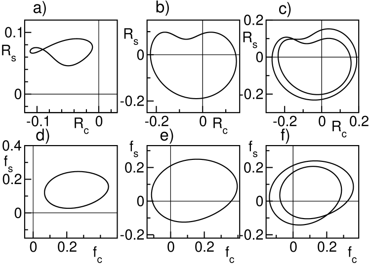
Figure 5: Phase space portraits of the typical behaviour observed in region $II$ (panels a,d, $\mu=2.3$), III (panels b,e, $\mu=6$) and region $IV$ (panels c,f $\mu=9$). Parameters are those of Fig. (4).

IV.1 The secondary transition

Besides solving directly the Fokker-Planck equation, we have determined the locus of the secondary Hopf bifurcation, by first determining the steady state in terms of a continued fraction expansion as described in JPLP04 . The equilibrium probability distribution has been evaluated analytically by using its integral form (see e.g. RiskenBook for further details); the stability analysis has been thereby carried out by introducing infinitesimal perturbations for the fields and for the probability distribution, by referring to an equispaced mesh containing $N\sim 256$ points. Finally, we have determined the eigenvalues of a sparse Jacobian matrix of size $(N+3)^{2}$ by means of the QR decomposition meshchach while the integral form of the equilibrium distribution has been evaluated by using the Clenshaw-Curtis quadrature integration scheme Flam .

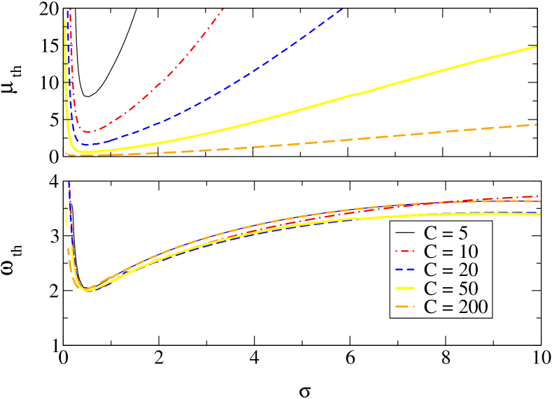
Figure 6: (color online) Locus of the secondary Hopf bifurcation as a function $\mu$ and $\sigma$, for different values of $C$. As $C$ decreases, the threshold for self-oscillation goes toward infinite values of $\mu$.

The main results are summarized in Fig. 6. There, one can see that the secondary bifurcation is inhibited at small temperatures, where both the threshold power $\mu_{h}$ and the Hopf frequency $\omega_{h}$ diverge to infinity. This inhibition also takes place for small values of the cooperation parameter $C$.

Furthermore, it is worth noticing the limiting behavior of the secondary threshold as $C$ is increased: All bifurcation curves tend to accumulate on an asymptote. Besides, the frequency of the secondary bifurcation is almost independent of $C$. This suggests that in the large-$C$ limit, the parameter $C$ can be scaled out of the problem. In fact, in the next section we show that it is convenient to introduce the smallness parameter $1/C$ and thereby suitably expand the dynamical equations.

Depending on the temperature value $\sigma$, we have found that the secondary bifurcation can be either super- or sub-critical, as it can be appreciated in Fig. 7 where a narrow but increasing region of bistability can be identified for the two larger $\sigma$ values. The diagrams have been obtained by sweeping the control parameter $\mu$ both in the increasing and decreasing direction, while keeping constant the parameters $C=20$ and $\Delta=0$.

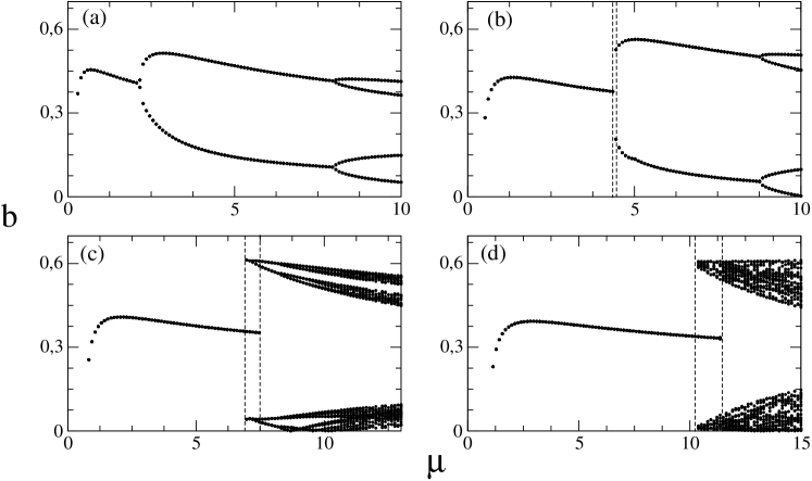
Figure 7: Bifurcation diagram for the backward field amplitude $b$ as a function $\mu$. the fixed parameters are $C=20$ and $\Delta=0$. Panels (a),(b),(c), and (d) correspond to $\sigma=1,2,3$ and $4$, respectively. As $\sigma$ increases, a region of bistability indicated by the vertical dashed lines, becomes more and more visible thus indicating a subcritical secondary Hopf bifurcation.

Finally, in order to clarify whether the field dynamics is a necessary ingredient for the richness of the observed phenomenology, we artificially reintroduced the photon lifetime into the field equations by multiplying their time derivatives by $\kappa$. The field dynamics can thereby be adiabatically eliminated in the limit $\kappa\rightarrow\infty$. By running extensive numerical simulations, we have found that when $\kappa$ increases, the Hopf bifurcation occurs for diverging values of both $\mu$ and $\sigma$. This provides an indirect indication that field dynamics is a necessary ingredient for observing the essential features of the bifurcation scenario.

IV.2 The unlocking transition

The most intriguing transition is that one separating region $II$ from region $III$. If one looks at the projection of the limit cycle of $F$ in the complex plane ($f_{s}$, $f_{c}$), a crossing of the origin appears for a specific $\mu$-value where $F$ is instantaneously equal to 0. This can be seen in Fig. 8.

Since the $F$ dynamics is a limit cycle, it can be considered as a closed, oriented curve in the complex plane ($f_{s}$, $f_{c}$). It is thus possible to assign to it a winding number $n$ around the origin of the complex plane. In turns, this allows to define the average frequency of $F$ as $2\pi n/T$ where $T$ is the period of the cycle. Therefore, the regimes in region $II$ and region $III$ are characterized by a zero and non zero average rotation, respectively. One can consider intituively that the mechanism responsible for the red shift of the backward field with respect to the input field is at some point responsible for shifting the forward field with respect to the frequency of the backward one.

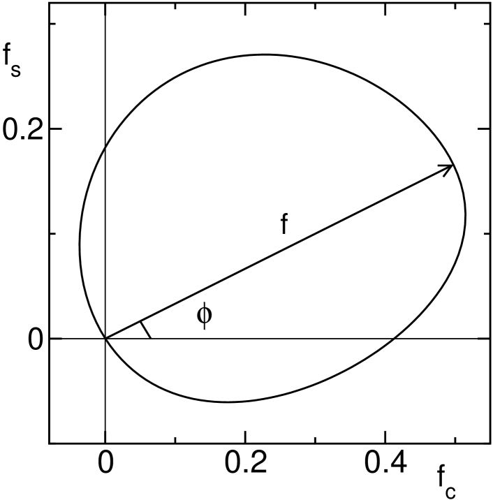
Figure 8: A projection of $F$ in the complex plane, for the critical value $\mu_{c}=2.752$, when the forward field unlocks from the input field. Parameters are those of Fig. (4). The cycle goes through the point $F=0$.

A less trivial scenario is found in the ($R_{c}$, $R_{s}$) plane (see Fig. 9): only a fraction of the limit cycle remains unchanged when passing from below to above the transition point. The remaining part is made of two complementary halves of a circumference, so that across the transition, the whole limit cycle abruptly encircles the origin, thus signaling the onset of an order-parameter rotation.

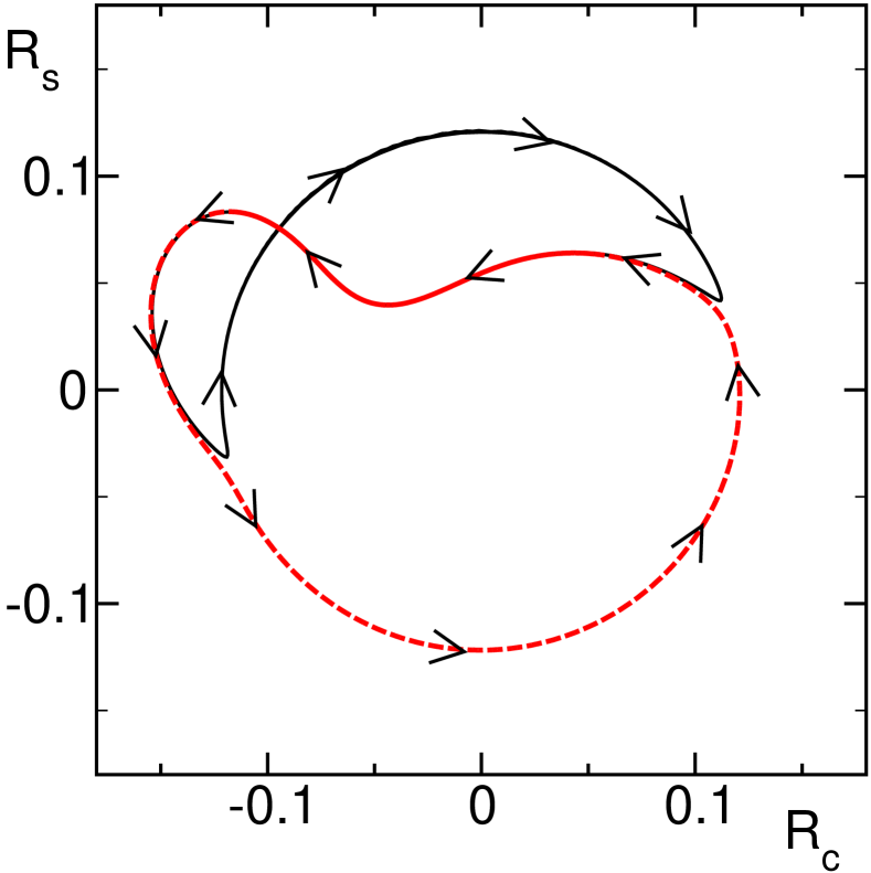
Figure 9: (color online) A projection of two limit cycles just below and above the critical point, $\mu_{c}=2.752$ where the forward field unlocks from the input field. The other parameter values are those of Fig. 5. The arrows indicate the direction of the motion: below (above) the transition, in the (un)locked regime, the upper (lower) semicircle is followed.

In order to further clarify the transition, let us look at the evolution of the potential tilt $\dot{\phi}-\dot{\beta}$.

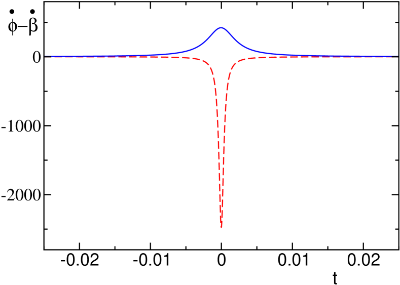
Figure 10: (color online) The behavior of the instantaneous slope of the potential, just below ($\mu=2.75$ dashed line) and above ($\mu=2.76$ the transition point). The different amplitude of the two curves is due to a different distance from the critical point. Parameters are those of Fig. (4).

In Fig. 10 we see that in the vicinity of the singular point, where the field amplitude $f$ is close to zero (for the sake of simplicity, we have set the origin of the time axis such that the minimal distance from the origin occurs at $t=0$), $\dot{\phi}-\dot{\beta}$ becomes very large, but the sign of this quantity is different above and below the transition, because the origin is encircled only above the transition. In the laboratory frame, however, the average velocity of the atoms exhibits a smooth change across the transition; in fact, the discontinuous variation of the instantaneous frequency is compensated by a discontinuous variation of the flux – cf. Eq. (27). Finally, in Fig. 11 we show the dependency of the average frequency of both the forward ($\overline{\dot{\phi}}$), and the backward ($\overline{\dot{\beta}}$) field, as a function of $\mu$.

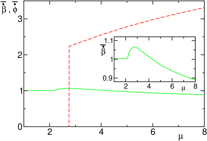
Figure 11: (color online) Frequency of the forward (dashed line) and backward (solid line) fields, referred to that of the input field, as a function of $\mu$. Parameters are the same as in Fig. 4. An enlargement of the $\overline{\dot{\beta}}$ behaviour is plotted in the inset.

There, we can see that both frequencies have the same sign and that the red-shift of the forward field is larger than the one of the backward field. Both features can be understood by means of the following heuristic argument. We indeed expect that the same mechanism that is responsible for the red shift of the backward field with respect to the input field should, at some point (when the backward field intensity is large enough) be responsible for red-shifting the forward field with respect to the backward one. This is precisely what we see.

V A minimal model

In this section we go back to the general case $\Delta\neq 0$ and show how the model can be reduced to a set of five ordinary differential equations that is still able to reproduce the relevant phenomenology discussed in the previous section. We start by assuming that the parameter $C$ is large and introduce the smallness parameter $\varepsilon\equiv C^{-1/3}$. As a next step, we perform the following change of variables, that has been suggested by numerical simulations,

$$t = \varepsilon\tau,$$

$$f = \varepsilon u\qquad b=\varepsilon v.$$ (29)

Moreover, we express the probability density $Q(\theta,t)$ as the sum of a homogeneous component and a sinusoidal perturbation, namely,

$$Q(\theta,t)=\frac{1}{2\pi}+\varepsilon^{2}S(\theta,\tau)$$ (30)

and correspondingly define

$$R_{s}=\varepsilon^{2}r_{s}\qquad R_{c}=\varepsilon^{2}r_{c}.$$ (31)

Accordingly, the equations for the field variables write,

$$\frac{du}{d\tau} = \cos\phi-\varepsilon u-vr_{s},$$

$$\frac{dv}{d\tau} = -\varepsilon v+ur_{s},$$

$$\frac{d\phi}{d\tau} = -\frac{\sin\phi}{u}-\frac{vr_{c}}{u}-\varepsilon\Delta,$$ (32)

$$\frac{d\beta}{d\tau} = -\frac{ur_{c}}{v}-\varepsilon\Delta.$$

while the Fokker-Planck equation writes,

$$\partial_{\tau}S = -\frac{\mu\varepsilon}{2\pi}uv\cos\theta-\partial_{\theta}\left[\mathcal{D}\omega+{\mu\varepsilon^{3}uv}\sin\theta\right]S$$ (33)

$$+\sigma\varepsilon\partial^{2}_{\theta}S.$$

where we have introduced

$$\mathcal{D}\omega=\frac{d\phi}{d\tau}-\frac{d\beta}{d\tau}=r_{c}\left(\frac{u}{v}-\frac{v}{u}\right)-\frac{\sin\phi}{u}$$ (34)

both to keep the notations as compact as possible and to remind that $\beta$ is not a relevant variable.

So far, no approximation has been introduced, and the above two sets of equations are equivalent to the initial formulation. However, we can recognize the existence of small terms when $\varepsilon$ is small. In particular, it is tempting to neglect all terms which are proportional to some (positive) power of $\varepsilon$, but this limit is singular. In fact, the resulting model is dissipationless (notice also that all physical parameters would disappear). On the one hand, the diffusion term in the Fokker-Planck equation disappears as well as the position dependent force, so that any initial condition for the distribution $S(\theta)$ remains invariant in time, what is not physical. On the other hand, the field dynamics is conservative as well (the two loss terms vanish). Since, finally, as we see below, there are conserved quantities, it is obvious that any arbitrarily small dissipation is going to qualitatively modify the asymptotic behavior and we, accordingly, cannot drastically set the $\varepsilon$ terms equal to zero. Nevertheless, we are entitled to neglect the cubic term, what is less crude an hypothesis. The resulting simplified Fokker-Planck equation can be solved exactly, assuming that $S(\theta)$ reduces to its first Fourier mode. It is convenient to express the amplitude of such mode directly referring to the two components of the order parameter,

$$S(\theta)=\frac{1}{2\pi}[(r_{c}+ir_{s})e^{-i\theta}+c.c.]$$ (35)

We indeed obtain (from now on, we again use a dot to mean the derivative with respect to the time variable $\tau$)

$$\dot{r}_{c} = -\frac{\mu\varepsilon}{2}uv-\mathcal{D}\omega r_{s}-\sigma\varepsilon r_{c}$$

$$\dot{r}_{s} = \mathcal{D}\omega r_{c}-\sigma\varepsilon r_{s}$$ (36)

which complement the first three equations in Eqs. (32)

If we now pass to phase and amplitude

$$r_{c}=r\cos\delta\qquad r_{s}=r\sin\delta$$ (37)

the entire set of equations writes

$$\dot{u} = \cos\phi-\varepsilon u-vr\sin\delta,$$

$$\dot{v} = -\varepsilon v+ur\sin\delta$$

$$\dot{\phi} = -\frac{rv}{u}\cos\delta-\frac{\sin\phi}{u}-\varepsilon\Delta,$$ (38)

$$\dot{\delta} = \mathcal{D}\omega+\frac{\mu\varepsilon}{2}\frac{uv}{r}\sin\delta,$$

$$\dot{r} = -\sigma\varepsilon r-\frac{\mu\varepsilon}{2}uv\cos\delta$$

while

$$\mathcal{D}\omega=r\cos\delta\left(\frac{u}{v}-\frac{v}{u}\right)-\frac{\sin\phi}{u}$$ (39)

Let us now discuss an analogy between our asymptotic limit and the small gain approximation, or the Uniform Field Limit (UFL), that are widely used in laser physics. Our approach implicitly assumes a weak action of the fields onto the atomic sample, i.e. a small dipolar coupling. Therefore, the Bragg grating imprinted onto the atomic density can be considered as a small perturbation of a homogeneous sample. On the other hand, one has to assume that the retroaction of the atoms onto the cavity is sufficiently strong for the small density modulation to influence the fields, i.e. a large cooperation parameter $C$. This approximation can be compared for instance with the small gain approximation, where one assumes that the material gain is simply proportional to its population inversion. This amounts to neglecting nonlinear saturation processes such as power broadening for a two-level atoms or carrier heating for a semiconductor material. Altogether, the asymptotic limit of this section is analogous to the UFL which amounts to considering a weak single pass gain within the cavity and, simultaneously, small optical losses, in such a way that a finite net amplification can eventually occur.

V.1 Numerical and theoretical analysis

V.1.1 The primary transition with non-zero detuning

Analytic expressions for the steady states of Eqs. (38) are derived in the appendix. The resulting bifurcation diagrams corresponding to $\Delta=0$, 2, 3, and -2, respectively, are displayed in Fig. 12, where, for the sake of clarity, we keep using the same notations as in the previous section. In particular, we see that for positive and large enough detuning there exist two branches (besides the trivial one $b=0$). This means that the primary bifurcation becomes subcritical, signaling the appearance of a bistability region. Still from the analytic discussion presented in the appendix, it turns out that the primary threshold is

$$\mu_{th}=\frac{1+\Delta^{2}}{C}\left[\Delta(\sigma-1)+(\sigma+1)\sqrt{\Delta^{2}+4\sigma}\right],\\$$ (40)

It is important to notice that this expression holds true also for the original model, since in the vicinity of the transition, the behaviour of $Q(\theta)$ is by definition dominated by the first Fourier harmonic.

As shown in the appendix, it is possible to derive an analytic expression for the saddle-node bifurcation, which turns out to be,

$$\mu_{sn}=\frac{2}{C}\frac{\left(2\Delta\sigma-\Delta^{3}\right)\sqrt{\Delta^{2}+4\sigma}+\Delta^{4}+2\sigma^{2}}{\sqrt{\Delta^{2}+4\sigma}-\Delta}.$$ (41)

Notice that this equation makes sense only when both solutions of the biquadratic equation (55) are positive. This can happen only for $\Delta$ larger than a critical value $\Delta_{c}$ that can be determined by setting $\mu_{sn}=\mu_{th}$,

$$\Delta_{c} = \frac{1}{\sqrt{\sigma_{c}+1}}.$$ (42)

Thus, one can conclude that, when $\Delta$ is negative, no bistability can occur, while it is allowed for a sufficiently large positive detuning.

Finally, in the small temperature limit, the minimum threshold is achieved for a detuning

$$\Delta_{m} = 2\frac{(1-\sigma)\sqrt{\sigma}}{1+9\sigma+8\sigma^{2}}.$$ (43)

Fig. 13 shows the spinodal decomposition of the solutions curve in the $(\Delta,\mu)$ plane of both the original and the simplified model (see dashed and solid lines, respectively) for $\sigma=1$ and $C=20$. One can see that there is a reasonable agreement even though the corresponding $\varepsilon$-value is not too small ($\sim 0.36$). The two shaded regions correspond to the mono- and the bistable regime, respectively. The full circle marks the tricritical point, where the bistable area appears in the original model.

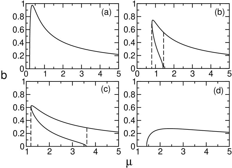
Figure 12: Bifurcation diagram of the steady states of Eqs. (38) as a function of $\mu$, for $C=20$ and $\sigma=1$. Panels (a),(b),(c), and (d) correspond to $\Delta=0$, 2, 3, and -2, respectively. The dashed lines denote the border of the bistability regions whenever there is one.

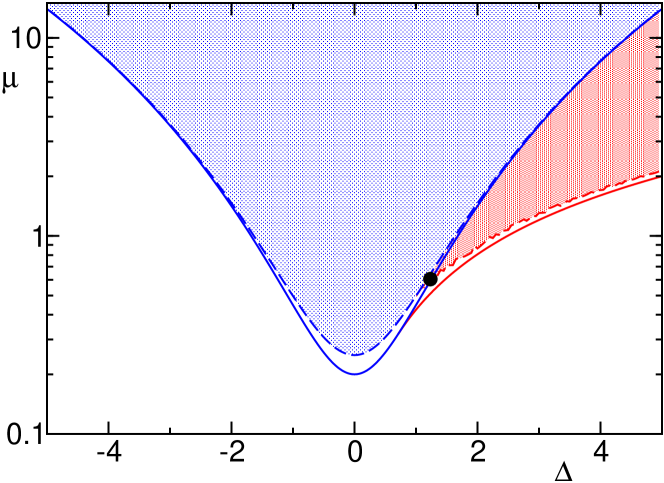
Figure 13: (color online) Spinodal decomposition of the steady states. Dashed lines refer to the original full model (for $\sigma=1$ and $C=20$); solid lines refer to the simplified model (38). The two shaded regions correspond to mono and bistable regimes in the full model. The circle denotes the tricritical point $\Delta_{c}$.

V.1.2 The secondary transition

The almost quantitative agreement between the full and the simplified model is not solely restricted to steady states. At larger input intensities, the simplified model exhibits a scenario that is much reminiscent of that observed in the original model: a secondary instability is first detected, that is followed by the unlocking phenomenon and, finally, by a sequence of period doubling bifurcations towards a chaotic regime. This indicates that the degrees of freedom that are responsible for the onset of macroscopic order are the very same ones leading to the self-pulsating instability. In order to confirm whether the simplified model is really built on the relevant physical variables, we have investigated whether the locus of the secondary transition exhibits a similar dependence on the control parameters. We proceded along the same lines described in Sec. IV.1. Our main results are summarized in Fig. 14. There, one can see that the characteristics of the full model described in Fig. 6 are preserved, like e.g., inhibition of the transition for small values of either the temperature or the cooperation parameter $C$. By comparing the full and dashed lines in Fig. 14, one can also notice that an almost quantitative agreement with the full model is obtained whenever the value of $\mu_{th}$ is not too large. Otherwise, the approximation, that consists in truncatiing the Fourier expansion of the probability distribution after the first mode, breaks. The overall quantitative agreement is reasonably good for values down to $C=50$, regardless of the value of the temperature $\sigma$.

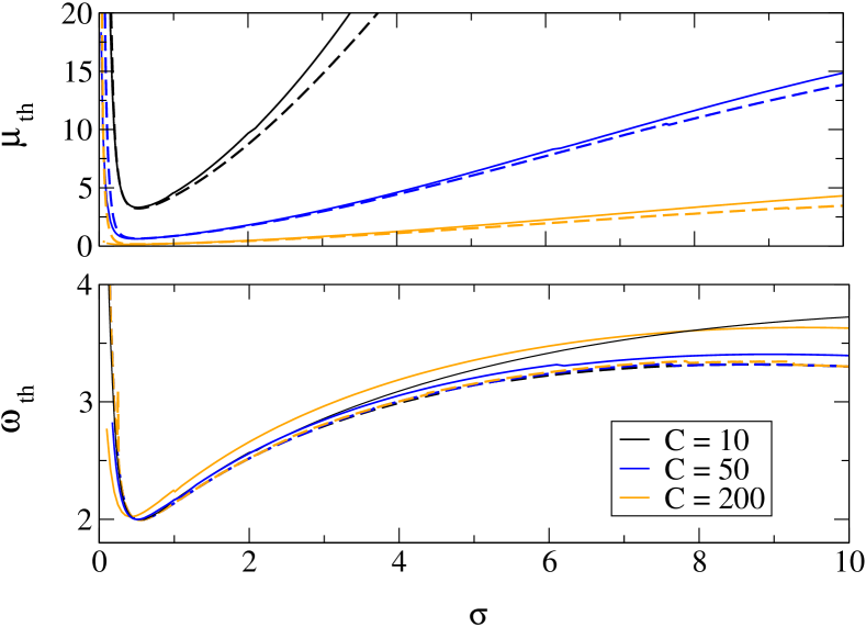
Figure 14: (color online) Locus of the secondary instability as a function $\mu$ and $\sigma$, for different values of $C$. Predictions of the simplified model, Eqs. (38) with dashed lines, are compared with those of the exact model, Eqs. (10)-(14), with solid lines. Parameters are those of Fig. 6

V.2 The $C\to\infty$ limit

Since the highest degree of dynamical complexity amounts to a sequence of period-doubling bifurcations, one might wonder whether it is possible to further reduce the dimensionality of the model from five to three degrees of freedom. In order to clarify this question we now consider the limit $\varepsilon\rightarrow 0$ and, for the sake of simplicity, we restrict the analysis to the resonant case $\Delta=0$. It is, unfortunately, necessary to perform a further change of variables; namely we introduce

$$u_{c}=u\cos\phi\qquad;\qquad u_{s}=u\sin\phi$$ (44)

and

$$v_{c}=v\cos(\delta-\phi)\qquad;\qquad v_{s}=v\sin(\delta-\phi)$$ (45)

The resulting equations read

$$\dot{r} = -\varepsilon\sigma r-\frac{\mu\varepsilon}{2}(v_{c}u_{c}-v_{s}u_{s})$$

$$\dot{u_{c}} = 1-rv_{s}-\varepsilon u_{c}$$

$$\dot{u_{s}} = -rv_{c}-\varepsilon u_{s}$$ (46)

$$\dot{v_{c}} = ru_{s}-\varepsilon v_{c}-\frac{\mu\varepsilon}{2}\frac{v_{s}}{r}(v_{s}u_{c}+v_{c}u_{s})$$

$$\dot{v_{s}} = ru_{c}-\varepsilon v_{s}+\frac{\mu\varepsilon}{2}\frac{v_{c}}{r}(v_{s}u_{c}+v_{c}u_{s})$$

The great advantage of this representation is that in the $\varepsilon\to 0$ limit, it factorizes into three independent and partially degenerate blocks

$$\dot{r} = 0$$

$$\ddot{u}_{c} = -r^{2}u_{c}$$ (47)

$$\ddot{u}_{s} = -r^{2}u_{s}$$

characterized by three constants of motion,

$$\mathcal{C}_{1} = r$$

$$\mathcal{C}_{2}^{2} = (v_{s}-1/r)^{2}+u_{c}^{2}$$ (48)

$$\mathcal{C}_{3}^{2} = v_{c}^{2}+u_{s}^{2}$$

Accordingly, a general solution writes as

$$v_{s} = \frac{1}{\mathcal{C}_{1}}+\mathcal{C}_{2}\sin(\mathcal{C}_{1}t+\eta_{1})$$

$$u_{c} = \mathcal{C}_{2}\cos(\mathcal{C}_{1}t+\eta_{1})$$

$$v_{c} = \mathcal{C}_{3}\sin(\mathcal{C}_{1}t+\eta_{2})$$ (49)

$$u_{s} = \mathcal{C}_{3}\cos(\mathcal{C}_{1}t+\eta_{2})$$

from which it is clear that two other constants enter the game, namely the phases $\eta_{1}$, and $\eta_{2}$. However, one phase can be removed by shifting the origin of the time axis, namely by introducing the phase difference $\eta=\eta_{2}-\eta_{1}$. Thus, we see that altogether, it should be possible at least to remove one out of the 5 variables. However, rather than pursuing this goal, we prefer to limit our discussion to the problem of determining the value of all the relevant constants. In order to do that, it is necessary to reintroduce a finite smallness parameter $\varepsilon$ and thereby determining the time derivative of the various “constants”. By denoting with a prime the derivative with respect to $\varepsilon\tau$, we find

$$\mathcal{C}^{\prime}_{1} = -\sigma\mathcal{C}_{1}-\frac{\mu}{2}\mathcal{C}_{2}\mathcal{C}_{3}\sin\eta$$

$$\mathcal{C}^{\prime}_{2} = -\mathcal{C}_{2}+\frac{\mu\mathcal{C}_{3}}{16\mathcal{C}_{1}^{3}}\left[(\mathcal{C}_{2}^{2}-\mathcal{C}_{3}^{2})\mathcal{C}_{1}^{2}-4\right]\sin\eta$$ (50)

$$\mathcal{C}^{\prime}_{3} = -\mathcal{C}_{3}-\frac{\mu\mathcal{C}_{2}}{16\mathcal{C}_{1}^{3}}\left[(\mathcal{C}_{2}^{2}-\mathcal{C}_{3}^{2})\mathcal{C}_{1}^{2}+4\right]\sin\eta$$

$$\eta^{\prime} = -\frac{\mu}{16\mathcal{C}_{1}^{3}}\left[(\mathcal{C}_{2}^{2}+\mathcal{C}_{3}^{2})\mathcal{C}_{1}^{2}+4\right]\left(\frac{\mathcal{C}_{3}}{\mathcal{C}_{2}}+\frac{\mathcal{C}_{2}}{\mathcal{C}_{3}}\right)\cos\eta$$

These equations admit a pair of symmetric fixed points which correspond to a periodic dynamics in the original variables,

$$\eta=\pm\frac{\pi}{2}\quad\mathcal{C}_{1}=\pm\left(\frac{\mu}{4}\right)^{1/3}\quad\mathcal{C}_{2}^{2}=\mathcal{C}_{3}^{2}=\frac{\sigma}{2}\left(\frac{4}{\mu}\right)^{2/3}$$ (51)

Therefore, the most robust dynamics which persists in the $C\to\infty$ limit, is the periodic one, arising after the Hopf bifurcation.

VI Conclusion

By recasting a known CARL model as a self-consistent equation for the probability distribution, we have been able to discuss analogies and differences with the Kuramoto model for synchronization in ensemble of globally coupled rotators. In fact, although the primary transition, giving rise to the spontaneous formation of a density grating, resembles the onset of a macroscopic synchronized state in the Kuramoto model, there are important differences. In particular, the global coupling affects the frequency of the oscillators (here, the velocity of the atoms), determining the tilting of the effective washboard potential. Another difference concerns the existence, in the CARL context, of an “absolute” reference frame, the only one where the equations are time-independent. As a result of these differences, we find a subtlety in the macroscopic behaviour: the average velocity of the grating does not coincide with the average velocity of the single atoms. Such a feature is reminiscent of the collective behaviour discussed in PR07 , where it is shown that nonlinear all-to-all interactions may lead to the onset of a peculiar periodic macroscopic phase. That phase is (in the absence of external noise) both characterized by a microscopic quasi-periodic motion and an average frequency of the single oscillators that differs from the period of the macroscopic motion. However, the correspondence between this behaviour and the collective atomic motion arising beyond the primary threshold is perhaps incomplete, since in the CARL context, the periodic global dynamics reduces to a fixed point in the “absolute” reference frame. A more promising candidate to establish a full analogy is the periodic motion arising beyond the unlocking transition, although the presence of microscopic stochastic fluctuations makes it difficult to formulate a convincing final statement. In fact, on the one hand, quasiperiodicity can be recognized as such only in deterministic systems, and, on the other hand, we are aware of at least another mechanism leading to periodic oscillations in globally coupled noisy rotators (see, e.g. BCM87 ). Unfortunately, in the context of cold atoms, we cannot consider directly the zero-noise limit, as it corresponds to a qualitatively different regime, namely full synchronization. Therefore, until an objective criterion of distinguishing possibly different classes of periodic collective motions will be introduced, the problem will remain open.

Finally, we wish to recall that the rich phenomenology extensively discussed in this paper is experimentally accessible, since we have everywhere (with the only exception of the zero-temperature limit) considered parameter values that are compatible with the experiment discussed in KCZC03 . The only important constraint comes from the need to stabilize and control a priori of the frequency of the input field, without the help of any feedback coming from the output of the cavity itself as done in Ref. KCZC03 .

Appendix

In this appendix we determine the steady states of Eqs. (38), by setting all the derivatives equal to zero. From the second and the last of them, one obtains

$$\sin\delta = \frac{\varepsilon v}{ur}$$

$$\cos\delta = -\frac{2\sigma r}{\mu uv}$$ (52)

By now subtracting the fourth from the third equation in the set (38) and thereby eliminating $\sin\delta$ and $\cos\delta$ with the help of Eq. (52), we obtain a biquadratic equation in $s=v/r$. Such an equation has always one and only one positive, and thus physically acceptable, solution,

$$\frac{\varepsilon\mu}{2}s^{2}=-\frac{\Delta}{2}+\frac{\Delta}{2}\sqrt{\Delta^{2}+4\sigma}.$$ (53)

By now squaring and summing the two expressions for $\sin\delta$ and $\cos\delta$ in (52) we find that the intensity of the forward field is

$$u^{2}=\varepsilon^{2}s^{2}+\frac{4\sigma^{2}}{\mu^{2}}\frac{1}{s^{2}}$$ (54)

The last step consists in solving the first and third equation in (38) for $\cos\phi$ and $\sin\phi$, respectively, squaring and summing. As a result, we obtain a biquadratic equation for $r$,

$$c_{4}r^{4}+c_{2}r^{2}+c_{0}=0$$ (55)

where

$$c_{4} = \varepsilon^{2}s^{4}+\frac{4\sigma^{2}}{\mu^{2}}$$

$$c_{2} = 2u^{2}\varepsilon\left(\varepsilon s^{2}-\frac{2\Delta\sigma}{\mu}\right)$$

$$c_{0} = u^{2}\left(\varepsilon^{2}u^{2}(1+\Delta^{2})-1\right)$$

The bifurcation point of the homogeneous state $r=0$ is found by setting $c_{0}=0$. With the help of Eqs. (54,53), this condition transforms into Eq. (40), displayed in Sec. V.

Moreover, the above biquadratic equation may have two distinct nontrivial solutions. The critical point where a pair of solutions is created (the saddle-node bifurcation) can be determined by imposing

$$c_{2}^{2}-4c_{4}c_{0}=0$$ (56)

With the help of Eqs. (54,53), this condition transforms into Eq. (41). Notice that this condition makes sense only when the two resulting solutions are both larger than zero, i.e. when $c_{2}/c_{4}<0$. Finally, from the way the solutions have been derived, one can observe a curious property: the two branches are characterized by the same amplitude of the forward field!