INSTITUT NATIONAL DE RECHERCHE EN INFORMATIQUE ET EN AUTOMATIQUE

Tournament MAC with Constant Size Congestion Window for WLAN
Jérôme Galtier, Orange Labs N° 6396
December 2007

Abstract: In the context of radio distributed networks, we present a generalized approach for the Medium Access Control (MAC) with fixed congestion window. Our protocol is quite simple to analyze and can be used in a lot of different situations. We give mathematical evidence showing that our performance is tight, in the sense that no protocol with fixed congestion window can do better. We also place ourselves in the WiFi/WiMAX framework, and show experimental results enlightening collision reduction of 14% to 21% compared to the best known other methods. We show channel capacity improvement, and fairness considerations.

Key-words: WLAN, WiFi, WiMAX, IEEE 802.11, spectral efficiency, radio channel

MAC en tournoi avec fenètre de congestion constante pour le WLAN

Résumé : Dans le contexte des réseaux radio distribués, nous présentons une approche généralisée du protocole de controle d’accès (MAC pour medium access control)) avec une fenètre de congestion à taille fixe. Notre protocole est simple à analyser et peut-être utilisé dans beaucoup de contextes différents. Nous donnons des argument mathématiques pour prouver que la performance du protocol est optimale, dans le sens où aucun protocole avec fenètre de congestion fixe ne peut l’améliorer. Nous nous plaçons aussi dans le contexte WiFi/WiMAX, et nous montrons expérimentalement une réduction du taux de collision entre 14% et 21% par rapport aux meilleures méthodes connues. Nous montrons aussi l’amélioration obtenue en capacié de canal, et analysons les questions d’équité pour ce protocole.

Mots-clés : Réseau radio local, WiFi, WiMAX, IEEE 802.11, efficacité spectrale

1 Introduction

Radio networks have received in the past years a growing interest for their ability to offer relatively wide band radio networking. Applications cover a large area of domains including computer network wireless infrastructures, and high speed Internet access for rural areas.

In particular, in WiFi and partly WiMAX norms, the underlying mechanism[1, 2] (see also [17]) is a 2-layer protocol whose first part relies on a derivative of the Binary Exponential Back-off protocol (BEB). The principle is that when a failure occurs, the transmission protocol delays the following retransmission by some penalty factor. The protocol uses a contention window (CW) mechanism to realize this back-off mechanism. Roughly speaking, the probability of trying an access to the channel is 1/CW. When a transmission fails, the station increases $CW$ in order to be less demanding for futures accesses.

Already much research work has been done to model the $CW$ increase /decrease process. Strong simplifying assumptions are at the basis of some models [7], while some others focus on an individual station while considering that the effect of the others on the channel can be represented by an occupancy probability $p_{occ}$ (see [5, 20, 21]), following an earlier popular approach on CSMA [16, 4].

In fact, those studies show that on average, the contention window mechanism draw the stations to access the channel with some probability that converges to a value noted $p_{acc}(n)$ which depends on the number $n$ of stations simultaneously willing to access the channel. Therefore several studies have shown that the optimal behavior is when $p_{acc}(n)=O(1/n)$, and proposed some alternative mechanisms to increase and decrease the contention window in order to reach this value. In [6], the authors aim at guessing the total number of stations trying to emit in order to directly set the value $CW$. In [11], an optimization of the increase /decrease parameters is done to converge to the optimal channel efficiency in terms of capacity. In [12] the authors use the observation of idle slots to deduce the probable number of competing stations.

A different branch of CSMA protocols has been initiated by the Hiperlan protocol [18], a twin standard of 802.11a developed in the same period. In this protocol, the contention phase is bounded. The contention phase begins for each terminal by the emission of a burst whose length follows a truncated geometric distribution, and the terminal having the longest burst wins the right to transmit. If several terminals have the same longest burst, this results in a collision. A very similar protocol developed in the context of sensor networks has been called Sift [14].

Another related protocol is the Contention Tree Algorithm [9, 8, 15], or CTA for short, also called Stack Algorithm [10, 19], which uses a tree to solve contention problems. Although we also use a tree, our protocol is completely different. This algorithm is basically based on feedback, that is evidence that a collision occurred. In the radio context, a feedback is expensive since it requires an acknowledgment packet. On the contrary, we rely on evidence of occupation, which is the fact that a silent terminal can detect that one or more terminals are signaling their presence.

Figure 1: A view of the general frame structure.

In figure 1 we show how our protocol works. As in the standard 802.11 approach, the transmission begins with a period of sensing after the last emission (either an acknowledgment packet or a failed one, for instance due to collision). After observing a sufficiently long period with no emission (the DIFS period), the system operates a contention resolution protocol (CRP) that is supposed to select one station and only one. Then the packet is transmitted. If it is correctly received, the receiving station emits an ACK after a SIFS period. This is the end of a transmission period and a new transmission period can begin. If no ACK is listened to, the new transmission period begins immediately after the failed packet, and the stations start the CRP mechanism just after the DIFS period (recall that SIFS$<$DIFS).

How does the CRP work? In our protocol the time is subdivided into time-slots that correspond to rounds of selection. At the beginning, each terminal emits a signal on the first time-slot with a certain probability. When the station does not emit, it listens to other signals, and, when it hears at least one other signal, it withdraws itself from the selection. This process - called round - is repeated $k$ times, where $k$ is a fixed integer, in order to leave only one remaining station at the end with the highest probability. This method is used in [3].

The present article generalizes this method, and present a mathematical framework to analyze its strengths and weaknesses. As a result, the improved method present a reduction of collision between 13.9% and 21.1%, resulting in a systematic gain of throughput. Improving CONTI by a few percents, the gain to the original 802.11b norm is as high as 31.4%, achieving the best known throughput for this family of protocols. Moreover, the new protocol keeps excellent fairness characteristics, as indicates the Jain index.

Our experiments advocate that six mini-slots of selections (as in [3]) is indeed the correct number when the amount of contending that this is indeed the correct number when the amount of contending stations is often between 10 and 100. Anyway, our analysis can be very easily extended to a different number than six mini-slots of selection, so that by adding a sufficient (and provably optimal) number of mini-slots, we can reduce the number of collisions to an arbitrarily low level. However, this does not necessarily increase the throughput since adding a mini-slot can be statistically more penalizing from the throughput point of view than retransmitting a packet in case of collision.

The key to obtain those results is in the choice of the probabilities with which a station will decide to keep silent or emit a signal in the CRP phase. Each station takes into account the fact that signals were emitted or not in the previous rounds to adapt its probability of emission.

In the following, we call try-bit and denote by $r(t)$ the fact that at least one station has emitted a signal on the $t^{\mbox{\tiny th}}$ round.

Figure 2: Choice of the values of $p$ in the course of the rounds of selection

In figure 2, we show how the choice of $p$ - the probability that a station emits at a given round of selection - evolves in the course of the rounds of selection and in function of the previous try-bits chosen by the terminal. The first value (in the figure, $p=0.06$) is unique for all the terminals. During the second round, if the terminal has emitted a signal at the first round (which we denote $r(1)=1$), the protocol chooses the left part of the tree, and uses $p_{1}=0.31$ for the second round. If on the contrary the terminal did not emit, and did not hear any signal of other terminals ($r(1)=0$), then the protocol chooses the right part of the tree and uses $p_{0}=0.17$ for the second round. If the terminal did not emit and actually listens to a signal from another station, it withdraws and leaves to other stations the right to send the following packet. As a result, the probability used in the second round is necessarily $p_{r(1)}$. The realization of the second round will determine the value of $r(2)$, and the third round will be governed by the probability $p_{r(1)r(2)}$ in the tree of figure 2. We plot the whole process in figure 3. Note that each station has a local try-bit $R(t)$ at round $t$ which equals $r(t)$ as long as the station is not eliminated.

Figure 3: Global diagram for the rounds of selection in a terminal.

We manage to find a tight approximation of the behavior of this protocol when the number of rounds $k$ increases. More precisely, if we denote by $q_{n}$ the probability that $n$ stations try to emit in the system, and if we introduce the function

$$f(x)=\sum_{n\geq 1}q_{n}x^{n},$$ (1)

then we can show that tuning the $p$ coefficients to this probability space, the lowest possible rate of collision $1-\rho$ observed will be fairly approximated by

$$1-\rho\approx\frac{\left(\int_{0}^{1}\sqrt{f^{\prime\prime}(t)}dt\right)^{2}}{2^{k+1}}.$$

The article is organized as follows. A mathematical analysis in the next section investigates analytically the optimization issues raised by the problem of the choice of the $p$’s, and gives some tight bounds for this question. The reader that desires to know the protocol without the mathematics can skip this section. A practical implementation of the mathematical ideas is given in section 3, allowing the computation of the values of the $p$’s, which turns to give a new protocol for the WiFi/WiMax networks. Here again, this implementation is not necessary to implement our protocol, which is described in terms of parameters in table 2. Finally, our protocol is compared with other ones in section 4 where some numerical results are presented.

2 Mathematical analysis

In the following we denote $m$ the number $2^{k}$.

We denote by $q_{n}$ the probability that $n$ stations try to emit in the system. We have necessarily $q_{n}\geq 0$ and $\sum_{n\geq 1}q_{n}=1$. We introduce $f$, that we will call in the following the generating function of the distribution of stations, defined by:

$$f(x)=\sum_{n\geq 1}q_{n}x^{n}.$$

We try now to characterize the distribution after the transmission on the first mini-slot. Let $f_{1}$, respectively $f_{0}$, be generating functions for the number of stations still in contention depending, respectively, on whether or not there was a transmission in the previous slot. If every station emits a signal with probability $p$, then the probability that $n$ stations emit is given by:

$$P[\mbox{$n$ stations emit a signal}]=\sum_{i\geq n}(\,^{i}_{n})q_{i}p^{n}(1-p)^{i-n}.$$

Therefore, the distribution of the number of stations that emit is characterized by a function $f_{1}$ analog of $f$, defined by:

$$f_{1}(x)=\sum_{i\geq 1}P[\mbox{$i$ stations emit a signal}]x^{i}.$$

and we deduce logically that:

$$\begin{array}[]{lcl}f_{1}(x)&=&\displaystyle\sum_{n\geq 1}\sum_{1\leq i\leq n}(\,_{i}^{n})q_{n}p^{i}(1-p)^{n-i}x^{i}\\ &=&\displaystyle\sum_{n\geq 1}q_{n}[(px+1-p)^{n}-(1-p)^{n}]\\ &=&f(px+1-p)-f(1-p)\end{array}.$$

Similarly, in the event where no signal has been emitted at the first round, we can deduce some information on the distribution of the number of stations. Indeed, the probability that $n$ stations remain silent is $(1-p)^{i}$. Therefore if we write:

$$f_{0}(x)=\sum_{i\geq 0}P[\mbox{$i$\small\ stations are present and remain silent}]x^{i}$$

then we obtain:

$$f_{0}(x)=\sum_{i\geq 0}q_{i}x^{i}(1-p)^{i}=f((1-p)x).$$

And we see that at the end of the first round of selection, the distribution of the whole set of surviving station can be known by the mathematical function $f_{0}+f_{1}$. We can also note that the distribution in the case where the event $r(0)$ occurs (either 0 or 1) is given by $f_{r(0)}/f_{r(0)}(1)$.

By extension, if we note $w$ a word in the alphabet $\{0,1\}$ and $w0$ (resp. $w1$) the same word to which the letter “0” (resp. “1”) is added, and if we note $p_{w}$ and $f_{w}$, respectively, the probability and generating function corresponding to step $w$, then (setting $f_{\emptyset}=f$) the following inductive formulas hold:

$$\left\{\begin{array}[]{l}f_{w1}(x)=f_{w}(p_{w}x+1-p_{w})-f_{w}(1-p_{w})\\ f_{w0}(x)=f_{w}((1-p_{w})x)\end{array}\right.$$

We observe that the probability of the event of the choice $w=r(1)\dots r(t)$ is $f_{w}(1)$. Given that the event $w$ occurs, the distribution of the number of stations is characterized by $f_{r(1)\dots r(k)}/f_{r(1)\dots r(k)}(1)$. If we denote by $l(w)$ the length of the word $w$, then the global distribution for all the event space after $k$ rounds of selection is given by the sum of all the $f_{w}$’s that correspond to an event after $k$ rounds, (which is true if and only if $l(w)=k$), and therefore:

$$g(x)=\sum_{w:l(w)=k}f_{w}(x).$$

The probability of success $\rho$ of the rounds of selection is the probability that only one station remains. It is given by the first term of the integral series of $g$, that is $g^{\prime}(0)$. Therefore:

$$\rho=\sum_{w:l(w)=k}f^{\prime}_{w}(0).$$

In the following we evaluate the value of $f^{\prime}_{w}(0)$.

We therefore denote, for any word $w$ in the alphabet $\{0,1\}$, the quantity defined inductively by $\delta_{\emptyset}=1$ and

$$\left\{\begin{array}[]{l}\delta_{w0}=(1-p_{w})\delta_{w}\\ \delta_{w1}=p_{w}\delta_{w}\end{array}\right.$$ (2)

Then we note $w_{a}<w_{b}$ if their corresponding binary values verify this inequality, and, using the convention $y_{\emptyset}=0$, we set:

$$y_{w}=\sum_{\begin{array}[]{c}v:l(v)=l(w)\\ v<w\end{array}}\delta_{v}.$$ (3)

Lemma 1

$$y_{w0}=y_{w}.$$

Proof.  It is easy to see that $\delta_{w1}+\delta_{w0}=\delta_{w}$. Therefore

$$\begin{array}[]{lcl}y_{w0}&=&\displaystyle\sum_{\begin{array}[]{c}v:l(v)=l(w0)\\ v<w0\end{array}}\delta_{v}\\ &=&\displaystyle\sum_{\begin{array}[]{c}u:l(u)=l(w)\\ u<w\end{array}}\delta_{u0}+\delta_{u1}\\ &=&\displaystyle\sum_{\begin{array}[]{c}u:l(u)=l(w)\\ u<w\end{array}}\delta_{u}=y_{w}\end{array}$$

$\square$

Lemma 2

$f^{\prime}_{w}(x)=\delta_{w}f^{\prime}(y_{w}+\delta_{w}x)$ for all $x\in[0,1]$.

Proof.  Obviously $\delta_{\emptyset}f^{\prime}(y_{\emptyset}+\delta_{\emptyset}x)=f^{\prime}(x)=f^{\prime}_{\emptyset}$. Then we apply another induction on $w$. We suppose that the statement is established for $w$ and show that it is true for $w0$ and $w1$. Indeed:

$$\begin{array}[]{lcl}f^{\prime}_{w0}(x)&=&(1-p_{w})f^{\prime}_{w}((1-p_{w})x)\\ &=&(1-p_{w})\delta_{w}f^{\prime}(y_{w}+\delta_{w}(1-p_{w})x)\\ &=&\delta_{w0}f^{\prime}(y_{w0}+\delta_{w0}x),\\ \end{array}$$

moreover, noticing from equation (3) that $y_{w1}=y_{w0}+\delta_{w0}$, we have,

$$\begin{array}[]{lcl}f^{\prime}_{w1}(x)&=&p_{w}f^{\prime}_{w}(p_{w}x+1-p_{w}),\\ &=&p_{w}\delta_{w}f^{\prime}(y_{w}+\delta_{w}(p_{w}x+1-p_{w})),\\ &=&\delta_{w1}f^{\prime}(y_{w0}+\delta_{w0}+\delta_{w1}x),\\ &=&\delta_{w1}f^{\prime}(y_{w1}+\delta_{w1}x).\\ \end{array}$$

$\square$

And therefore

$$\rho=\sum_{w:l(w)=k}\delta_{w}f^{\prime}(y_{w}).$$

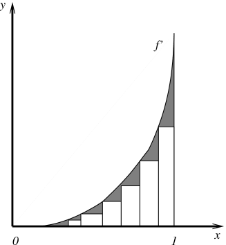
Figure 4: Interpretation of the collision rate in terms of Riemann integral.

This formula exactly says that we aim at approximating the integral of $f^{\prime}$ by a Riemann integral. In other words, if we are given $m-1=2^{k}-1$ real numbers $z_{1},\dots,z_{m-1}$ in $]0,1[$, with $0=z_{0}<z_{1}<\dots<z_{m-1}<z_{m}=1$, then the quantity

$$\rho=\sum_{i\in\{1,\dots,m\}}(z_{i}-z_{i-1})f^{\prime}(z_{i-1})$$

is the approximation of the integral of $f^{\prime}$ by a piece-wise constant function having $m$ steps. This fact is illustrated by figure 4. In this figure we draw the $f^{\prime}$ function, which integral between $0$ and $1$ exactly equals $1$ (since $f(1)-f(0)=1$). Points have been chosen to approximate this integral by a lower-bound piece-wise constant function. The rate of collision of our protocol will be exactly equal to the area in gray on the figure, which is also the approximation default. Therefore, if we have the best values of $z_{0},\dots,z_{m}$ for this integral, it is sufficient to set $y_{w}=z_{\#(w)}$, where $\#(w)$ is the numerical binary value that is represented by $w$. The reader can verify that this is obtained by setting:

$$p_{w}=\frac{z_{\#(w)2^{k-l(w)}+2^{k-l(w)}}-z_{\#(w)2^{k-l(w)}+2^{k-l(w)-1}}}{z_{\#(w)2^{k-l(w)}+2^{k-l(w)}}-z_{\#(w)2^{k-l(w)}}}.$$

Proposition 1

For all protocol of selection governed by a series of selective rounds as indicated in figure 2, we can associate a series of $m+1$ real numbers $z_{0},\dots,z_{m}$ in $[0,1]$, with $0=z_{0}<z_{1}<\dots<z_{m-1}<z_{m}=1$, such as the probability of success (non-collision) of the protocol is given by:

$$\rho=\sum_{i\in\{1,\dots,m\}}(z_{i}-z_{i-1})f^{\prime}(z_{i-1}).$$ (4)

In this case, the probabilities chosen to operate the different rounds of selection are given by:

$$p_{w}=\frac{z_{\#(w)2^{k-l(w)}+2^{k-l(w)}}-z_{\#(w)2^{k-l(w)}+2^{k-l(w)-1}}}{z_{\#(w)2^{k-l(w)}+2^{k-l(w)}}-z_{\#(w)2^{k-l(w)}}}.$$ (5)

Inversely, to all family of real numbers $z_{0},\dots,z_{m}$ verifying

$$0=z_{0}<z_{1}<\dots<z_{m-1}<z_{m}=1,$$

we can associate a protocol of selection whose probability of success and probabilities are given by equations (4) and (5).

So we are now left with the problem of finding optimal values for $z$. Analyzing a little further the value of $\rho$, we obtain the formula:

$$\begin{array}[]{lll}1-\rho&=&\displaystyle\int_{0}^{1}f^{\prime}(t)dt-\sum_{i\in\{1,\dots,m\}}(z_{i}-z_{i-1})f^{\prime}(z_{i-1})\\ &=&\displaystyle\sum_{i\in\{1,\dots,m\}}f(z_{i})-f(z_{i-1})-(z_{i}-z_{i-1})f^{\prime}(z_{i-1}).\end{array}$$

Three lemmas will allow us to analyze it.

Lemma 3

Let $\hbar$ be the piece-wise constant function defined by

$$\hbar:x\mapsto\frac{1}{m(z_{i}-z_{i-1})}\mbox{ for }x\in[z_{i-1};z_{i}[.$$ (6)

We have $\int^{0}_{1}\hbar(t)dt=1$ and

$$\begin{array}[]{l}\displaystyle\frac{1}{2m}\int_{0}^{1}\frac{f^{\prime\prime}(t)}{\hbar(t)}dt\\ =\displaystyle\sum_{i\in\{1,\dots,m\}}\int^{z_{i}}_{z_{i-1}}\frac{z_{i}-z_{i-1}}{2}f^{\prime\prime}(t)dt\\ =\displaystyle\sum_{i\in\{1,\dots,m\}}\frac{(z_{i}-z_{i-1})(f^{\prime}(z_{i})-f^{\prime}(z_{i-1}))}{2}.\end{array}$$

Moreover,

$$1-\rho-\frac{1}{2m}\int^{1}_{0}\frac{f^{\prime\prime}(t)}{\hbar(t)}dt\geq-\frac{1}{12}\sum_{i\in\{1,\dots,m\}}(z_{i}-z_{i-1})^{3}f^{\prime\prime\prime}(z_{i})$$

and

$$1-\rho-\frac{1}{2m}\int^{1}_{0}\frac{f^{\prime\prime}(t)}{\hbar(t)}dt\leq-\frac{1}{12}\sum_{i\in\{1,\dots,m\}}(z_{i}-z_{i-1})^{3}f^{\prime\prime\prime}(z_{i-1}).$$

Proof. 

$$\begin{array}[]{l}\displaystyle 1-\rho-\frac{1}{2m}\int^{1}_{0}\frac{f^{\prime\prime}(t)}{\hbar(t)}dt\\ \displaystyle=\sum_{i\in\{1,\dots,m\}}f(z_{i})-f(z_{i-1})-(z_{i}-z_{i-1})f^{\prime}(z_{i-1})\\ \qquad\qquad\qquad-\frac{(z_{i}-z_{i-1})(f^{\prime}(z_{i})-f^{\prime}(z_{i-1}))}{2}\\ \displaystyle=\sum_{i\in\{1,\dots,m\}}f(z_{i})-f(z_{i-1})\\ \qquad\qquad\qquad-(z_{i}-z_{i-1})\frac{f^{\prime}(z_{i})+f^{\prime}(z_{i-1})}{2}.\\ \end{array}$$

But $f$ is an harmonic function with positive coefficients, and radius of convergence from 0 at least 1, therefore:

$$\begin{array}[]{l}\displaystyle f(z_{i})=\sum_{j\geq 0}\frac{(z_{i}-z_{i-1})^{j}}{j!}f^{(j)}(z_{i-1})\\ \displaystyle f^{\prime}(z_{i})=\sum_{j\geq 1}\frac{(z_{i}-z_{i-1})^{j-1}}{(j-1)!}f^{(j)}(z_{i-1})\\ \end{array}$$

and we have

$$\begin{array}[]{l}f(z_{i})-f(z_{i-1})-\frac{z_{i}-z_{i-1}}{2}(f^{\prime}(z_{i})+f^{\prime}(z_{i-1}))\\ =(z_{i}-z_{i-1})^{3}{\displaystyle\sum_{j\geq 3}}(z_{i}-z_{i-1})^{j-3}\left[\frac{1}{j!}-\frac{1}{2(j-1)!}\right]\times\\ \qquad f^{(j)}(z_{i-1}),\\ =-(z_{i}-z_{i-1})^{3}{\displaystyle\sum_{j\geq 3}}(z_{i}-z_{i-1})^{j-3}\frac{1}{(j-1)!}\left[\frac{1}{2}-\frac{1}{j}\right]\times\\ \qquad f^{(j)}(z_{i-1}).\end{array}$$

We note that all the derivatives of $f$ are positive, and therefore all the term of this series are non-positive. Hence the second inequality. Moreover,

$$\begin{array}[]{l}\displaystyle\sum_{j\geq 3}(z_{i}-z_{i-1})^{j-3}\left[\frac{1}{2(j-1)!}-\frac{1}{j!}\right]f^{(j)}(z_{i-1})\\ \displaystyle\quad=\sum_{j\geq 3}(z_{i}-z_{i-1})^{j-3}\frac{j-2}{2(j!)}f^{(j)}(z_{i-1})\\ \displaystyle\quad\leq\sum_{j\geq 3}(z_{i}-z_{i-1})^{j-3}\frac{1}{12(j-3)!}f^{(j)}(z_{i-1})\\ \displaystyle\quad\leq\frac{1}{12}f^{\prime\prime\prime}(z_{i})\end{array}$$

$\square$

Lemma 4

Suppose $f^{\prime\prime}(0)>0$. Let the real numbers $z_{0},\dots,z_{m}$ in $[0,1]$, with $0=z_{0}<z_{1}<\dots<z_{m-1}<z_{m}=1$, that achieve the maximum value of $\rho=\sum_{i\in\{1,\dots,m\}}(z_{i}-z_{i-1})f^{\prime}(z_{i-1})$. Then we have:

$$\sum_{i\in\{1,\dots,m\}}(z_{i}-z_{i-1})^{2}\leq\frac{2}{mf^{\prime\prime}(0)},$$

and

$$\forall i\in\{1,\dots,m\}\quad z_{i}-z_{i-1}\leq\sqrt{\frac{2}{f^{\prime\prime}(0)}}\frac{1}{\sqrt{m}}.$$

Proof.  We have:

$$1-\rho=\sum_{i\in\{1,\dots,m\}}f(z_{i})-f(z_{i-1})-(z_{i}-z_{i-1})f^{\prime}(z_{i-1}),$$

and by Taylor expansion, there exists $b_{i-1}$ in the interval $]z_{i-1};z_{i}[$ such that

$$f(z_{i})-f(z_{i-1})=$$

$$(z_{i}-z_{i-1})f^{\prime}(z_{i-1})+\frac{(z_{i}-z_{i-1})^{2}}{2}f^{\prime\prime}(b_{i-1}).$$

Therefore $\displaystyle 1-\rho=\sum_{i\in\{1,\dots,m\}}\frac{(z_{i}-z_{i-1})^{2}}{2}f^{\prime\prime}(b_{i-1}).$

Since $\rho$ is a maximum value for all the choices of $z_{i}$, necessarily $1-\rho\leq 1/m$ (indeed, if we take $z_{i}=i/m$, we obtain a solution verifying $1-\rho\leq 1/m$). Therefore $z_{i}-z_{i-1}$ tends to $0$ when $m$ tends to infinity. The previous inequality taken term by term gives $z_{i}-z_{i-1}\leq\sqrt{\frac{2}{f^{\prime\prime}(0)}}\frac{1}{\sqrt{m}}$, and since all the $f^{\prime\prime}(b_{i})$ are bounded below by $f^{\prime\prime}(0)$, we obtain

$$\sum_{i\in\{1,\dots,m\}}(z_{i}-z_{i-1})^{2}\leq\frac{2}{mf^{\prime\prime}(0)}.$$

$\square$

Lemma 5

If $f^{\prime\prime}$ is piece-wise continuous, the minimum of the value $\int_{0}^{1}\frac{f^{\prime\prime}(t)}{h(t)}dt$ on the functions $h$ piece-wise continuous and verifying $\int_{0}^{1}h(t)dt=1$ is obtained by $h^{*}:x\mapsto\frac{\sqrt{f^{\prime\prime}(x)}}{\int_{0}^{1}\sqrt{f^{\prime\prime}(t)}dt}$ and therefore equals $\left(\int_{0}^{1}\sqrt{f^{\prime\prime}(t)}dt\right)^{2}$.

The proof of lemma 5 is easily obtained if $f^{\prime\prime}$ is a piecewise constant-function, and we use uniform convergence of piecewise constant-functions to piece-wise continuous functions.

Proposition 2

If $f^{\prime\prime}(0)>0$, whatever the series of $m$ values of $z_{.}$ used, we have:

$$1-\rho\geq\frac{\left(\int_{0}^{1}\sqrt{f^{\prime\prime}(t)}dt\right)^{2}}{2m}-\frac{f^{\prime\prime}(1)}{3\sqrt{2}f^{\prime\prime}(0)^{3/2}}\frac{1}{m^{3/2}}.$$

Proof.  By lemma (3) we have:

$$1-\rho\geq\frac{1}{2m}\int^{1}_{0}\frac{f^{\prime\prime}(t)}{\hbar(t)}dt-\frac{1}{12}\sum_{i\in\{1,\dots,m\}}(z_{i}-z_{i-1})^{3}f^{\prime\prime\prime}(z_{i}).$$

Then applying lemma (5) for $\hbar=h$ gives

$$1-\rho\geq\frac{1}{2m}\int^{1}_{0}\frac{f^{\prime\prime}(t)}{\hbar(t)}dt-\frac{1}{12}\sum_{i\in\{1,\dots,m\}}(z_{i}-z_{i-1})^{3}f^{\prime\prime\prime}(z_{i}).$$

Then the second inequality of lemma (4) gives:

$$\begin{array}[]{l}\displaystyle 1-\rho\geq\frac{1}{2m}\int^{1}_{0}\frac{f^{\prime\prime}(t)}{\hbar(t)}dt\\ \qquad\displaystyle-\frac{1}{12\sqrt{m}}\sqrt{\frac{2}{f^{\prime\prime}(0)}}\sum_{i\in\{1,\dots,m\}}(z_{i}-z_{i-1})^{2}f^{\prime\prime\prime}(z_{i}).\end{array}$$

Since $f^{\prime\prime\prime}(z_{i})\leq f^{\prime\prime\prime}(0)$, it gives:

$$\begin{array}[]{l}\displaystyle 1-\rho\geq\frac{1}{2m}\int^{1}_{0}\frac{f^{\prime\prime}(t)}{\hbar(t)}dt\\ \qquad\displaystyle-\frac{f^{\prime\prime\prime}(0)}{12\sqrt{m}}\sqrt{\frac{2}{f^{\prime\prime}(0)}}\sum_{i\in\{1,\dots,m\}}(z_{i}-z_{i-1})^{2}.\end{array}$$

Finally the first inequality of lemma (4) gives:

$$1-\rho\geq\frac{1}{2m}\int^{1}_{0}\frac{f^{\prime\prime}(t)}{\hbar(t)}dt-\frac{f^{\prime\prime\prime}(0)}{12\sqrt{m}}\sqrt{\frac{2}{f^{\prime\prime}(0)}}\frac{2}{mf^{\prime\prime}(0)}.$$

Hence the result. $\square$

This result clearly shows what is the maximum efficiency of the protocol whatever the chosen values of probabilities, and therefore the maximum we can asymptotically expect, that is

$$1-\rho\approx\frac{\left(\int_{0}^{1}\sqrt{f^{\prime\prime}(t)}dt\right)^{2}}{2m}.$$

The strategy of approaching $h$ by a piecewise constant-function therefore gives a result asymptotically optimal.

We note also that as the number of round increases, the collision rates systematically decreases, and this factor of division converges to 2 as the number of rounds increases. It means that we can reduce the collision rate by an arbitrary low level by using a reasonably small number of additional rounds. For applications that suffer from retransmissions (and jitter) this property can have a considerable impact.

However, further experiments showed, that in the 802.11b framework where the jitter was not important and the throughput was to be optimized, the good number of mini-slots to use was 6.

Some more results on the approximation of a function by Riemann integrals are worth to be noted. We are interested in the following problem:

Problem 1

Let $\varphi$ a non-decreasing function from $[0;1]$ to $[0;1]$, with $\varphi(0)=0$ and $\varphi(1)=1$. We are looking for a piecewise constant function $\psi$, with $m+1$ pieces, such that

$$\left\{\begin{array}[]{l}\forall z\in[0;1]\quad\psi(z)\leq\varphi(z),\\ \displaystyle\int_{0}^{1}\left(\varphi(z)-\psi(z)\right)dz\mbox{ is minimum}.\end{array}\right.$$

Clearly, this problem is the optimization formulation of the preceding issue when, for $z\in[0;1]$, $\varphi(z)=f^{\prime}(z)/f^{\prime}(1)$.

Proposition 3

If $z\mapsto z\varphi(z)$ is convex, $m=1$, and $\varphi$ continuously derivable, then the minimum for $g$ is reached with a step $z$ verifying $(1-z)\varphi^{\prime}(z)=\varphi(z)$.

Proof.  If the step is $z\in[0,1]$, then

$$\int_{0}^{1}(\varphi(t)-\psi(t))dt=\int_{0}^{1}\varphi(t)dt-(1-z)\varphi(z).$$

Note that necessarily there is some $z^{*}\in]0;1[$ such that $\varphi(z^{*})>0$ and this particular $z^{*}$ does better than $z=0$ or $z=1$. The best $z$ necessarily then verifies $\frac{d}{dz}(1-z)\varphi(z)=0$. $\square$

Proposition 4

For a fixed $m$, for any $\varphi$ function, there is a $\psi$ function that reaches the minimum. This minimum will be noted $c_{m}$.

Proof. L Set

$$c_{m}=\inf_{\mbox{\begin{tabular}[]{l}$\psi$ piece wise constant\\ with $m+1$ pieces,\\ and $\psi\leq\varphi$\end{tabular}}}(\varphi(t)-\psi(t))dt.$$

Let $\psi_{p}$ be a series of piece-wise constant functions, with $m+1$ pieces, such that

$$\lim_{p\rightarrow\infty}\int_{O}^{1}(\varphi(t)-\psi_{p}(t))dt=c_{m}.$$

Let $z^{(1)}_{p}\leq\dots\leq z^{(m)}_{p}$ be the points where $g_{p}$ is not continuous. Since $[0;1]$ is compact, let us extract a converging series $z^{(1)}_{\sigma_{1}(p)}$ (that is, $\sigma_{1}$ is an increasing function from IN to IN such that the series $z^{(1)}_{\sigma_{1}(p)}$, $p\in\hbox{\rm I$\mskip-3.0mu$N\/}$ is converging), and $\sigma_{2}$ such that $z^{(2)}_{\sigma_{2}(\sigma_{1}(p))}$ is converging, and so on to $\sigma_{m}$ such that $z^{(m)}_{\sigma_{m}o\dots o\sigma_{1}(p)}$ is converging. Setting $\sigma=\sigma_{m}o\dots o\sigma_{1}$ we have that $\sigma$ is increasing from IN to IN and for each $i\in\{1,\dots,m\}$, $z^{(i)}_{\sigma(p)}$, $p\in\hbox{\rm I$\mskip-3.0mu$N\/}$ is converging.

Let us then note $z^{(i)}_{*}=\lim_{p\rightarrow\infty}z^{(i)}_{\sigma(p)}$, for $i\in\{1,\dots,m\}$, $z^{(0)}_{*}=0$, $z^{(m+1)}_{*}=1$, and $\psi^{*}$ such that for $i\in\{1,\dots,m+1\}$, and $z\in[z^{(i-1)}_{*},z^{(i)}_{*}[$, $\psi^{*}(z)=\varphi(z^{(i-1)}_{*})$.

Let $\varepsilon>0$ be a real number. There is a $\eta>0$ such that for all $i\in\{1,\dots,m\}$, $|z-z^{(i)}_{*}|<\eta$ implies $|\varphi(z)-\varphi(z^{(i)}_{*})|<\varepsilon$. If $\eta>\varepsilon$, set $\eta=\varepsilon$. Then there is a $P\in\hbox{\rm I$\mskip-3.0mu$N\/}$ such that $p\geq P$ implies $|z^{(i)}_{*}-z^{(i)}_{\sigma(p)}|\leq\eta$.

We see that for each $i\in\{1,\dots,m\}$,

$$\psi_{*}(z^{(i)}_{*})=\varphi(z^{(i)}_{*})\geq\varphi(z^{(i)}_{p})-\varepsilon=\psi_{p}(z^{(i)}_{p})-\varepsilon$$

for $p\geq P$, and therefore

$$\int_{0}^{1}\left(\psi_{*}(t)-\psi_{p}(t)\right)dt\geq-\varepsilon-m\eta\geq-(m+1)\varepsilon.$$

This is true for all $\varepsilon>0$, and so $\int_{0}^{1}\psi_{*}(t)dt\geq c_{m}.$ $\square$

Proposition 5

Let $A$ the function from $\hbox{\rm I$\mskip-3.0mu$R\/}^{m}$ to IR given by

$$A(z_{1},\dots,z_{m})=$$

$$\sum_{i=2}^{i=m}(z_{i}-z_{i-1})\varphi(z_{i-1})+(1-z_{m})\varphi(z_{m}).$$

Then

$$\max_{(z_{1},\dots,z_{m})\in[0;1]^{m}}A(z_{1},\dots,z_{m})=c_{m}.$$

Proof.  It suffices to show that for the maximum we have $z_{1}\leq\dots\leq z_{m}$. Note that if $\alpha<\beta$, then

$$(\beta-\alpha)\varphi(\alpha)+(1-\beta)\varphi(\beta)>(\alpha-\beta)\varphi(\beta)+(1-\alpha)\varphi(\alpha).$$

It follows that

$$A(z_{1},\dots,z_{i-1},\alpha,\beta,z_{i+1},\dots,z_{m})\geq$$

$$A(z_{1},\dots,z_{i-1},\beta,\alpha,z_{i+1},\dots,z_{m}).$$

Therefore, ordering the arguments of $A$ maximizes its results (use for instance bubble sort). $\square$

Those results open tools for promising optimization.

3 Practical implementation

Figure 5: Strategies of optimization of the values of $p$

In figure 5, we show the basic principles of an optimization based on our mathematical analysis. A preliminary step consists in fixing a scenario, that is the probabilities that a given number of stations appears. For instance we set as previously

$$P[\mbox{Number of emitting stations}=n]=q_{n}.$$

And we consider

$$f(x)=\sum_{n\geq 1}q_{n}x^{n}.$$

Then we have an $\hat{h}$ function defined by $\hat{h}(x)=\sqrt{f^{\prime\prime}(x)}$ ($\hat{h}$ is the equivalent of $h^{*}$ in the previous section, but without the normalization $\int_{0}^{1}h^{*}(t)dt=1$). And we take a number $M$ largely greater than $m=2^{k}$ and we compute $H$ as follows

$$\left\{\begin{array}[]{l}H(0)=0\\ H(i+1)=H(i)+\hat{h}\left(\frac{i+1/2}{M}\right)\\ \qquad\mbox{ for }i\in\{0,\dots,M-1\}\\ \end{array}\right.$$

and we define $z_{j}$ for $j\in\{0,\dots,m\}$ by

$$\left\{\begin{array}[]{l}z_{0}=0,\\ z_{j}=\frac{1}{M}\min\left\{i:\frac{H(i)}{H(M)}\geq\frac{j}{m}\right\}\\ \qquad\mbox{ for }j\in\{1,\dots,m-1\},\\ z_{m}=1.\end{array}\right.$$

Finally we set

$$p_{w}=\frac{z_{\#(w)2^{k-l(w)}+2^{k-l(w)-1}}-z_{\#(w)2^{k-l(w)}+2^{k-l(w)}}}{z_{\#(w)2^{k-l(w)}}-z_{\#(w)2^{k-l(w)}+2^{k-l(w)}}}$$

where $w$ is a word in the $\{0,1\}$ alphabet, $\#(w)$ represents the numerical binary value denoted by $w$ and $l(w)$ the length of the word $w$.

4 Numerical results

In the first part of this section, we compare the collision rate of our method to that of CONTI [3]. We show that for some parameter our collision rate is always favorable, and therefore systematically results in a better performance to CONTI. Along with the native 802.11b protocol [1], we compare to two high performing protocols, the Idle Sense one [12] and the additive congestion window increase /decrease protocol [11]. Finally we concentrate on fairness issues for these different schemes, based on the Jain index [13].

4.1 A tuning of the probabilities

$l(w)$ 0 1 2 3 4 5 $p_{w}$ 0.07 0.2 0.25 0.33 0.4 0.5

Table 1: Values taken by CONTI.

Figure 6: Various collision rates obtained with our algorithm compared to CONTI.

An essential step is to set the values of $q_{n}$. One idea is to set a favorite interval of operation, say $\{2,\dots,N\}$, and fix, for $n\in\{2,\dots,N\}$, and some $\alpha\in[0,1]$,

$$q_{n}=\frac{n^{-\alpha}}{\sum_{i=2}^{i=N}i^{-\alpha}}.$$ (7)

This distribution allows to take into account in a balanced way loaded or non loaded networks. In figure 6, we show different probability curves obtained for $N=100$, and various values of $\alpha$.

In order to see the advantage of our optimization techniques, we compare our results to that performed by CONTI [3]. In our context, one can simply view CONTI as a special assignment of the values of $p_{w}$ that only depends on the length $w$. For completeness, we recall the values taken in table 1.

Globally, we can see that these functions perform remarkably well compared to CONTI. Whereas the latter has a collision rate between 4.5 and 6.5%, with a maximum for the 4.5% rate, our algorithms fall often under 4%. The value $\alpha=0$ allows to give equal weights to all the events. In practice, we see that this global optimization tends to pay more attention to the cases where more stations are present (50 to 100) at the expense of more collisions when two to five stations are present in the system. On the contrary $\alpha=1$ performs well when a small number of stations are present at the expense of lesser performance over 60 stations. A good compromise seems to be $\alpha=0.7$ which varies between 3.9% and 6.3% with an average improvement to CONTI of 13.9% in collision rate. For the cases $\alpha=0$ and $\alpha=0.5$, the improvement - although in some cases negative - is on average even better, respectively 21.1% and 17.8%. In the following we will set $\alpha=0.7.$ For sake of completeness, we give in figure 2 our probability values so that the reader can replicate our experiments without further considerations on choosing $\alpha$.

4.2 Comparative bandwidth

$$\begin{array}[]{|ll|ll|}\hline\cr&&p_{00000}&0.470679\\ p&0.0628357&p_{00001}&0.471427\\ p_{0}&0.166808&p_{00010}&0.472147\\ p_{1}&0.305488&p_{00011}&0.472882\\ p_{00}&0.295586&p_{00100}&0.473527\\ p_{01}&0.328258&p_{00101}&0.474214\\ p_{10}&0.375175&p_{00110}&0.474668\\ p_{11}&0.423688&p_{00111}&0.475313\\ p_{000}&0.388521&p_{01000}&0.476041\\ p_{001}&0.398651&p_{01001}&0.476681\\ p_{010}&0.407585&p_{01010}&0.477124\\ p_{011}&0.416295&p_{01011}&0.477647\\ p_{100}&0.429211&p_{01100}&0.477976\\ p_{101}&0.444548&p_{01101}&0.478795\\ p_{110}&0.457931&p_{01110}&0.478203\\ p_{111}&0.465291&p_{01111}&0.48056\\ p_{0000}&0.442201&p_{10000}&0.479927\\ p_{0001}&0.444984&p_{10001}&0.480932\\ p_{0010}&0.447669&p_{10010}&0.481663\\ p_{0011}&0.450083&p_{10011}&0.48324\\ p_{0100}&0.452293&p_{10100}&0.484177\\ p_{0101}&0.454545&p_{10101}&0.485714\\ p_{0110}&0.456444&p_{10110}&0.486056\\ p_{0111}&0.459286&p_{10111}&0.486726\\ p_{1000}&0.462745&p_{11000}&0.490291\\ p_{1001}&0.466754&p_{11001}&0.491979\\ p_{1010}&0.469799&p_{11010}&0.491329\\ p_{1011}&0.473795&p_{11011}&0.490566\\ p_{1100}&0.475827&p_{11100}&0.489796\\ p_{1101}&0.478916&p_{11101}&0.492754\\ p_{1110}&0.484211&p_{11110}&0.492188\\ p_{1111}&0.483871&p_{11111}&0.491667\\ \hline\cr\end{array}$$

Table 2: Values obtained for the $p_{\cdot}$’s for $\alpha=0.7$ and $N=100$.

Figure 7: Comparative total throughput for different protocols.

We set the general parameters as follows, according to the IEEE 802.11b norm. The SIFS and DIFS times are set to $10\mu s$ and $50\mu s$ respectively. The time-slot interval for CRP is set to $20\mu s$. The size of the payload of a packet is set to 1500 bytes. A packet (either regular or ACK) contains a physical header of $96\mu s$. On top of that, the MAC head and tail represent in all 19 bytes in a regular packet, and 14 bytes in an ACK one, that are transmitted at the maximum speed, that is 11Mbit/s. We now further describe the specificity of each protocol.

• The 802.11b norm [1]. Each station has a $CW$ parameter. At the beginning, a station chooses a $\kappa$ - called back-off counter - randomly in the interval $\{0,\dots,CW-1\}$. If $\kappa=0$, the transmission begins immediately. Otherwise, if an empty time-slot is observed, $\kappa$ is decreased by one. At the end of a transmission, the value of $CW$ itself is updated to $CWMin$ if the transmission was successful, and to $\min(CWMax,2*CW)$ if a collision occurred. We have set as in the norm $CWMin=32$ and $CWMax=1024$.

• The Idle Sense method [12]. At the end of a transmission, successful or not, the terminal stores the number of idle time-slots before its transmission. After 5 transmissions, the terminal computes the average waited time-slots. If this number is inferior to $5.68$, the congestion window is updated by

  $$CW=\min(CWMax,CW*1.2).$$

  Otherwise, the new $CW$ is given by:

  $$CW=\max(CWMin,2*CW/(2+1e-3*CW)).$$

• The additive congestion window increase/decrease [11]. At the end of an unsuccessful transmission, $CW$ is set to $\min(CWmax,CW+32)$. If the transmission is successful, the station flips a biased coin, and with probability $0.1809$ updates $CW$ by

  $$CW:=\max(CWmin,CW-32)$$

  and otherwise does not change $CW$.

• The CONTI method [3]. At each step a CRP of six time-slots is applied with the probabilities given by table 1. The surviving stations transmit.

• Our method - MAC in fixed congestion window. We apply a CRP of six time-slots. We have used the probabilities of table 2.

Our results are presented in figure 7. In this figure, we plot for various numbers of stations the total throughput observed in the system. We clearly see that all the proposed methods improve significantly the original IEEE 802.11b mechanism. The methods based on adaptive tuning of the congestion window, namely [12, 11], achieve quite close performances. The CONTI method performs very well. Our method gives the best performance in all cases, and has a total improvement as far as 31.4% for 100 stations to the original norm.

4.3 Fairness considerations

Figure 8: Comparative Jain index for different protocols.

In this part we take into consideration the fairness issues. For each of the experiments, we have observed a series of 10000 successful transmission, and assigned to each station $i$ the number $x_{i}$ of packets it managed to transmit. In order to evaluate the fairness, we use the Jain index [13], defined by:

$$Index=\frac{\left(\sum x_{i}\right)^{2}}{n\sum x_{i}^{2}}.$$

This index is always between $0$ and $1$, and closer to $1$ if the system is more fair. Our results are given in figure 8. Note that our method is equivalent to the CONTI method from the fairness point of view. The results plotted are averages obtained after a series of 10 tests.

The results show different behaviors. We observe as in [12] that slow congestion window methods tend to generate some unfairness. We also notice that new method hardly improve the quality of the original IEEE 802.11b norm. Note, anyway, that our method achieves the best fairness performance.

5 Conclusion

In this paper we have demonstrated the efficiency of MAC protocols with constant congestion window size in the wireless context. We have determined their limits in terms of avoidance of collision, and shown that they perform very well in terms of fairness. The tuning that we propose achieves the best throughput performance in the 802.11b framework to our knowledge. This advocate for a more extensive use of these methods, and the building of devices including this new access control mode. This is not necessarily a simple task, since the proposed scheme is not compatible with the previous ones excepted CONTI, but is a promising way to achieve better wireless networks.

$k$ Number of rounds of selection. $m$ $2^{k}$. $r(t)$ Try-bit at the $t^{\mbox{th}}$ round of selection, $t\in\{1,\dots,k\}$. $R(t)$ Local try-bit (at a station) at the $t^{\mbox{th}}$ round of selection, $t\in\{1,\dots,k\}$. $q_{n}$ Probability that $n$ station try to emit. $w$ Word in the alphabet $\{0,1\}$. $l(w)$ Length of the word $w$. $\#(w)$ Binary value represented by $w$ $p$ Probability that a station emits a signal at the first round of selection. $p_{w}$ Probability that a non-eliminated station emits a signal at the round $l(w)+1$, given that the preceding try-bits where $r(1),\dots,r(l(w))=w$. $f$ Generating function of $q_{.}$, see equation (1). $f_{w}$ Generating function of the number of non-eliminated stations, in the event $w$. $g$ Generating function of the number of non-eliminated stations after $k$ rounds. $\rho$ Success rate (as opposed to the collision rate). $\delta_{w}$ Local step, see equation (2). $y_{w}$ Cumulative step, see equation (3). $z_{i}$ Riemann steps for $f^{\prime}$ in $[0,1]$, $i\in\{0,\dots,m\}$. $\varphi$ Continuous function in $[0;1]$ to be approximated. $\psi$ Piece-wise constant function that approximate $\varphi$. $c_{m}$ Best approximation gap for the approximation of $\varphi$ with $m$ pieces. $\sigma$ Increasing function from IN to IN that emphasizes extraction. $A$ Function of $\hbox{\rm I$\mskip-3.0mu$R\/}^{m+1}$ to IR that reaches approximation for $\varphi$. $\hbar$ Density step function defined after $z_{\cdot}$, see equation (6). $h^{*}$ Density function that minimizes $\int_{0}^{1}f^{\prime\prime}(t)/h(t)dt$, see proposition 2. $\hat{h}$ Density function taken for the algorithmic choices of $z_{\cdot}$, $\hat{h}(x)=\sqrt{f^{\prime\prime}(x)}$. $M$ Large number compared to $m$. $N$ Maximum number of foreseen stations. $\alpha$ Parameter to set the values of $q_{\cdot}$, see equation (7). $x_{i}$ In the experiments, amount of packets that an individual station has emitted.

Table 3: Notations used in this paper.

References

• [1] Higher-speed physical layer extension in the 2.4 GHz band. IEEE Std 802.11b-1999 Part 11: wireless LAN medium access control (MAC) and physical layer (PHY) specifications.
• [2] IEEE standard for local and metropolitean network. Part 16: Air Interface for Broadband Wireless Access System (IEEE802.16 REVd D5-2004), May 2004.
• [3] Z. Abichar and M. Chang. CONTI: constant-time contention resolution for WLAN access. In Proceedings of Networking, number LNCS 3462, pages 358–369, 2005.
• [4] S. Beuerman and E. Coyle. The delay characteristics of CSMA/CD networks. IEEE Transactions on Communications, 36(5):553–563, May 1988.
• [5] G. Bianchi. Performance analysis of the IEEE 802.11 distributed coordination function. IEEE Journal on Selected Areas in Communications, 18(8):535–547, March 2000.
• [6] L. Bononi, M. Conti, and E. Gregory. Optimization of IEEE 802.11 wireless LANs performance. IEEE Transactions of Parallel and Distributed Systems, 15(1):66–80, January 2004.
• [7] F. Cali, M. Conti, and E. Gregori. Dynamic tuning of the IEEE 802.11 protocol to achieve a theoretical throughput limit. IEEE/ACM Transactions on Networking, 8(6):783–799, December 2000.
• [8] J. Capetanakis. Generalized TDMA: the multi-accessing tree protocol. IEEE Transactions on Communications, COM-27(10):1476–1484, Oct. 1979.
• [9] J. Capetanakis. Tree algorithms for packet broadcast channels. IEEE Transactions on Information Theory, IT-25(5):505–515, Sept 1979.
• [10] G. Fayolle, P. Flageolet, M. Hofri, and P. Jacquet. Analysis of a stack algorithm for random multiple-access communication. IEEE Transactions on Information Theory, IT-31(2):244–254, March 1985.
• [11] J. Galtier. Optimizing the IEEE 802.11b performance using slow congestion window decrease. In Proccedings of the 16th ITC Specialist Seminar on performance evaluation of wireless and mobile systems, pages 165–176, Antwerpen, August/Sept 2004.
• [12] M. Heuse, F. Rousseau, R. Guillier, and A. Duda. Idle sense: An optimal access method for high throughput and fairness in rate diverse wireless LANs. In Proceedings of SIGCOMM 05, Philadelphia, USA, August 2005.
• [13] R. Jain, D.-M. Chiu, and W. Hawe. A quantitative measure of fairness and discrimination for ressource allocation in shared computer system. Technical Report DEC-TR-301, Digital Equipment Corporation, 1984.
• [14] K. Jamieson, H. Balakrishnan, and Y. Tay. Sift: A MAC protocol for event-driven wireless sensor networks. Technical Report 894, MIT Laboratory for Computer Science, May 2003.
• [15] A. Janssen and M. de Jong. Analysis of contention tree algorithms. IEEE Transactions on Information Theory, 46(6):2163–2172, Sept 2000.
• [16] L. Kleinrock and F. Tobagi. Packet switching in radio channels: Part I - carrier sense multiple access modes and their throughput-delay characteristics. IEEE Transactions on Communications, 23(12):1400–1416, December 1975.
• [17] J.-B. Seo, H.-W. Lee, and C.-H. Cho. Performance of IEEE 802.16 random access protocol - steady state queuing analysis. In Proceedings of Globecom, number WLC17-2, November 2006.
• [18] European Telecommunication Standard. HIgh PErformance Radio Local Area Network (HIPERLAN) Type 1; Functional Specification, 1996.
• [19] B. Tsybakov and A. Mikhailov. Free synchronous packet access in a broadcast channel with feedback. Prob. Inform. Trans., 14:259–280, Oct.-Dec. 1978.
• [20] H. Wu, Y. Peng, K. Long, S. Cheng, and J. Ma. Performance of reliable transport protocol over IEEE 802.11 wireless LAN: analysis and enhancement. In Proceedings of INFOCOM’02, 2002.
• [21] Y. Xiao. Saturation performance metrics of the IEEE 802.11 MAC. In Proc. of The IEEE Vehicular Technology Conference (IEEE VTC 2003 Fall), pages 1453–1457, Orlando, Florida, USA, Oct 2003.