Integrability, stability, and adiabaticity in nonlinear stimulated Raman adiabatic passage.

Abstract

We study dynamics of a two-color photoassociation of atoms into diatomic molecules via nonlinear Stimulated Raman adiabatic passage (STIRAP) process. This system has a famous counterpart in (linear) quantum mechanics, and been discussed recently in the context of generalizing quantum adiabatic theorem to nonlinear systems. Here we use another approach to study adiabaticity and stability in the system: we apply methods of classical Hamiltonian dynamics. We found nonlinear dynamical instabilities, cases of complete integrability, and improved conditions of adiabaticity.

Adiabatic theorem Sanders of quantum mechanics has found wide applications in quantum state manipulations. Dynamics of Bose-Einstein condensates (BEC) GP introduces paradigm of nonlinearity into a quantum world (note studies on nonlinear Landau-Zener models Zobay ; IW , solitons, shock waves, etc). Along with nonlinearity, it also brings a question of how to analyze adiabaticity in nonlinear systems. It is not justified to apply the adiabatic condition of quantum mechanics to nonlinear BEC systems Pu ; Reinhardt . Instead, a general method was recently suggested Pu and applied to a specific example of two-color Raman photoassociation system Javanainen . Here, we consider the same example as in Pu ; Javanainen and notice that, as a typical nonlinear system, it possesses many counterintuitive difficulties in the analysis. The goal of our paper is twofold. Firstly, we (inspired by ideas of Pu ) suggest another approach to analyze adiabaticity and stability in nonlinear BEC-related systems: we use methods of classical Hamiltonian dynamics AKN . Secondly, we improve a theory of nonlinear STIRAP (Stimulated Raman adiabatic passage).

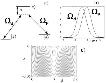
Figure 1: (a) A three-level $\Lambda$-system (b) Counterintuitive STIRAP sequence of pulses $\Omega_{p,d}$ (c) Phase portrait of (3). As parameters are changing in accordance with a pulse sequence shown in (b), the stable fixed point (corresponding to the dark state) moves from $z=0$.

Following Pu ; Javanainen , consider a three-level $\Lambda$-system shown in Fig. 1a. The state $|a\rangle$ corresponds to an atomic BEC, which is coupled to an excited diatomic molecular BEC (the state $|e\rangle$) via a Raman laser pulse $\Omega_{p}$ (”pump”). A single-photon detuning $\Delta$ is the difference between a frequency of the pump laser and the frequency of transition between $|a\rangle$ and $|e\rangle$. The state $|e\rangle$ is, in turn, coupled to the ground state of the molecular BEC by a laser pulse $\Omega_{d}$ (”dump”). In other words, a pair of atoms from $|a\rangle$ is photoassociated by a pump field of molecular Rabi frequency $\Omega_{p}$ into a molecule in the excited state $|e\rangle$, which is subsequently driven into the ground molecular state. This system is intrinsically nonlinear, as it involves merging of atoms into diatomic molecules. Its linear counterpart is widely used in quantum manipulations: STIRAP STIRAP is well-established technique for transferring population from $|a\rangle$ to $|g\rangle$ in three-level quantum systems. The gist of the technique is as following. Intuitively, one may think of transferring firstly the population from $|a\rangle$ to $|e\rangle$ by means of $\Omega_{p}$ pulse, and then from $|e\rangle$ to $|g\rangle$. However, the state $|e\rangle$ often suffers from spontaneous emission. STIRAP counterintuitive sequence of pulses STIRAP consists of overlapping $\Omega_{p,d}$ pulses, with $\Omega_{d}$ going first (see Fig. 1b). STIRAP process in both linear and nonlinear ${\Lambda}$-systems is based on the existence of a dark state which is a superposition of only $|a\rangle$ and $|g\rangle$ states (and therefore almost does not suffer from spontaneous emission of light, which explains the notation; another notation for the dark state is coherent population trapping (CPT) state Pu ). An instantaneous dark state is determined by values of $\Omega_{p,d}$; population transfer happens via the dark state as $\Omega_{p,d}$ are slowly changed, with $|e\rangle$ state remaining almost unpopulated. Stability and adiabaticity of the system in the dark state is essential for efficiency of population transfer. In contrast to its linear counterpart, the theory of nonlinear STIRAP is not well developed yet. This process is very important for BEC physics, as it allows to achieve BEC of molecules Winkler . Mean-field approach has shown to be reliable in such systems Mackie ; Javanainen ; Pu . Neglecting mean-field collisional interactions and spontaneous emission, the mean-field equations are Pu

$$i\dot{\psi}_{a} = \Omega_{p}\psi_{a}^{*}\psi_{e},\quad i\dot{\psi}_{g}=\frac{\Omega_{d}}{2}\psi_{e},$$

$$i\dot{\psi}_{e} = \Delta\psi_{e}+\frac{\Omega_{p}}{2}\psi_{a}^{2}+\frac{\Omega_{d}}{2}\psi_{g},$$ (1)

where amplitudes $\psi_{a,e,g}$ are normalized as $|\psi_{a}|^{2}+2(|\psi_{g}|^{2}+|\psi_{e}|^{2})=1$. The dark state vector is given by (up to a phase factor) ${\bf\Psi}_{0}=(\psi_{a}^{0},\psi_{e}^{0},\psi_{g}^{0})^{T}$, where $\psi_{a}^{0}=\Bigl{[}\frac{2\Omega_{d}}{\Omega_{d}+\Omega_{e}}\Bigr{]}^{1/2},\psi_{e}^{0}=0,\psi_{g}^{0}=-\frac{2\Omega_{p}}{\Omega_{d}+\Omega_{e}},$ with $\Omega_{e}=\sqrt{\Omega_{d}^{2}+8\Omega_{p}^{2}}$. Linearization about the dark state Pu gives a dynamical system with three eigenfrequencies: $\omega_{0}=0,\quad\omega_{\pm}=\frac{1}{2}[\Delta\pm(\Delta^{2}+\Omega_{d}\Omega_{e})^{1/2}].$ The frequencies $\omega_{0,\pm}$ are all real. However, it does not guarantee that the system is always dynamically stable: there might be nonlinear instabilities.

We recast the model into the form of a two-degree-of-freedom (2 d.o.f.) classical Hamiltonian system, and use the classical adiabatic theory and the resonance normal forms theory available in AKN ; Duist . Eqs. (1) are equivalent to Hamiltonian equations of motion of the effective classical Hamiltonian

$$H=\Omega_{p}\left[x_{2}\frac{y_{1}^{2}-x_{1}^{2}}{2}-x_{1}y_{2}y_{1}\right]-\frac{\Omega_{d}}{2}(x_{2}x_{3}+y_{2}y_{3})-\Delta\frac{x_{2}^{2}+y_{2}^{2}}{2}.$$ (2)

Here $x_{k}$ are canonical momenta, while $y_{k}$ are the coordinates, being related to the old ”variables” (complex numbers $\psi_{i}$) as $\psi_{a}=x_{1}+iy_{1},\quad\psi_{e}=x_{2}+iy_{2},\quad\psi_{g}=x_{3}+iy_{3}.$ The system has two degrees of freedom only: there exists integral of motion $N=x_{1}^{2}+y_{1}^{2}+2(x_{2}^{2}+y_{2}^{2}+x_{3}^{2}+y_{3}^{2})=1$.

Firstly, we consider the case $\Delta=0$ (single-photon resonance). Let $H=0$. On this manifold, dynamics at constant parameters $\Omega_{p,d}$ is completely integrable. Indeed, $I_{2}\equiv x_{2}/y_{2}$ is the additional integral of motion. As a result, $I_{3}\equiv I_{2}x_{3}+y_{3}$ and $I_{1}\equiv I_{2}\frac{y_{1}^{2}-x_{1}^{2}}{2}-x_{1}y_{1}$ are also integrals of motion. Integrability of the system with $\Delta=0$ at $H=0$ energy manifold is an important finding of this paper. In case $\Omega_{p,d}$ are changing with time, the system may leave the $H=0$ energy manifold. However, in case initial conditions are such that $I_{1,3}=0$, then even with time-dependent parameters dynamics will be confined to the initial $H=0$ manifold. The particular case considered in Pu (where all population is initially in $|a\rangle$) is of this type. Indeed, initially $x_{2,3}=y_{2,3}=0$ (therefore, $H=0$). As parameters are changed, $I_{1},I_{3}$ and $H$ all remain equal to zero, see Fig. 2, where the example of Pu is presented. The pulses are $\Omega_{p,d}=\Omega_{0}e^{-(t-t_{p,d})^{2}},$ with $t_{d}<t_{p}$. With $H=\mbox{const}\equiv 0$, we can reduce the system to a $1\frac{1}{2}$ d.o.f. classical Hamiltonian. Without loss of generality, let $I_{2}=0$. Therefore, only $x_{1},x_{3},y_{2}$ are non-zero during the evolution. The equations of motion are $\dot{x_{1}}=\Omega_{p}x_{1}y_{2},\quad\dot{x_{3}}=\frac{\Omega_{d}}{2}y_{2},\quad\dot{y_{2}}=-\frac{\Omega_{d}}{2}x_{3}-\frac{\Omega_{p}}{2}x_{1}^{2}.$ Introducing new variables $\phi$ and $z$ as $x_{3}=\frac{1}{\sqrt{2}}\sqrt{1-x_{1}^{2}}\cos\phi,\quad y_{2}=\frac{1}{\sqrt{2}}\sqrt{1-x_{1}^{2}}\sin\phi,\quad x_{1}=\exp[z],$ the equations of motion correspond now to the classical Hamiltonian

$${\cal H}=-\frac{\Omega_{d}}{2}z+\frac{\Omega_{p}}{\sqrt{2}}\sqrt{1-e^{2z}}\cos\phi,$$ (3)

where $\phi$ and $z$ are canonically conjugated variables.

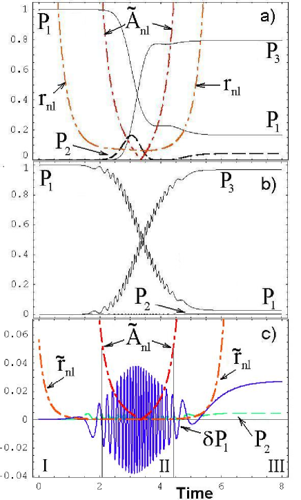
Figure 2: (Color online)Population dynamics and the adiabatic parameters $A_{nl}$, $r_{nl}$. Tildes over the parameters denote division by 10 (in order to fit into the scale): $\tilde{X}\equiv X/10$. $P_{1,2,3}$: populations of $|a\rangle$, $|e\rangle$, $|g\rangle$, i.e. $x_{1}^{2}+y_{1}^{2},2(x_{2}^{2}+y_{2}^{2}),2(x_{3}^{2}+y_{3}^{2})$ correspondingly. Solid lines: $P_{1,3}$; dashed lines: $P_{2}$ (should be zero in the dark state); dot-dashed lines: the adiabatic parameters. (a) The same numerical example as in Ref.Pu ; $t_{p}=3.8,t_{d}=3$, $\Omega_{0}=5$. Note the dynamics of $P_{2}$: at $t\approx 3$ it deviates from zero considerably. Parameter $r_{nl}$ suggests adiabatic evolution at $1.5<t<4.5$. Parameter $A_{nl}$ is huge (almost two orders of magnitude larger than $r_{nl}$), suggesting nonadiabatic evolution. Note that $H,I_{1,3}$ remains zero. (b,c) $\Omega_{0}=100$, other parameters are the same as in the previous numerical example; (b) Population dynamics. High-frequency oscillations are seen in $P_{1,2,3}$ (c) Dynamics of adiabatic parameters $A_{nl},r_{nl}$ and deviation of $P_{1}$ from its value in the dark state ($P_{1}^{0}$): $\delta P_{1}=P_{1}-P_{1}^{0}$. Three stages of nonlinear STIRAP can be defined (I-III), with only the second stage being adiabatic. In the first stage ($t\lesssim 2.5$) $A_{nl}$ is large, so system acquires some action. At the second stage ($2.5\lesssim t\lesssim 4.5$) $A_{nl}$ is small, and population transfer proceeds (with approximate conservation of the acquired action). At the third stage (from $t\approx 4.5$), adiabaticity is broken again. Predictions of $A_{nl}$ are better than that of $r_{nl}$.

Fig. 1c presents phase portraits of this Hamiltonian. There is a stable fixed point which corresponds to the dark state: $z=\frac{1}{2}\ln\large[\frac{2\Omega_{d}}{\Omega_{d}+\Omega_{e}}\large],\quad\phi=\pi$. As time increases, it goes from $z=0$ to $-\infty$. For small-amplitude oscillations, linearization around the stable fixed point gives the frequency $\omega=\frac{1}{2}(\Omega_{d}\Omega_{e})^{1/2}.$ Adiabatic evolution requires change of this frequency $\delta\omega$ at one period of unperturbed motion to be much less than frequency itself AKN ; how : $|\delta\omega|\ll|\omega|$. Since $\delta\omega\approx\dot{\omega}*2\pi/\omega$, we have the following criteria: $|\dot{\omega}|\ll\omega^{2}/2\pi$, or $|\Omega_{e}\dot{\Omega}_{d}+\dot{\Omega}_{e}\Omega_{d}|\ll\frac{1}{2\pi}(\Omega_{d}\Omega_{e})^{3/2},$ or

$$A_{nl}\equiv 2\pi|\Omega_{e}\dot{\Omega}_{d}+\dot{\Omega}_{e}\Omega_{d}|/(\Omega_{d}\Omega_{e})^{3/2}\ll 1$$ (4)

It can be seen from Fig. 2 that $A_{nl}$ works sufficiently better than $r_{nl}$ of Pu ($A_{nl}$ is typically an order of magnitude larger than $r_{nl}$ in this numerical example). For one-and-half d.o.f. Hamiltonian systems, the criterion $|\delta\omega|\ll|\omega|$ as described above is reliable to analyze adiabaticity.

In systems with several degrees of freedom, situation is much more complicated. Even stability at fixed parameters is highly nontrivial issue. Indeed, let us now consider the case $\Delta\neq 0$ (or $\Delta=0$, but $H\neq 0$), where we cannot utilize the trick with the energy manifold, so the system with fixed parameters $\Omega_{p,d}$ has 2 d.o.f. We make several canonical transformations to reduce the Hamiltonian system to a 2 d.o.f. one, and shift the origin to the point corresponding to the dark state (see AV ). We get the Hamiltonian in new variables $q_{1,2},p_{1,2}$

$${\cal H}=\Omega_{p}[q_{1}^{2}+p_{1}^{2}+q_{2}^{2}+p_{2}^{2}]p_{1}-\frac{\Omega_{d}}{2}q_{1}q_{2}-\frac{\Omega_{e}}{2}p_{1}p_{2}-\frac{\Delta}{2}(q_{1}^{2}+p_{1}^{2}).$$ (5)

One may transform the quadratic part of the Hamiltonian to its normal form: sum of two linear oscillators, and neglect the cubic part, obtaining therefore two uncoupled oscillators (with frequencies $\omega_{\pm}$). However, such straightforward approach is dangerous at low-order resonances between $\omega_{\pm}$. The 1:1 resonance happens at $\Delta=0$, while 1:2 resonance at $\Delta=\sqrt{\Omega_{d}\Omega_{e}/8}$. Consider firstly 1:1 resonance ($\Delta=0$). We introduce a parameter $\theta$ as $\Omega_{d}=\Omega_{e}\cos\theta,\quad\Omega_{p}=\Omega_{e}\sin\theta/2\sqrt{2},\quad 1>\cos\theta>0,$ and divide the Hamiltonian (5) by $\Omega_{e}$: ${\cal H}=\frac{\sin\theta}{2\sqrt{2}}(q_{1}^{2}+p_{1}^{2}+q_{2}^{2}+p_{2}^{2})p_{1}-\frac{\cos\theta}{2}q_{1}q_{2}-\frac{1}{2}p_{1}p_{2}.$

We transform the quadratic part of the Hamiltonian to the normal form by means of linear transformations and obtain (retaining old notations for new variables)

$$H=H_{2}+H_{3}=\frac{1}{2}\sqrt{\cos\theta}(p_{2}q_{1}-p_{1}q_{2})+H_{3},$$ (6)

where $H_{3}$ consists of cubic terms (for 1:1 resonance, it is convenient to use series in $p_{2}q_{1}-p_{1}q_{2}$, $p_{1}^{2}+p_{2}^{2}$, $q_{1}^{2}+q_{2}^{2}$. Hamiltonians which depends only on such combinations of variables are also called normal forms). We need to get rid of the cubic terms in the Hamiltonian. To this end, we fulfill a nonlinear canonical transformation using a generating function $K_{3}$ which is a homogenous polynomial of the third order in old coordinates and new momenta: $K_{3}=\alpha q_{1}^{2}q_{2}+\beta P_{2}^{2}q_{2}+zP_{1}^{2}q_{2}+\gamma q_{2}^{3}+fP_{1}P_{2}q_{1}.$ For the coefficients $\alpha,\beta,\gamma,f,z$ in $K_{3}$, we get a system of linear equations; the transformation defined by $K_{3}$ kills all cubic terms, while quadratic part remains the same; at the same time, quartic terms emerge: we get the Hamiltonian $H=\frac{1}{2}\sqrt{\cos\theta}(P_{2}Q_{1}-P_{1}Q_{2})+H_{4}+..,$ where $H_{4}$ contains the quartic terms. Generally, it is not possible to kill all quartic terms AKN . We need to transform $H_{4}$ to the normal form. However, we can proceed in a simpler (but equivalent) way.

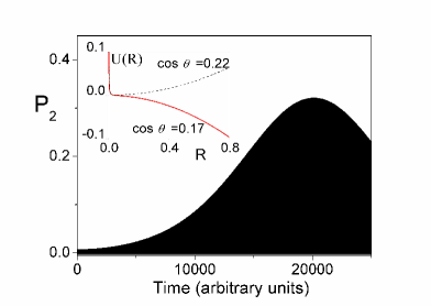
Figure 3: (Color online) Instability in 1:1 resonance. Dynamics of population of the excited state $P_{2}$ (which should be zero in the dark state) is shown. Parameters: $\Omega_{p}=2.0$, $\Omega_{d}=1.0$ ($\cos\theta\approx 0.17<0.2$, $\Omega_{p}>\sqrt{3}\Omega_{d}$). Instability develops on long timescales: we start with small deviation from the dark state, but the deviation grows and reach very large values. With $\cos\theta>0.2$ (not shown), initial deviation do not grow much: it slowly oscillates about the equilibrium of the effective potential of (7). The curve $P_{2}(t)$ is filled by oscillations with frequency $\frac{1}{2}\sqrt{\Omega_{d}\Omega_{e}}$ which are not seen in this scale. Inset shows two effective potentials of (7) at $J=0.001$ and two different values of $\theta$; solid line with $\cos\theta=0.17<0.2$ corresponds to the unbounded motion (instability).

We change to polar coordinates in $Q_{1},Q_{2}$ plane making a transformation $Q_{1}=R\cos\xi,\quad Q_{2}=R\sin\xi,\quad P_{1}=P\cos\xi-\frac{J\sin\xi}{R},\quad P_{2}=P\sin\xi+\frac{J\cos\xi}{R},$ and then average over the (fast) angle $\xi$. We obtain the following effective Hamiltonian:

$$F=\frac{1}{2}J-\frac{J\kappa_{\theta}^{2}}{8}\left[\frac{A_{P}}{2}\large(P^{2}+\frac{J^{2}}{R^{2}}\large)+R^{2}A_{R}\right],$$ (7)

where $A_{P}=\frac{10\cos^{2}\theta+10\cos\theta+4}{3},\quad A_{R}=5\cos\theta-1$, $\kappa_{\theta}=\frac{\sin\theta}{\sqrt{2}\sqrt{\cos\theta}}$. In this Hamiltonian, $J$ is constant. Therefore, it is an integrable system for a pair of canonically conjugated variables $P,R$. It is not difficult to understand its dynamics: (7) is merely a Hamiltonian of a particle in the potential $U(R)=\frac{J^{2}A_{P}}{2R^{2}}+A_{R}R^{2}$ (indeed, only the expression in the square brackets in (7) is important for dynamics). The effective potentials $U(R)$ are shown in the inset of Fig.(3). For $\cos\theta>\frac{1}{5}$, the system (7) has a single fixed point, while for $\cos\theta<\frac{1}{5}$ there are no fixed points. In the latter case (corresponding to $\Omega_{p}/\Omega_{d}>\sqrt{3}$), a phase point initially placed close to $R=0$ will slowly move from the origin to large values of $R$. The dark state corresponds to $R=0$, therefore this case implies dynamical instability due to 1:1 resonance. The instability is slow (see Fig.3), nevertheless it is physically important: it develops on the same timescales as that used in Javanainen . We checked that crossing the critical $\cos\theta=\frac{1}{5}$ value results in onset of dynamical instability, in accordance with the effective potential (7). Physically, $\cos\theta<\frac{1}{5}$ means that most of the population is in $|g\rangle$ state. In this region, the dark state is unstable: deviations from it slowly grows with time, populating $|e\rangle$ state considerably, which would lead to spontaneous emission in real experiments. To be more precise, deviations from the dark state firstly oscillate in time with frequency $\frac{1}{2}\sqrt{\Omega_{d}\Omega_{e}}$ and small amplitude, and then the amplitude of oscillations slowly grows. Thus, one may see periodic bursts of spontaneous emission each time the deviations reach their maxima (i.e., with a time period $T\sim 1/\sqrt{\Omega_{d}\Omega_{e}}$).

Let us now turn to 1:2 resonance. Usually, its analysis is much simpler than that of 1:1 and 1:3 resonances, as it involves only cubic terms. Unfortunately, in our case this resonance is also degenerate. In 1:2 resonance, we can bring the Hamiltonian to the resonance normal form

$$H_{res}=\omega_{1}R_{1}+\omega_{2}R_{2}+\kappa R_{1}^{1/2}R_{2}\sin(\phi_{1}+2\phi_{2}),$$ (8)

where $(R_{i},\phi_{i})$ are symplectic polar coordinates (action-angle variables of $H_{2}$: $P_{i}=\sqrt{2R_{i}}\sin\phi_{i},\quad Q_{i}=\sqrt{2R_{i}}\cos\phi_{i}$), $\kappa$ is some coefficient, the frequencies $\omega_{1}$ and $\omega_{2}$ are in 1:2 resonance: $\omega_{1}+2\omega_{2}=0$ (so, $\omega_{1}\omega_{2}<0$). The resonance normal form is obtained by averaging out all terms in $H_{3}$ except the resonance one (which depends on the resonance phase $\gamma\equiv\phi_{1}+2\phi_{2}$) AKN . The resonance normal form is integrable. Provided certain conditions of generality are fulfilled, the equilibrium of the original system (i.e., the dark state) is stable or unstable simultaneously with the equilibrium of the resonance normal form (i.e., $R_{1,2}=0$). For 1:2 resonance, a condition of generality is $\kappa\neq 0$; with $\omega_{1}\omega_{2}<0$ and $\kappa\neq 0$, the equilibrium is unstable AKN . In our case, $\kappa=0$, therefore this source of instability is absent in the system. Still, the degeneracy $\kappa=0$ does not guarantee stability, but designates that possible instabilities, if exist, are very slow.

It is important to emphasize that stability and adiabaticity are two different issues. Adiabatic invariance in systems with several degrees of freedom is also remarkably nontrivial Rbil . Main difficulties come from passage through resonances; in case our system stays away from low-order resonances as parameters are changed, we can consider it as two decoupled oscillators and generalize the adiabatic condition (4) straightforwardly, see AV .

Here, we analyzed low-order resonances of the nonlinear $\Lambda$ system; found nonlinear instabilities of the dark state; found cases of complete integrability and improved adiabatic conditions for nonlinear STIRAP. The suggested method is generalized to systems with mean-field collisional interactions in AV . Briefly, theory of nonlinear STIRAP is developed.

A.P.I. was supported by JSPS and 21st Century COE program on “Coherent Optical Science”. This work was also supported by Grants-in-Aid No. 16-04315 from MEXT, Japan. A.P.I. acknowledges help of A.A.Vasiliev, discussions with A.I. Neishtadt, and thanks J.Bohn for his kind invitation to visit JILA, where this manuscript was finished.

References

- (1) P. Ehrenfest, Phil. Magazine 33, 500 (1917); D. Bohm, Quantum Theory (Prentice Hall, NJ, 1951); K.P. Marzlin and B.C. Sanders, Phys. Rev. Lett. 93, 160408 (2004).
- (2) L. P. Pitaevskii and S. Stringari, Bose-Einstein condensation (Clarendon Press, Oxford, 2003).
- (3) O.Zobay, B.M. Garraway, Phys. Rev. A 61, 033603 (2000); B. Wu and Q. Niu, Phys. Rev. A 61, 023402 (2000); J. Liu et al, Phys. Rev. A 66, 023404 (2002); D. Diakonov, L. M. Jensen, C.J. Pethick, and H. Smith, Phys.Rev. A 66, 013604 (2002); H.Saito and M.Ueda, Phys. Rev. Lett. 93, 220402 (2004); V. V. Konotop, P. G. Kevrekidis, M. Salerno, Phys. Rev. A 72, 023611 (2005); D. Witthaut, E. M. Graefe, and H. J. Korsch, Phys. Rev. A 73, 063609 (2006); V. A. Brazhnyi, V. V. Konotop, V. Kuzmiak, and V. S. Shchesnovich, Phys. Rev. A 76, 023608 (2007).
- (4) A.P.Itin et al, Physica D 232, 108 (2007); A.P.Itin, S.Watanabe, Phys. Rev. E 76, 026218 (2007); see also http://power1.pc.uec.ac.jp/alx_it
- (5) S.B. McKagan et al, Phys. Rev. A 74, 013612 (2006).
- (6) H.Pu et al, Phys.Rev.Lett. 98, 050406 (2007).
- (7) M. Mackie et al, Phys. Rev. Lett 84, 3803 (2000).
- (8) F. T. Hioe, Phys. Lett. A 99, 150 (1983); N. V. Vitanov et al, Adv. At. Mol. Opt. Phys., 46, 55 (2001).
- (9) K.Winkler et al, Phys.Rev.Lett 95, 063202 (2005); D. J. Heinzen et al, Phys. Rev. Lett. 84, 5029 (2000).
- (10) A.Ishkhanyan et al, in Interactions in Ultracold Gases, ed. by M.Weidemuller, K.Zimmermann (Wiley-Vch, Berlin, 2003);
- (11) V.I.Arnold, V.V.Kozlov, and A.I.Neishtadt, Mathematical aspects of classical and celestial mechanics (Third Edition, Springer, Berlin, 2006), and references therein.
- (12) J.J. Duistermaat, in Bifurcation Theory and Applications, ed. by L. Salvadori, Lect. Notes Math. 1057, 57 (Springer-Verlag, Berlin, 1984).
- (13) We estimate influence of movement of the fixed point to be of the same order as change in the frequency; the adiabatic condition is therefore the same as in the case of a stationary fixed point; generally, it is not always so.
- (14) A.P.Itin et al, in preparation.
- (15) A.I.Neishtadt, Prikl.Mat.Mekh. 39, 1331 (1975); A.P.Itin, A.I. Neishtadt, A.A. Vasiliev, Physica D 141, 281 (2000); A.P.Itin, A.A. Vasiliev, A.I.Neishtadt, Phys. Lett. A 291, 133 (2001); A.P.Itin, Plasma Physics Reports 28, 592 (2002); A.P.Itin, Phys. Rev. E 67, 026601 (2003).