Effective Lagrangian approach to fermion electric dipole moments induced by a CP–violating $WW\gamma$ vertex

Abstract

The one–loop contribution of the two CP–violating components of the $WW\gamma$ vertex, $\tilde{\kappa}_{\gamma}W^{+}_{\mu}W^{-}_{\nu}\tilde{F}^{\mu\nu}$ and $(\tilde{\lambda}_{\gamma}/m^{2}_{W})W^{+}_{\mu\nu}W^{-\nu}_{\ \ \rho}\tilde{F}^{\rho\mu}$, on the electric dipole moment (EDM) of fermions is calculated using dimensional regularization and its impact at low energies reexamined in the light of the decoupling theorem. The Ward identities satisfied by these couplings are derived by adopting a $SU_{L}(2)\times U_{Y}(1)$–invariant approach and their implications in radiative corrections discussed. Previous results on $\tilde{\kappa}_{\gamma}$, whose bound is updated to $|\tilde{\kappa}_{\gamma}|<5.2\times 10^{-5}$, are reproduced, but disagreement with those existing for $\tilde{\lambda}_{\gamma}$ is found. In particular, the upper bound $|\tilde{\lambda}_{\gamma}|<1.9\times 10^{-2}$ is found from the limit on the neutron EDM, which is more than 2 orders of magnitude less stringent than that of previous results. It is argued that this difference between the $\tilde{\kappa}_{\gamma}$ and $\tilde{\lambda}_{\gamma}$ bounds is the one that might be expected in accordance with the decoupling theorem. This argument is reinforced by analyzing careful the low–energy behavior of the loop functions. The upper bounds on the $W$ EDM, $|d_{W}|<6.2\times 10^{-21}\ e\cdot cm$, and the magnetic quadrupole moment, $|\tilde{Q}_{W}|<3\times 10^{-36}\ e\cdot cm^{2}$, are derived. The EDM of the second and third families of quarks and charged leptons are estimated. In particular, EDM as large as $10^{-20}\ e\cdot cm$ and $10^{-21}\ e\cdot cm$ are found for the $t$ and $b$ quarks, respectively.

I Introduction

Very important information about the origin of CP violation may be extracted from EDMs of elementary particles. This elusive electromagnetic property is very interesting, as it represents a net quantum effect in any renormalizable theory. In the standard model (SM), the only source of CP violation is the Cabbibo–Kobayashi–Maskawa (CKM) phase, which however has a rather marginal impact on flavor–diagonal processes such as the EDM of elementary particles DS . In fact, the EDM of both fermions and the $W$ gauge boson first arises at the three–loop level EDMQW1 ; EDMQW2 . As far as the magnetic quadrupole moment of the $W$ boson is concerned, it receives a tiny contribution at the two–loop level in the SMMQMW . Although they are extremely suppressed in the SM, the EDMs can be very sensitive to new sources of CP violation, as it was shown recently for the case of the $W$ boson in a model–independent manner using the effective Lagrangian techniqueTT1 ; HHPTT . Indeed, EDMs can receive large contributions from many SM extensionsBM , so the scrutiny of these properties may provide relevant information to our knowledge of CP violation, which still remains a mystery.

In this paper, we are interested in studying the impact of a CP–violating $WW\gamma$ vertex on the EDM of charged leptons and quarks. As it was shown by Marciano and QueijeiroMQ , the CP–odd electromagnetic properties of the $W$ boson can induce large contributions on the EDM of fermions. Beyond the SM, the CP–violating $WW\gamma$ vertex can be induced at the one–loop level by theories that involve both left– and right–handed currents with complex phasesTT2 ; HHPTT , as it occurs in left–right symmetric modelsLRSM . Two–loop effects can arise from Higgs boson couplings to $W$ pairs with undefined CP structure TT1 . However, in this work, instead of focusing on a specific model, we will parametrize this class of effects in a model–independent manner via the effective Lagrangian approachEL , which is suited to describe those new physics effects that are quite suppressed or forbidden in the SM. The phenomenological implications of both the CP–even and the CP–odd trilinear $WWV$ ($V=\gamma,Z$) couplings have been the subject of intense study in diverse contexts using the effective Lagrangian approach Ha ; Wudka . The static electromagnetic properties of the $W$ gauge boson can be parametrized by the following effective Lagrangian:

$${\cal L}_{WW\gamma}=-ie\Big{(}\Delta\kappa_{\gamma}F_{\mu\nu}W^{-\mu}W^{+\nu}+\frac{\lambda_{\gamma}}{m^{2}_{W}}W^{+}_{\mu\nu}W^{-\nu}_{\ \ \rho}F^{\rho\mu}+\tilde{\kappa}_{\gamma}W^{+}_{\mu}W^{-}_{\nu}\tilde{F}^{\mu\nu}+\frac{\tilde{\lambda}_{\gamma}}{m^{2}_{W}}W^{+}_{\mu\nu}W^{-\nu}_{\ \ \rho}\tilde{F}^{\rho\mu}\Big{)},$$ (1)

where $W^{\pm}_{\mu\nu}=\partial_{\mu}W^{\pm}_{\nu}-\partial_{\nu}W^{\pm}_{\mu}$ and $\tilde{F}_{\mu\nu}=(1/2)\epsilon_{\mu\nu\alpha\beta}F^{\alpha\beta}$. The sets of parameters $(\Delta\kappa_{\gamma},\lambda_{\gamma})$ and $(\tilde{\kappa}_{\gamma},\tilde{\lambda}_{\gamma})$ define the CP–even and CP–odd static electromagnetic properties of the $W$ boson, respectively. The magnetic dipole moment ($\mu_{W}$) and the electric quadrupole momente ($Q_{W}$) are defined by Ha

$$\mu_{W}=\frac{e}{2m_{W}}(2+\Delta\kappa_{\gamma}+\lambda_{\gamma}),\ \ \ Q_{W}=-\frac{e}{m^{2}_{W}}(1+\Delta\kappa_{\gamma}-\lambda_{\gamma}).$$ (2)

On the other hand, the electric dipole moment ($d_{W}$) and the magnetic quadrupole moment ($\tilde{Q}_{W}$) are defined by Ha

$$d_{W}=\frac{e}{2m_{W}}(\tilde{\kappa}_{\gamma}+\tilde{\lambda}_{\gamma}),\ \ \ \ \tilde{Q}_{W}=-\frac{e}{m^{2}_{W}}(\tilde{\kappa}_{\gamma}-\tilde{\lambda}_{\gamma}).$$ (3)

The dimension–four interactions of the above Lagrangian are induced after spontaneous symmetry breaking by the following dimension–six $SU_{L}(2)\times U_{Y}(1)$–invariant operators:

$${\cal O}_{WB}=\frac{\alpha_{WB}}{\Lambda^{2}}\Big{(}\Phi^{\dagger}\frac{\sigma^{a}}{2}\Phi\Big{)}W^{a\mu\nu}B_{\mu\nu}$$ (4)

$$\tilde{{\cal O}}_{WB}=\frac{\tilde{\alpha}_{WB}}{\Lambda^{2}}\Big{(}\Phi^{\dagger}\frac{\sigma^{a}}{2}\Phi\Big{)}W^{a\mu\nu}\tilde{B}_{\mu\nu},$$ (5)

whereas those interactions of dimension six are generated by the following $SU_{L}(2)$–invariants:

$${\cal O}_{W}=\frac{\alpha_{W}}{\Lambda^{2}}\Big{(}\frac{\epsilon_{abc}}{3!}W^{a\mu}_{\ \ \nu}W^{b\nu}_{\ \ \rho}W^{c\rho}_{\ \ \mu}\Big{)},$$ (6)

$$\tilde{{\cal O}}_{W}=\frac{\tilde{\alpha}_{W}}{\Lambda^{2}}\Big{(}\frac{\epsilon_{abc}}{3!}W^{a\mu}_{\ \ \nu}W^{b\nu}_{\ \ \rho}\tilde{W}^{c\rho}_{\ \ \mu}\Big{)},$$ (7)

where $W^{a}_{\mu\nu}$ and $B_{\mu\nu}$ are the tensor gauge fields associated with the $SU_{L}(2)$ and $U_{Y}(1)$ groups, respectively. In addition, $\Phi$ is the Higgs doublet, $\Lambda$ is the new physics scale, and the $\tilde{\alpha}_{i}$ are unknown coefficients, which can be determined if the underlying theory is known. As we will see below, the presence of the Higgs doublet in the ${\cal O}_{WB}$ and $\tilde{{\cal O}}_{WB}$ operators, as well as its absence in ${\cal O}_{W}$ and $\tilde{{\cal O}}_{W}$, has important physical implications at low energies. In the following, we will focus on the CP–violating interactions. Introducing the dimensionless coefficients $\tilde{\epsilon}_{i}=(v/\Lambda)^{2}\tilde{\alpha}_{i}$, with $v$ the Fermi scale, it is easy to show that $\tilde{\kappa}_{\gamma}=-(c_{W}/2s_{W})\tilde{\epsilon}_{WB}$ and $\tilde{\lambda}_{\gamma}=-(e/4s_{W})\tilde{\epsilon}_{W}$, with $s_{W}(c_{W})$ the sine(cosine) of the weak angle. The impact of the $\tilde{{\cal O}}_{WB}$ operator on the EDM of fermions, $d_{f}$, was studied in Ref.MQ . The experimental limits on the EDM of the electron and neutron were used by the authors to impose a bound on the $\tilde{\kappa}_{\gamma}$ parameter . It was found that the best bound arises from the limit on the neutron EDM $d_{n}$. In this paper, besides reproducing this calculation using dimensional regularization and updating the bound on $\tilde{\kappa}_{\gamma}$ and $d_{W}$, we will derive an upper bound on the magnetic quadrupole moment $\tilde{Q}_{W}$, which, to our knowledge, has not been presented in the literature.

On the other hand, the contribution of the $\tilde{{\cal O}}_{W}$ operator to the EDM of fermions has also been studied previously by several authors DRS ; MANYRS . Although this operator gives a finite contribution to $d_{f}$, it has been argued by the authors of Ref.MANYRS that such a contribution is indeed ambiguous, as it is regularization–scheme dependent. The authors of Ref.MANYRS carried out a comprehensive analysis by calculating the $\tilde{{\cal O}}_{W}$ contribution to $d_{f}$ using several regularization schemes, such as dimensional, form–factor, Paulli–Villars–regularization, and the Cutoff method. They show that the result differs from one scheme to other. In this paper, we reexamine this contribution using the dimensional regularization scheme. We argue that the result thus obtained is physically acceptable because it satisfies some low energy requirements that are inherent to the Appelquist–Carazzone decoupling theorem DT . In particular, we will emphasize the relative importance of the $\tilde{{\cal O}}_{WB}$ and $\tilde{{\cal O}}_{W}$ operators when inserted into a loop to estimate their impact on a low–energy observable as the EDM of the electron or the neutron. As we will see below, the $\tilde{{\cal O}}_{WB}$ operator induces nondecoupling effects, whereas $\tilde{{\cal O}}_{W}$ is of decoupling nature. As a consequence, the constraints obtained from the neutron EDM are more stringent for $\tilde{{\cal O}}_{WB}$ than for $\tilde{{\cal O}}_{W}$, in contradiction with the results of Ref.MANYRS where bounds of the same order of magnitude are found. Below we will argue on the consistence of our results by analyzing more closely some peculiarities of these operators in the light of the decoupling theorem. Although the $\tilde{{\cal O}}_{W}$ contribution is insignificant compared with the one of $\tilde{{\cal O}}_{WB}$ for light fermions, it is very important to stress that both operators can be equally important at high energies. Indeed, we will see that for the one–loop $\bar{t}t\gamma$ and $\bar{b}b\gamma$ vertices, the $\tilde{{\cal O}}_{W}$ contribution is as large as or larger than the effect of $\tilde{{\cal O}}_{WB}$. We will see below that as a consequence of the decoupling nature of $\tilde{{\cal O}}_{W}$, the bound obtained on $\tilde{\lambda}_{\gamma}$ from the neutron EDM is two orders of magnitude less stringent than that on $\tilde{\kappa}_{\gamma}$.

Another important goal of this work is to use our bounds on the $\tilde{\kappa}_{\gamma}$ and $\tilde{\lambda}_{\gamma}$ parameters to predict, besides the CP–odd electromagnetic properties of the $W$ gauge boson, the EDM of the second and third families of charged leptons and quarks. We believe that the heaviest particles, as the $W$, $\tau$, $b$, and $t$, could eventually be more sensitive to new physics effects associated with CP violation. In addition, we will exploit the $SU_{L}(2)\times U_{Y}(1)$ invariance of our framework to derive limits on the $\tilde{\kappa}_{Z}$ and $\tilde{\lambda}_{Z}$ parameters associated with the CP–odd $WWZ$ vertex.

The paper has been organized as follows. In Sec. II, the Feynman rule for the CP–odd $WW\gamma$ vertex is presented. We will focus on the gauge structure of the part coming from the $\tilde{{\cal O}}_{W}$ operator. In particular, we will show how this operator leads to a gauge–independent result even in the most general case when all particles in the $WW\gamma$ vertex are off–shell. Sec. III is devoted to derive the amplitudes for the on–shell one–loop $\bar{l}l\gamma$ and $\bar{q}q\gamma$ vertices, induced by the CP–odd $WW\gamma$ coupling. In Sec. IV, the bounds on the $\tilde{\kappa}_{\gamma}$ and $\tilde{\lambda}_{\gamma}$ parameters are derived and used to predict the EDM of the SM particles. Finally, in Sec. V the conclusions are presented.

II The anomalous CP–violating $WW\gamma$ vertex

In this section, we present the Feynman rule for the $WW\gamma$ vertex induced by the effective operators given in Eqs. (5) and (7). The $\tilde{{\cal O}}_{WB}$ term can be written in the unitary gauge as follows:

$$\tilde{{\cal O}}_{WB} = -\frac{1}{4}\tilde{\epsilon}_{WB}\tilde{B}_{\mu\nu}W^{3\mu\nu}+\cdots,$$ (8)

$$= -ie\Big{(}\frac{c_{W}}{2s_{W}}\tilde{\epsilon}_{WB}\Big{)}\tilde{F}_{\mu\nu}W^{-\mu}W^{+\nu}+\cdots,$$

where

$$\tilde{B}_{\mu\nu} = c_{W}\tilde{F}_{\mu\nu}-s_{W}\tilde{Z}_{\mu\nu},$$ (9)

$$W^{3}_{\mu\nu} = s_{W}F_{\mu\nu}+c_{W}Z_{\mu\nu}+ig(W^{-}_{\mu}W^{+}_{\nu}-W^{+}_{\mu}W^{-}_{\nu}).$$ (10)

On the other hand, the $\tilde{{\cal O}}_{W}$ term is given by

$$\tilde{{\cal O}}_{W} = \frac{i\tilde{\alpha}_{W}}{\Lambda^{2}}\hat{W}^{+\nu\lambda}\hat{W}^{-\mu}_{\nu}\tilde{W}^{3}_{\lambda\mu},$$ (11)

$$= ie\Big{(}\frac{e}{4s_{W}}\tilde{\epsilon}_{W}\Big{)}\Big{(}\frac{1}{m^{2}_{W}}\Big{)}W^{+\nu\lambda}W^{-\mu}_{\nu}\tilde{F}_{\lambda\mu}+\cdots,$$

where

$$\hat{W}^{+}_{\mu\nu}=D_{\mu}W^{+}_{\nu}-D_{\nu}W^{+}_{\mu}+igc_{W}(W^{+}_{\mu}Z_{\nu}-W^{+}_{\nu}Z_{\mu}),$$ (12)

with $D_{\mu}=\partial_{\mu}-ieA_{\mu}$ the electromagnetic covariant derivative and $\hat{W}^{-}_{\mu\nu}=(\hat{W}^{+}_{\mu\nu})^{\dagger}$.

Using the notation shown in Fig.1, the vertex function associated with the $WW\gamma$ coupling can be written as

$$\tilde{\Gamma}^{WW\gamma}_{\lambda\rho\mu}(k_{1},k_{2},k_{3})=ie\tilde{\kappa}_{\gamma}\Gamma^{\tilde{\cal O}_{WB}}_{\lambda\rho\mu}(k_{1})+\frac{ie\tilde{\lambda}_{\gamma}}{m^{2}_{W}}\Gamma^{\tilde{\cal O}_{W}}_{\lambda\rho\mu}(k_{1},k_{2},k_{3}),$$ (13)

where

$$\Gamma^{\tilde{\cal O}_{WB}}_{\lambda\rho\mu}(k_{1})=\epsilon_{\mu\lambda\rho\eta}k^{\eta}_{1},$$ (14)

$$\Gamma^{\tilde{\cal O}_{W}}_{\lambda\rho\mu}(k_{1},k_{2},k_{3})=(-k_{2}\cdot k_{3}\epsilon_{\lambda\rho\mu\eta}+k_{2\rho}\epsilon_{\lambda\mu\eta\sigma}k^{\sigma}_{3}-k_{3\lambda}\epsilon_{\rho\mu\eta\sigma}k^{\sigma}_{2})k^{\eta}_{1}.$$ (15)

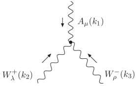
Figure 1: The trilinear CP–odd $WW\gamma$ vertex.

We now proceed to derive the Ward identities that are satisfied by these vertex functions. In particular, we will show that as a consequence of these identities, the $\Gamma^{\tilde{\cal O}_{W}}_{\lambda\rho\mu}(k_{1},k_{2},k_{3})$ vertex cannot introduce a gauge–dependent contribution in any loop amplitude. From Eq.(15) it is easy to show that this vertex satisfies the following simple Ward identities:

$$k^{\mu}_{1}\Gamma^{\tilde{\cal O}_{W}}_{\lambda\rho\mu}(k_{1},k_{2},k_{3}) = 0,$$ (16)

$$k^{\lambda}_{2}\Gamma^{\tilde{\cal O}_{W}}_{\lambda\rho\mu}(k_{1},k_{2},k_{3}) = 0,$$ (17)

$$k^{\rho}_{3}\Gamma^{\tilde{\cal O}_{W}}_{\lambda\rho\mu}(k_{1},k_{2},k_{3}) = 0,$$ (18)

which arise as a direct consequence of the invariance of $\tilde{{\cal O}}_{W}$ under the $SU_{L}(2)$ group. Since all the $SU_{L}(2)\times U_{Y}(1)$ invariants of dimension higher than four cannot be affected by the gauge–fixing procedure applied to the dimension–four theory, any possible gauge dependence necessarily must arise from the longitudinal components of the gauge field propagators through the $\xi$ gauge parameter. Gauge–independence means independence with respect to this parameter. It is clear now that as a consequence of the above Ward identities, the $\Gamma^{\tilde{\cal O}_{W}}_{\lambda\rho\mu}(k_{1},k_{2},k_{3})$ contribution to a multi–loop amplitude is gauge–independent, as there are no contributions from the longitudinal components of the propagators and thus it cannot depend on the $\xi$ gauge parameter. Of course, the complete amplitude maybe gauge–dependent due to the presence of other gauge couplings. However, when this anomalous vertex is the only gauge coupling involved in a given amplitude, as it is the case of the one–loop electromagnetic properties of a fermion $f$, the corresponding form factors are manifestly gauge independent. This means that for all practical purpose, the contribution of this operator to a given amplitude can be calculated using the Feynman–’tHooft gauge ($\xi=1$). We will see below that, as a consequence of these Ward identities, the contribution of this operator to the fermion EDM is not only manifestly gauge–independent, but also free of ultraviolet divergences. The same considerations apply to the CP–even counterpart ${\cal O}_{W}$. These results are also valid for the $WWZ$ coupling. As far as the $\Gamma^{\tilde{\cal O}_{WB}}_{\lambda\rho\mu}(k_{1})$ vertex is concerned, it also is subject to satisfy certain Ward identities that arise as a consequence of the $SU_{L}(2)\times U_{Y}(1)$–invariance of the $\tilde{{\cal O}}_{WB}$ operator. However, these constraints, in contrast with the ones satisfied by the $\Gamma^{\tilde{\cal O}_{W}}_{\lambda\rho\mu}(k_{1})$ vertex, are not simple due to the presence of pseudo Goldstone bosons. These Ward identities are relations between the $WW\gamma$ and the $G^{\pm}W^{\mp}\gamma$ vertices, which are given by

$$k^{\mu}_{1}\Gamma^{\tilde{\cal O}_{WB}}_{\lambda\rho\mu}(k_{1}) = 0,$$ (19)

$$k^{\lambda}_{2}\Gamma^{\tilde{\cal O}_{WB}}_{\lambda\rho\mu}(k_{1}) = m_{W}\Gamma^{G^{+}W^{-}\gamma}_{\mu\rho}(k_{1},k_{3}),$$ (20)

$$k^{\rho}_{3}\Gamma^{\tilde{\cal O}_{WB}}_{\lambda\rho\mu}(k_{1}) = m_{W}\Gamma^{G^{-}W^{+}\gamma}_{\mu\lambda}(k_{1},k_{2}),$$ (21)

where

$$\Gamma^{G^{+}W^{-}\gamma}_{\mu\rho}(k_{1},k_{3}) = -\frac{1}{m_{W}}\epsilon_{\mu\rho\alpha\beta}k^{\alpha}_{3}k^{\beta}_{1},$$ (22)

$$\Gamma^{G^{-}W^{+}\gamma}_{\mu\lambda}(k_{1},k_{2}) = -\frac{1}{m_{W}}\epsilon_{\mu\rho\alpha\beta}k^{\alpha}_{2}k^{\beta}_{1}.$$ (23)

These results are also valid for the $WWZ$ vertex. They also apply to the CP–even counterpart ${\cal O}_{WB}$.

III The one–loop induced CP–violating $\bar{f}f\gamma$ vertex

We now turn to calculating the contribution of the $\tilde{{\cal O}}_{WB}$ and $\tilde{{\cal O}}_{W}$ operators to the EDM of a $f$ fermion. The EDM of $f$ is induced at the one–loop level through the diagram shown in Fig.2. It is convenient to analyze separately the contribution of each operator, as they possess different features that deserve to be contrasted. To calculate the loop amplitudes we have chosen the dimensional regularization scheme, as it is a gauge covariant method which has probed to be appropriate in theories that are nonrenormalizable in the Dyson’s sense W . This framework has been used successfully in many loop calculations within the context of effective field theories MANY . Although the Feynman parametrization technique is the adequate method to calculating on–shell electromagnetic form factors, we will use also the Passarino–Veltman PV covariant decomposition in the case of the $\tilde{{\cal O}}_{W}$ contribution, in order to clarify a disagreement encountered with respect to the results reported in Ref. MANYRS . The Passarino–Veltaman covariant method breaks down when the photon is on the mass shell, but it can be implemented with some minor changes TT3 .

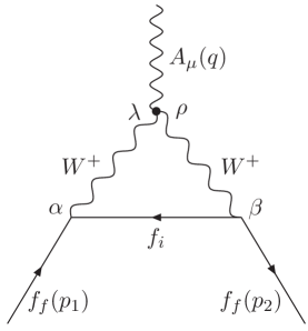
Figure 2: Contribution of the CP–odd $WW\gamma$ coupling to the on–shell $\bar{f}f\gamma$ vertex.

III.1 The $\tilde{{\cal O}}_{WB}$ contribution

We start with the contribution of the $\tilde{{\cal O}}_{WB}$ operator to the on–shell $\bar{f}f\gamma$ vertex. In the $R_{\xi}$–gauge, there are contributions coming from the $W$ boson and its associated pseudo Goldstone boson, but we prefer to use the unitary gauge in which the contribution is given only through the diagram shown in Fig.2. The corresponding amplitude is given by

$$\Gamma^{\tilde{{\cal O}}_{WB}}_{\mu}=\Bigg{(}\frac{e^{3}c_{W}}{4s^{3}_{W}}\tilde{\epsilon}_{WB}\Bigg{)}\epsilon_{\rho\lambda\mu\sigma}q^{\sigma}\mu^{4-D}\int\frac{d^{D}k}{(2\pi)^{D}}\frac{P_{R}\gamma_{\beta}\hbox{\large$/$}\kern-5.76042pt\hbox{$k$}\gamma_{\alpha}P^{\alpha\lambda}P^{\beta\rho}}{\Delta},$$ (24)

where

$$P^{\alpha\lambda} = g^{\alpha\lambda}-\frac{(k+p_{1})^{\alpha}(k+p_{1})^{\lambda}}{m^{2}_{W}},$$ (25)

$$P^{\beta\rho} = g^{\beta\rho}-\frac{(k+p_{2})^{\beta}(k+p_{2})^{\rho}}{m^{2}_{W}},$$ (26)

$$\Delta=[k^{2}-m^{2}_{i}][(k+p_{1})^{2}-m^{2}_{W}][(k+p_{2})^{2}-m^{2}_{W}].$$ (27)

The notation and conventions used in these expressions are shown in Fig.2. It is worth noting that the above amplitude is divergent, so the integral must be conveniently regularized in order to introduce a renormalization scheme. The authors of Ref.MQ introduced a cutoff by replacing $\tilde{\kappa}_{\gamma}$ with a form factor depending conveniently on the new physics scale $\Lambda$. Here, as already mentioned, we will regularize the divergencies using dimensional scheme. As far as the renormalization scheme is concerned, we will use the $\bar{MS}$ one with the renormalization scale $\mu=\Lambda$, which leads to a logarithmic dependence of the form $\log(\Lambda^{2}/m^{2}_{W})$. As we will see below, our procedure leads essentially to the same result given in Ref.MQ .

The fermionic EDM form factor $d_{f}$ is identified with the coefficient of the Lorentz tensor structure $-i\gamma_{5}\sigma_{\mu\nu}q^{\nu}$. The integrals that arise from the Feynman parametrization can be expressed in terms of elementary functions. After some algebra, one obtains

$$d^{\tilde{{\cal O}}_{WB}}_{f}=-\tilde{\epsilon}_{WB}\Big{(}\frac{\alpha c_{W}}{16\pi s^{3}_{W}}\Big{)}\Big{(}\frac{e}{2m_{W}}\Big{)}\sqrt{x_{f}}\Big{[}log\Big{(}\frac{m^{2}_{W}}{\Lambda^{2}}\Big{)}+f_{WB}(x_{f},x_{i})\Big{]},$$ (28)

where we have introduced the dimensionless variable $x_{a}=m^{2}_{a}/m^{2}_{W}$. Here, $f_{WB}(x_{f},x_{i})$ is the loop function, which is different for leptons or quarks. In the case of charged leptons, this function is given by

$$f_{WB}(x_{l})=-\frac{x_{l}+1}{x_{l}}+\frac{x^{2}_{l}-1}{x^{2}_{l}}\log(1-x_{l}),$$ (29)

where we have assumed that $x_{l}<1$. As far as the EDM of quarks is concerned, the $f_{WB}$ function has a more complicated way, given by

$$f_{WB}(x_{q},x_{i}) = -\frac{x_{q}+x_{i}+1}{x_{q}}+\frac{x^{2}_{q}+x^{2}_{i}-1}{2x^{2}_{q}}\log(x_{i})+$$ (30)

$$\frac{x^{3}_{q}-(x_{i}+1)x^{2}_{q}-(x_{i}+1)^{2}x_{q}+(x_{i}-1)^{2}(x_{i}+1)}{2x^{2}_{q}\lambda}f(x_{q},x_{i},\lambda),$$

where

$$f(x_{q},x_{i},\lambda)=\left\{\begin{array}[]{ll}\log\Big{(}\frac{x_{i}-x_{q}-\lambda+1}{x_{i}-x_{q}+\lambda+1}\Big{)},&\textrm{if \ \ $0<x_{q}<(1+\sqrt{x_{i}})^{2}$}\\ \log\Big{(}\frac{x_{i}-x_{q}-\lambda+1}{x_{i}-x_{q}+\lambda+1}\Big{)}-2i\pi,&\textrm{if $x_{q}>(1+\sqrt{x_{i}})^{2}$}\end{array}\right.,$$ (31)

with

$$\lambda=\sqrt{x^{2}_{q}-2(x_{i}+1)x_{q}+(x_{i}-1)^{2}}.$$ (32)

From now on, $m_{q}$ and $m_{i}$ will stand for the masses of the external and internal quarks, respectively.

III.2 The $\tilde{{\cal O}}_{W}$ contribution

We now turn to calculate the contribution of $\tilde{{\cal O}}_{W}$ to the fermion EDM. In this case, the contribution in the general $R_{\xi}$–gauge is given exclusively by the $W$ gauge boson through the diagram shown in Fig.2. Neither pseudo Goldstone bosons nor ghost fields can contribute, which is linked to the fact that, as noted previously, there are no contributions from the longitudinal components of the $W$ propagators due to the simple Ward identities given in Eq.(16). As a consequence, the result is manifestly gauge–independent, as any dependence on the $\xi$ gauge parameter disappears from the amplitude. Also, we have verified that $\tilde{{\cal O}}_{W}$ does not contribute to reducible diagrams characterized by the one–loop $Z-\gamma$ mixing. As already noted by the authors of Ref. MANYRS , the $\tilde{{\cal O}}_{W}$ operator, in contrast with the $\tilde{{\cal O}}_{WB}$ one, generates a finite contribution to $d^{\tilde{{\cal O}}_{W}}_{f}$.

As mentioned in the introduction, our result for this operator is in disagreement with that found in Ref.MANYRS . While the authors of this reference conclude that the loop function characterizing this contribution is of $O(1)$ in the low–energy limit (small fermions masses compared with $m_{W}$), we find that this function vanishes in this limit. As we will see below, this leads to a discrepancy of about two orders of magnitude for the bound on the $\tilde{\lambda}_{\gamma}$ parameter. It is therefore important to clarify this point as much as possible. For this purpose, let us to comment the main steps followed by the authors of Ref.MANYRS in obtaining their result. The starting point are Eqs.(2.11-2.13), which represent the amplitude for the contribution of the operator in consideration to the $\bar{f}f\gamma$ vertex. The next crucial step adopted by the authors consists in taking the photon momentum equal to zero both in the numerator and denominator of the integral given by Eq.(2.11), which leads to the simple expressions given in Eqs.(3.1,3.2). Next, they use dimensional regularization through Eqs.(3.5-3.11) to obtain the final result given by Eq.(3.12). This result comprises the sum of two terms, one which is independent of the masses involved in the amplitude, and a second term which vanishes in the low–energy limit. The first term arises from a careful treatment of the $D\to 4$ limit in dimensional regularization. We have reproduced all these results. However, we arrive at a very different result by using only the on–shell condition, so we think that it is not valid to delete the photon momentum before carrying out the integration on the momenta space. We now proceed to show that a different result is obtained if only the on–shell condition ($q^{2}=0$ and $q\cdot\epsilon$) is adopted. Our main result is that the loop function associated with this operator vanishes in the low–energy limit, in contrast with the result obtained in Ref.MANYRS . To be sure of our results, we will solve the momentum integral following two different methods, namely, the Passarino–Veltman PV covariant decomposition scheme and the Feynman parametrization technique. After using the Ward identities given in Eq.(16), the amplitude can be written as follows

$$\Gamma^{\tilde{{\cal O}}_{W}}_{\mu}=-\Big{(}\frac{e^{4}}{4!s^{3}_{W}m^{2}_{W}}\tilde{\epsilon}_{W}\Big{)}\int\frac{d^{D}k}{(2\pi)^{D}}\frac{P_{R}\gamma^{\rho}\hbox{\large$/$}\kern-5.76042pt\hbox{$k$}\gamma^{\lambda}\Gamma^{\tilde{\cal O}_{W}}_{\lambda\rho\mu}}{\Delta},$$ (33)

where $\Gamma^{\tilde{\cal O}_{W}}_{\lambda\rho\mu}$ represents the $WW\gamma$ vertex. Once carried out a Lorentz covariant decomposition, we implement the on–shell condition to obtain:

$$d^{\tilde{{\cal O}}_{W}}_{f} = -\tilde{\epsilon}_{W}\Big{(}\frac{\alpha^{3/2}}{32\sqrt{\pi}s^{3}_{W}}\Big{)}\Big{(}\frac{e}{2m_{W}}\Big{)}\frac{1}{\sqrt{x_{f}}}\Bigg{[}(x_{f}-1)\Big{(}B_{0}(1)-B_{0}(2)\Big{)}+2\Big{(}B_{0}(3)-B_{0}(1)\Big{)}$$ (34)

$$+x_{i}\Big{(}B_{0}(1)+B_{0}(2)-2B_{0}(3)\Big{)}+\Big{(}(x_{f}-x_{i})^{2}-1\Big{)}m^{2}_{W}C_{0}\Bigg{]},$$

where $B_{0}(1)=B_{0}(m^{2}_{f},m^{2}_{i},m^{2}_{W})$, $B_{0}(2)=B_{0}(0,m^{2}_{W},m^{2}_{W})$, $B_{0}(3)=B_{0}(0,m^{2}_{i},m^{2}_{W})$, and $C_{0}=C_{0}(m^{2}_{f},m^{2}_{f},0,m^{2}_{W},m^{2}_{i},m^{2}_{W})$ are Passarino–Veltman scalar functions. It is important to emphasize that in obtaining this result, the on–shell condition was implemented only after calculating the amplitude.

On the other hand, using Feynman parametrization, one obtains

$$d^{\tilde{{\cal O}}_{W}}_{f}=-\tilde{\epsilon}_{W}\Big{(}\frac{\alpha^{3/2}}{8\sqrt{\pi}s^{3}_{W}}\Big{)}\Big{(}\frac{e}{2m_{W}}\Big{)}\sqrt{x_{f}}(I_{1}+I_{2}+I_{3}),$$ (35)

where the $I_{i}$ quantities represent parametric integrals, which are given by

$$I_{1} = \int^{1}_{0}dxx(1-x)=\frac{1}{6},$$ (36)

$$I_{2} = -\int^{1}_{0}dx(1-x)(1-3x)\log[(1-x)(1-x_{f}x)+x_{i}x],$$ (37)

$$I_{3} = -x_{f}\int^{1}_{0}\frac{dxx^{2}(1-x)^{2}}{[(1-x)(1-x_{f}x)+x_{i}x]}.$$ (38)

To clarify our result, let us to analyze more closely these integrals. The $I_{1}$ integral, which is independent of the masses, arises as a residual effect of the $D\to 4$ limit. This apparent nondecoupling effect that would arise in the low–energy limit is also found in Ref.MANYRS . However, in our case, this effect is exactly cancelled at low energies by the $I_{2}$ integral, which in this limit takes the way:

$$I_{2}=-\frac{1}{6}+O(x_{f},x_{i}).$$ (39)

As for the $I_{3}$ integral, it vanishes in this limit. After solving the parametric integrals, one obtains

$$d^{\tilde{{\cal O}}_{W}}_{f}=-\tilde{\epsilon}_{W}\Big{(}\frac{\alpha^{3/2}}{16\sqrt{\pi}s^{3}_{W}}\Big{)}\Big{(}\frac{e}{2m_{W}}\Big{)}\sqrt{x_{f}}f_{W}(x_{f},x_{i}),$$ (40)

where $f_{W}(x_{f},x_{i})$ is the loop function. In the case of a charged lepton, this function is given by

$$f_{W}(x_{l})=\frac{x_{l}-2}{x_{l}}+2\Big{(}\frac{x_{l}-1}{x^{2}_{l}}\Big{)}\log(1-x_{l}).$$ (41)

On the other hand, the corresponding function for quarks is given by

$$f_{W}(x_{q},x_{i})=\frac{x_{q}-2}{x_{q}}+\frac{x_{q}+x_{i}-1}{x^{2}_{q}}\log(x_{i})+\frac{x^{2}_{q}-2x_{q}+(x_{i}-1)^{2}}{x^{2}_{q}\lambda}f(x_{q},x_{i},\lambda).$$ (42)

The same result is obtained when the Passarino–Veltman scalar functions appearing in Eq.(34) are expressed in terms of elementary functions.

In the light of the above results, we can conclude that it is not valid to delete the photon momentum before carrying out the integration on the momentum . In the next section, we will argue that a vanishing loop function in the low–energy limit is the result that one could expect in accordance with the decoupling theorem.

IV Results and discussion

We now turn to deriving bounds for the $\tilde{\epsilon}_{WB}$ and $\tilde{\epsilon}_{W}$ parameters (or equivalently, for the $\tilde{\kappa}_{\gamma}$ and $\tilde{\lambda}_{\gamma}$ parameters) using current experimental limits on the electron and the neutron electric dipole moments. We will use then these bounds to predict the CP–violating electromagnetic properties of the $W$ boson and some charged leptons and quarks.

One important advantage of our approach is that the effective Lagrangian respects the $SU_{L}(2)\times U_{Y}(1)$ symmetry. As a consequence, the coefficients of the $WW\gamma$ and $WWZ$ vertices are related at this dimension. The CP–violating part of this vertex is given by:

$${\cal L}_{WWZ}=-igc_{W}\Big{(}\tilde{\kappa}_{Z}W^{+}_{\mu}W^{-}_{\nu}\tilde{Z}^{\mu\nu}+\frac{\tilde{\lambda}_{Z}}{m^{2}_{W}}W^{+}_{\mu\nu}W^{-\nu}_{\ \ \rho}\tilde{Z}^{\rho\mu}\Big{)},$$ (43)

where $Z_{\mu\nu}=\partial_{\mu}Z_{\nu}-\partial_{\nu}Z_{\mu}$. The two set of parameters characterizing the $WW\gamma$ and $WWZ$ couplings are related by

$$\tilde{\kappa}_{Z} = -\frac{s^{2}_{W}}{c^{2}_{W}}\tilde{\kappa}_{\gamma},$$ (44)

$$\tilde{\lambda}_{Z} = \tilde{\lambda}_{\gamma}.$$ (45)

Below, we will constraint both sets of parameters.

The current experimental limits on the electric dipole moments of the electron and the neutron reported by the particle data book are PDG ; NB

$$|d_{e}|<6.9\times 10^{-28}\ \ \ e\cdot cm,$$ (46)

$$|d_{n}|<2.9\times 10^{-26}\ \ \ e\cdot cm.$$ (47)

IV.1 Decoupling and nondecoupling effects

Before deriving bounds on the $\tilde{\epsilon}_{WB}$ and $\tilde{\epsilon}_{W}$ parameters, let us discuss how radiative corrections can impact the four Lorentz tensor structures of the $WW\gamma$ vertex given by Eq.(1). Our objective is to clarify as much as possible why are so different the bounds that will be derived below for the $\tilde{\epsilon}_{WB}$ and $\tilde{\epsilon}_{W}$ coefficients. First of all, notice that both $F_{\mu\nu}W^{-\mu}W^{+\nu}$ and $\tilde{F}_{\mu\nu}W^{-\mu}W^{+\nu}$ terms have a renormalizable structure, as they are induced by the dimension–four invariants $W^{a}_{\mu\nu}W^{a\mu\nu}$ and $\tilde{W}^{a}_{\mu\nu}W^{a\mu\nu}$. However, in a perturbative context, only the former of these gauge invariants remains at the level of the classical action, as the latter can be written as a surface term. It turns out that, though renormalizable, the $\tilde{F}_{\mu\nu}W^{-\mu}W^{+\nu}$ interaction arises as a quantum fluctuation and thus it is naturally suppressed TT2 ; LRSM . The nondecoupling character of the $\Delta\kappa_{\gamma}$ and $\tilde{\kappa}_{\gamma}$ form factors is well–known from various specific models TT2 ; NDE . These Lorentz structures can in turn induce nondecoupling effects when inserted into a loop. In particular, they can impact significantly low–energy observables, as the EDM of light fermions. We will show below that this is indeed the case. In this context, it should be noticed the presence of the Higgs doublet in the $SU_{L}(2)\times U_{Y}(1)$–invariant operators of Eqs. (4,5), which points to a nontrivial link between the electroweak symmetry breaking scale and these couplings Iname . This connection is also evident in the nonlinear realization of the effective theory, in which the analogous of the operators (4) and (5) are:

$${\cal L}_{1} = a_{1}gg^{\prime}Tr\Big{(}U\frac{\sigma^{3}}{2}U^{\dagger}\frac{\sigma^{a}}{2}\Big{)}W^{a\mu\nu}B_{\mu\nu},$$ (48)

$$\tilde{{\cal L}}_{1} = a_{1}gg^{\prime}Tr\Big{(}U\frac{\sigma^{3}}{2}U^{\dagger}\frac{\sigma^{a}}{2}\Big{)}W^{a\mu\nu}\tilde{B}_{\mu\nu}.$$ (49)

Here, $U=exp\Big{(}\frac{i\sigma^{a}\phi^{a}}{v}\Big{)}$, with $\phi^{a}$ the would–be–Goldstone bosons MJH . Since in this model–independent parametrization the new physics is the responsible for the electroweak symmetry breaking, it is clear that such a link is beyond the Higgs mechanism. The situation is quite different for the $W^{+\mu}_{\nu}W^{-\lambda\nu}F_{\mu\lambda}$ and $W^{+\mu}_{\nu}W^{-\lambda\nu}\tilde{F}_{\mu\lambda}$ interactions, as they are nonrenormalizable and thus necessarily arise at one–loop or higher orders. The decoupling nature of these operators is also well–known TT2 ; NDE . It is important to notice that the Lorentz tensor structure of these terms is completely determined by the $SU_{L}(2)$ group and that there is no link with the electroweak symmetry breaking scale, in contrast with the $F_{\mu\nu}W^{-\mu}W^{+\nu}$ and $\tilde{F}_{\mu\nu}W^{-\mu}W^{+\nu}$ interactions. In this case, it is expected that loop effects of these operators decouples from low–energy observables. This fact has already been stressed by some authors DRujula . The reason why these interactions decouple from low–energy observables stems from the fact that the operators in Eqs.(6,7) respect a global $SU_{L}(2)$ custodial symmetry MANYRS . We will show below that the loop contributions of these operators to EDM is of decoupling nature.

We now turn to show the nondecoupling (decoupling) nature of the $\tilde{F}_{\mu\nu}W^{-\mu}W^{+\nu}$ ($W^{+\mu}_{\nu}W^{-\lambda\nu}\tilde{F}_{\mu\lambda}$) contribution to the EDM of light fermions. We will show that the $f_{WB}$ and $f_{W}$ loop functions have a very different behavior for small values of the fermion masses. We analyze separately the lepton and quark cases. For fermion masses small compared with the $W$ mass, we can expand the loop functions given by Eqs.(29,30) as follows:

$$f_{WB}(x_{l}) = -\frac{1}{2}-\frac{2}{3}x_{l}+\cdots,$$ (50)

$$f_{WB}(x_{q},x_{i}) = -\frac{1}{2}+2x_{i}-\frac{2}{3}x_{q}+\cdots$$ (51)

These results show clearly that the $\tilde{F}_{\mu\nu}W^{-\mu}W^{+\nu}$ term induces nondecoupling effects. In practice, this means that a good bound for the $\tilde{\kappa}_{\gamma}$ parameter could be derived still from experimental limits on the EDM of very light fermions, such as the electron. In contrast with this behavior, as already commented in the previous section, we can show that $f_{W}$ is of decoupling nature:

$$f_{W}(x_{l}) = -\frac{1}{3}x_{l}+\cdots,$$ (52)

$$f_{W}(x_{q},x_{i}) = x_{i}-\frac{1}{3}x_{q}+\cdots$$ (53)

This means that the $\tilde{{\cal O}}_{W}$ operator only could lead to significant contributions for heavier fermions. We will show below that the bound obtained for $\tilde{\lambda}_{\gamma}$ from the experimental limit on the EDM of the electron differs in $9$ orders of magnitude with respect to that obtained from the corresponding limit of the neutron, whereas in the case of the $\tilde{\kappa}_{\gamma}$ parameter the analogous bounds differ in less than 2 orders of magnitude. The high sensitivity of the $f_{W}$ function to the mass ratios $m_{f}/m_{W}$ and $m_{i}/m_{W}$ is shown in Table 1. It is interesting to see that $f_{W}$ and $f_{WB}$ differ in 4 orders of magnitude for a fermion mass of about a third of the neutron mass, though they differ in 10 orders of magnitude for the case of the electron mass. Moreover, notice that $f_{WB}$ and $f_{W}$ are of the same order of magnitude for the third quark family. This means that the $\tilde{{\cal O}}_{W}$ operator might play an important role in top quark physics. The very different behavior of the loop functions in the lepton and quark sectors can be appreciated in Table 1. Also, it should be mentioned that the loop functions develop an imaginary part in the case of an external quark top. The appearance of an imaginary (absorptive) part is a consequence of the fact that the external mass is larger than the sum of the two internal masses: $m_{t}>m_{W}+m_{b}$.

Table 1: Behavior of the $f_{WB}$ and $f_{W}$ loop functions for some specific values of the internal ($m_{i}$) and external ($m_{f}$) fermion masses.

$m_{f}$	$m_{i}$	$x_{f}$	$x_{i}$	$f_{WB}(x_{f},x_{i})$	$f_{W}(x_{f},x_{i})$
$e$	$\nu_{e}$	$3.9\times 10^{-11}$	$0$	$-0.50$	$-1.3\times 10^{-11}$
$\mu$	$\nu_{\mu}$	$1.6\times 10^{-6}$	$0$	$-0.50$	$-5.2\times 10^{-7}$
$\tau$	$\nu_{\tau}$	$5.0\times 10^{-4}$	$0$	$-0.50$	$-1.6\times 10^{-4}$
$m_{n}/3$	$m_{n}/3$	$1.5\times 10^{-5}$	$1.5\times 10^{-5}$	$-0.49$	$+1.0\times 10^{-5}$
$s$	$c$	$2.3\times 10^{-6}$	$2.6\times 10^{-4}$	$-0.49$	$+2.4\times 10^{-4}$
$c$	$s$	$2.6\times 10^{-4}$	$2.3\times 10^{-6}$	$-0.50$	$+7.9\times 10^{-5}$
$b$	$t$	$2.8\times 10^{-3}$	$4.7$	$+1.30$	$+0.6$
$t$	$b$	$4.7$	$2.8\times 10^{-3}$	$4.7\times 10^{-2}-3i$	$1.02-1.05i$

IV.2 Bounding the $\tilde{{\cal O}}_{WB}$ operator

We now turn to deriving a bound for the $\tilde{\kappa}_{\gamma}$ coefficient using the current experimental limit on the EDM of the electron and the neutron. In the case of the electron EDM, we can approximate the $f_{WB}(x_{e})$ loop function as follows:

$$f_{WB}(x_{e})\approx-\frac{1}{2}-\frac{1}{2}x_{e}.$$ (54)

Using this approximation, Eqs. (28) and (46) lead to

$$\Bigg{|}\tilde{\epsilon}_{WB}\Bigg{(}\log\Big{(}\frac{\Lambda^{2}}{m^{2}_{W}}\Big{)}+\frac{1}{2}+\frac{1}{2}x_{e}\Bigg{)}\Bigg{|}<1.3\times 10^{-4}.$$ (55)

Since in the effective Lagrangian approach one assumes that $\Lambda\gg m_{W}$, it is clear that

$$log\Big{(}\frac{\Lambda^{2}}{m^{2}_{W}}\Big{)}+\frac{1}{2}+\frac{1}{2}x_{e}>1,$$ (56)

which allows us to impose the following bound on the ${\cal O}_{WB}$ operator

$$|\tilde{\epsilon}_{WB}|<1.6\times 10^{-3},$$ (57)

which in turn leads to

$$|\tilde{\kappa}_{\gamma}|<1.5\times 10^{-3},\ \ \ |\tilde{\kappa}_{Z}|<4.2\times 10^{-4}.$$ (58)

In the case of the neutron, as usual, we take $m_{u}\approx m_{d}\approx m_{n}/3$, with $m_{n}$ the neutron mass. Also, we assume the following relation:

$$d_{n}=\frac{4}{3}d_{d}-\frac{1}{3}d_{u}.$$ (59)

Using this connection between the neutron and its constituents, one obtains for the $\tilde{{\cal O}}_{WB}$ contribution to the neutron EDM

$$d^{{\tilde{\cal O}}_{WB}}_{n}=\tilde{\epsilon}_{WB}\Big{(}\frac{\alpha c_{W}}{48\pi s^{3}_{W}}\Big{)}\Big{(}\frac{e}{2m_{W}}\Big{)}\sqrt{x_{n}}\Big{[}\log\Big{(}\frac{\Lambda^{2}}{m^{2}_{W}}\Big{)}+f_{WB}(x_{n})\Big{]},$$ (60)

where

$$f_{WB}(x_{n})=2+\frac{9}{x_{n}}+\frac{81-2x^{2}_{n}}{x^{2}_{n}}log\Big{(}\frac{x_{n}}{9}\Big{)}+\frac{4x^{2}_{n}+18x_{n}-81}{2x^{2}_{n}\lambda_{n}}\log\left(\frac{1-\lambda_{n}}{1+\lambda_{n}}\right),$$ (61)

with $\lambda_{n}=\sqrt{9-4x_{n}}/3$. Comparing the above theoretical result with its experimental counterpart given by Eq.(47), one obtains

$$\Bigg{|}\tilde{\epsilon}_{WB}\Bigg{(}\log\Big{(}\frac{\Lambda^{2}}{m^{2}_{W}}\Big{)}+f_{WB}(x_{n})\Bigg{)}\Bigg{|}<5.5\times 10^{-5}.$$ (62)

As in the electron case, it is easy to see that

$$\Bigg{|}\log\Big{(}\frac{\Lambda^{2}}{m^{2}_{W}}\Big{)}+f_{WB}(x_{n})\Bigg{|}>1,$$ (63)

which allows us to impose the following bound on the $\tilde{{\cal O}}_{WB}$ operator

$$|\tilde{\epsilon}_{WB}|<5.5\times 10^{-5},$$ (64)

which implies

$$|\tilde{\kappa}_{\gamma}|<5.2\times 10^{-5},\ \ \ |\tilde{\kappa}_{Z}|<1.5\times 10^{-5}.$$ (65)

This bound is almost two orders of magnitude more stringent than that obtained from the electron EDM. The above results are in perfect agreement with the ones given in Ref.MQ .

IV.3 Bounding the $\tilde{{\cal O}}_{W}$ operator

We first explore the possibility of constraining $\tilde{{\cal O}}_{W}$ using the experimental limit on the electron EDM. In this case, a good approximation for the loop function is $f_{W}(x_{e})\approx-x_{e}\sim-3\cdot 9\times 10^{-11}$, which in fact is very small. It leads to a very poor constrain of order of $10^{7}$. This bound should be compared with the one obtained in Ref.MANYRS , which can be updated to $|\tilde{\lambda}_{\gamma}|<7\times 10^{-4}$. This enormous difference arises because the authors in Ref.MANYRS assume that $f_{W}\sim O(1)$, instead of $f_{W}(x_{e})\approx-x_{e}\sim-3.9\times 10^{-11}$.

We now try to get a more restrictive bound from the experimental limit on the neutron EDM. Following the same steps given above, the connection between the EDM of the neutron with its constituents given in Eq.(59) leads to

$$d^{\tilde{{\cal O}}_{W}}_{n}=-\tilde{\epsilon}_{W}\Big{(}\frac{\alpha^{3/2}}{48\sqrt{\pi}s^{2}_{W}}\Big{)}\Big{(}\frac{e}{2m_{W}}\Big{)}\sqrt{x_{n}}f_{W}(x_{n}),$$ (66)

where

$$f_{W}(x_{n})=2\Big{(}1-\frac{9}{x_{n}}\Big{)}+\frac{9(2x_{n}-9)}{x^{2}_{n}}\log\Big{(}\frac{x_{n}}{9}\Big{)}+\frac{2x^{2}_{n}-36x_{n}+81}{x^{2}_{n}\lambda_{n}}\log\left(\frac{1-\lambda_{n}}{1+\lambda_{n}}\right).$$ (67)

In this case a more restrictive bound is obtained:

$$|\tilde{\epsilon}_{W}|<0.12,$$ (68)

which in turn leads to

$$|\tilde{\lambda}_{\gamma}|=|\tilde{\lambda}_{Z}|<1.9\times 10^{-2}.$$ (69)

In this case the result obtained in Ref.MANYRS can be updated to $|\tilde{\lambda}_{\gamma}|<6\times 10^{-5}$, which shows that our constraint is less stringent by more than 2 orders of magnitude.

From the above results, the high sensitivity of the $(\tilde{\lambda}_{\gamma}/m^{2}_{W})W^{+}_{\mu\nu}W^{-\nu}_{\ \ \rho}\tilde{F}^{\rho\mu}$ interaction to the mass ratio $m_{f}/m_{W}$ can be appreciated now.

IV.4 CP–odd electromagnetic properties of fermions and the $W$ gauge boson

The constraints derived above for the CP–odd $WW\gamma$ vertex can be used to predict the CP–odd electromagnetic properties of known particles. In particular, the EDM associated with the heavier particles are the most interesting, as they could be more sensitive to new physics effects. Besides the $W$ gauge boson and the third family of leptons and quarks, we will also include by completeness the predictions on the members of the second family. In the case of the $W$ gauge boson, an upper bound for the magnetic quadrupole moment will also be presented. It should be emphasized the fact that it is the first time that an upper bound on $\tilde{Q}_{W}$ is derived. We will use the constraints derived from the neutron EDM, as they are most stringent. Since the $\tilde{{\cal O}}_{WB}$ and $\tilde{{\cal O}}_{W}$ operators were bounded one at a time, we will make predictions assuming that the CP–violating effects cannot arise simultaneously from both operators. We resume our results in Table 2. It should be noted that while the values for $d_{W}$ and $\tilde{Q}_{W}$ constitute true upper bounds, the ones given by the EDM of fermions are estimations only.

Table 2: Electromagnetic properties of the known particles induced by a CP–violating $WW\gamma$ vertex. The value $\Lambda=1000$ GeV is assumed for the contribution of the $\tilde{{\cal O}}_{WB}$ operator.

Particle	Electric Dipole Moment	$\tilde{{\cal O}}_{WB}$	$\tilde{{\cal O}}_{W}$
$\mu$	$|d_{\mu}|$	$5.7\times 10^{-26}\ e\cdot cm$	$2.0\times 10^{-30}\ e\cdot cm$
$\tau$	$|d_{\tau}|$	$1.0\times 10^{-24}\ e\cdot cm$	$1.1\times 10^{-26}\ e\cdot cm$
$c$	$|d_{c}|$	$7.1\times 10^{-25}\ e\cdot cm$	$3.8\times 10^{-27}\ e\cdot cm$
$s$	$|d_{s}|$	$6.5\times 10^{-26}\ e\cdot cm$	$1.0\times 10^{-27}\ e\cdot cm$
$b$	$|d_{b}|$	$2.1\times 10^{-21}\ e\cdot cm$	$9.9\times 10^{-23}\ e\cdot cm$
$t$	$|Re(d_{t})|$	$1.6\times 10^{-22}\ e\cdot cm$	$6.8\times 10^{-21}\ e\cdot cm$
$t$	$|Im(d_{t})|$	$6.0\times 10^{-23}\ e\cdot cm$	$7.0\times 10^{-21}\ e\cdot cm$
$W$	$|d_{W}|$	$6.2\times 10^{-21}\ e\cdot cm$	$2.3\times 10^{-18}\ e\cdot cm$
$W$	$|\tilde{Q}_{W}|$	$3.0\times 10^{-36}\ e\cdot cm^{2}$	$1.1\times 10^{-33}\ e\cdot cm^{2}$

It is worth comparing the limits given in Table 2 with some predictions obtained in other contexts. We begin with the results existing in the literature for the $W$ gauge boson. We start with the SM predictions for $d_{W}$ and $\tilde{Q}_{W}$. As already mentioned, the lowest order nonzero contribution to $d_{W}$ arises at the three–loop level, whereas $\tilde{Q}_{W}$ appears up to the two–loop order. At the lowest order, $d_{W}$ has been estimated to be smaller than about $10^{-29}\ e\cdot cm$ EDMQW2 ; PP . As far as $\tilde{Q}_{W}$ is concerned, it has been estimated to be about $-10^{-51}\ e\cdot cm^{2}$ MQMW . Beyond the SM, almost all studies have focused on $d_{W}$. Results several orders of magnitude larger than the SM prediction have been found. For instance, a value of $10^{-22}\ e\cdot cm$ was estimated for $d_{W}$ in left–right symmetric models EDMQW2 ; LRSM and also in supersymmetric models EDMQW2 ; NC . Also, a nonzero $d_{W}$ can arise through two–loop graphs in multi–Higgs models SW . Explicit calculations carried out within the context of the two–Higgs doublet model (THDM) show that $d_{W}\sim 10^{-21}\ e\cdot cm$ THDM . A similar value was found within the context of the so–called 331 models 331 . Recently, the one–loop contribution of a CP–violating $HWW$ vertex to both $d_{W}$ and $\tilde{Q}_{W}$ was studied in the context of the effective Lagrangian approach TT1 . By assuming reasonable values for the unknown parameters, it was found that $d_{W}\sim 3-6\times 10^{-21}\ e\cdot cm$ and $\tilde{Q}_{W}\sim-10^{-36}\ e\cdot cm^{2}$, which are 8 and 15 orders of magnitude above the SM contribution. More recently, the one–loop contribution of the anomalous $tbW$ vertex, which includes both left– and right–handed complex components, to $d_{W}$ and $\tilde{Q}_{W}$ was calculated HHPTT . By using the most recent bounds on the $tbW$ coupling from $B$ meson physics, it was estimated that $d_{W}\sim 4\times 10^{-23}-4\times 10^{-22}\ e.cm$ and $\tilde{Q}_{W}\sim 10^{-38}-10^{-37}\ e.cm^{2}$. All these predictions for $d_{W}$ and $\tilde{Q}_{W}$ are consistent with the upper bounds given in Table 2.

We now proceed to compare the predictions for the EDM of leptons and quarks given in Table 2 with results obtained in some specific models. As already noted, the values reported for the EDM of fermions are not upper bounds, as in the case of the $W$ boson, but only estimates for these quantities, since they are derived by assuming that CP–violation is induced via a CP–odd $WW\gamma$ vertex. However, it is clear that others sources of CP–violation could eventually lead to values larger than those presented here. They are however illustrative of the sensitivity of fermions to CP–odd effects, so we believe that these results deserve a wider discussion still in this somewhat restricted scenario. First, we would like to discuss the prediction existing in the literature for the $\mu$ and $\tau$ leptons. In the case of the muon, the Particle Data Group PDG reports an experimental limit of about $d_{\mu}<10^{-19}\ e\cdot cm$. As far as theoretical predictions are concerned, the SM prediction is about $10^{-35}\ e\cdot cm$, which is 16 orders of magnitude below the experimental limit. This means that precise measurements of the muon EDM might reveal new sources of CP violation. Although very suppressed in the SM, some of its extensions predicts values for $d_{\mu}$ that are several orders of magnitude larger. For instance, an estimate of $10^{-24}\ e\cdot cm$ for $d_{\mu}$ was obtained in the THDM MTHDM . Similar results have been found within the context of supersymmetric models MSUSY and in the presence of large neutrino mixing MNM . SUSY model also predict large lepton EDMs if there are many right-handed neutrinos along with large values of $tan\beta$ E . A wider variety of theoretical perspectives are studied in MTP , where it is found that $d_{\mu}$ can be as large as $10^{-22}\ e\cdot cm$. This value is approximately 4 and 8 orders of magnitude above than those induced by the $\tilde{{\cal O}}_{WB}$ and $\tilde{{\cal O}}_{W}$ operators, respectively. As far as the the tau lepton is concerned, the experimental limit is $-0.22\times 10^{-16}\ e\cdot cm<Re(d_{\tau})<0.45\times 10^{-16}\ e\cdot cm$ PDG . Since this lepton has a relatively high mass and a very short lifetime, it is expected that its dynamics is more sensitive to physics beyond the Fermi scale. Indirect bounds of order of $|d_{\tau}|<O(10^{-17})\ e\cdot cm$ have been obtained from precision LEP data ESCRIBANO and naturalness arguments PRL . Some model independent analysis predict possible values of order $|d_{\tau}|\sim 10^{-19}\ e\cdot cm$ due to new physics effects. The possible measurement of $d_{\tau}$ at low energy experiments is analyzed in B . All these predictions are consistent with the experimental limit, but are above by at least 7 orders of magnitude with respect to our estimation that arises from a CP–odd $WW\gamma$ vertex. As far as the EDM of quarks is concerned, most studies have been focused on the third family. In the literature, the EDM of the $b$ and $t$ quarks has been calculated in many variants of multi–Higgs models MHM , as it is expected that more complicated Higgs sectors tend to favor this class of new physics effects. The dipole moments were estimated to be of order of $d_{b}\sim 10^{-23}-10^{-22}\ e\cdot cm$ and $d_{t}\sim 10^{-21}-10^{-20}\ e\cdot cm$. Very recently, an estimate for $d_{t}$ of about $10^{-22}\ e\cdot cm$ was obtained from the one–loop contribution of an anomalous $tbW$ vertex that includes both left– and right–handed complex components HHPTT . It is interesting to see that in this case the predictions are quite similar to our estimations derived from the CP–odd $WW\gamma$ vertex. Also, notice that $\tilde{{\cal O}}_{W}$ induces the most important contribution.

V Conclusions

The origin of CP violation has remained an unsolved problem since its discovery several decades ago. Even if the CKM matrix is the correct mechanism to describe CP violation in $K$ and $B$ meson systems, this is not necessarily the only source of CP violation in the nature. Non–zero electric dipole moments of elementary particles would be a clear evidence of the presence of new sources of CP violation. In this paper, a source of CP violation mediated by the $WW\gamma$ vertex has been analyzed using the effective Lagrangian technique and its implications on the CP–odd electromagnetic properties of the SM particles studied. Two dimension–six $SU_{L}(2)\times U_{Y}(1)$– invariant operators, $\tilde{{\cal O}}_{WB}$ and $\tilde{{\cal O}}_{W}$, which reproduce the two independent Lorentz tensor structures, $\tilde{\kappa}_{\gamma}W^{+}_{\mu}W^{-}_{\nu}\tilde{F}^{\mu\nu}$ and $(\tilde{\lambda}_{\gamma}/m^{2}_{W})W^{+}_{\mu\nu}W^{-\nu}_{\ \ \rho}\tilde{F}^{\rho\mu}$, that determine the electric dipole, $d_{W}(\tilde{\kappa}_{\gamma},\tilde{\lambda}_{\gamma})$, and magnetic quadrupole, $\tilde{Q}_{W}(\tilde{\kappa}_{\gamma},\tilde{\lambda}_{\gamma})$, moments of the $W$ gauge boson, were introduced. The contribution of this vertex to the EDM of charged leptons and quarks was calculated. The main features of these operators were studied in detail. One interesting peculiarity of the $\tilde{{\cal O}}_{W}$ operator consists in the fact that it generates a $WW\gamma$ vertex that satisfies simple Ward identities. As a direct consequence, the contribution of this vertex in any multi–loop amplitude is manifestly gauge–independent. As pointed out by other authors, it was found that while $\tilde{{\cal O}}_{WB}$ leads to a divergent amplitude for the fermion EDM, the $\tilde{{\cal O}}_{W}$ contribution is free of ultraviolet divergences. The low–energy behavior of these operators was analyzed in the light of the decoupling theorem. We emphasized the important fact that while the $\tilde{{\cal O}}_{WB}$ operator is strongly linked with the electroweak symmetry breaking (whatever it origin may be), the $\tilde{{\cal O}}_{W}$ one has not connection with the electroweak scale. As a consequence, the former does not decouple at low energies, whereas the latter has a decoupling nature. Owing to this fact, there is a difference of more than two orders of magnitude in the respective bounds obtained from low energy data, in contradiction with previous results given in the literature where constraints of the same order of magnitude were derived. The origin of such a disagreement was discussed. At high energies, the contributions of these operators are equally important. However, since $\tilde{{\cal O}}_{W}$ is weakly constrained by low energy experiments, it might have an important impact on CP violating observables at high energy collisions. Due to this fact, $\tilde{{\cal O}}_{W}$ might be more promising than $\tilde{{\cal O}}_{WB}$ in searching CP violating effects at high energy experiments. In order to appreciate these peculiarities, the behavior of the corresponding loop amplitudes were studied in detail. The experimental limits on the neutron and electron EDM were used to get bounds on the $\tilde{\kappa}_{\gamma}$ and $\tilde{\lambda}_{\gamma}$ parameters. It was found that the best constraints arise from the experimental limit on the neutron EDM, which leads to $|\tilde{\kappa}_{\gamma}|<5.2\times 10^{-5}$ and $|\tilde{\lambda}_{\gamma}|<1.9\times 10^{-2}$. The former limit implies the upper bounds $|d_{W}(5.2\times 10^{-5},0)|<6.2\times 10^{-21}\ e\cdot cm$, $|\tilde{Q}_{W}(5.2\times 10^{-5},0)|<3.0\times 10^{-36}\ e\cdot cm^{2}$, whereas the latter leads to $|d_{W}(0,1.9\times 10^{-2})|<2.3\times 10^{-18}\ e\cdot cm$, and $|\tilde{Q}_{W}(0,1.9\times 10^{-2})|<1.1\times 10^{-33}\ e\cdot cm^{2}$. As far as the limit on $\tilde{\kappa}_{\gamma}$ and the upper bound on $d_{W}$ are concerned, we found agrement with the results obtained by Marciano and Queijeiro MQ . The $SU_{L}(2)\times U_{Y}(1)$ invariance of our approach was exploited to impose constraints on the $\tilde{\kappa}_{Z}$ and $\tilde{\lambda}_{Z}$ parameters associated with the weak coupling $WWZ$. It was found that $|\tilde{\kappa}_{Z}|<1.5\times 10^{-5}$ and $|\tilde{\lambda}_{Z}|<1.9\times 10^{-2}$. The limits on the $\tilde{\kappa}_{\gamma}$ and $\tilde{\lambda}_{\gamma}$ parameters were used to estimate the EDM of the muon and tau leptons, as well as the bottom and top quarks. In the lepton case, we estimated $d_{\mu}\sim 10^{-26}-10^{-30}\ e\cdot cm$ and $d_{\tau}\sim 10^{-22}-10^{-26}\ e\cdot cm$, which are 4 and 5 orders of magnitude below than estimates obtained in other models, respectively. In the case of the $b$ and $t$ quarks, our estimate is $d_{b}\sim 10^{-21}-10^{-24}\ e\cdot cm$ and $d_{t}\sim 10^{-20}-10^{-22}\ e\cdot cm$, which are of the same order of magnitude than some results found in other contexts. In general terms, our results indicate that the heavier fermions, as the $b$ and $t$ quarks, tend to be more sensitive to new sources of CP violation.

- (1) For a recent review, see M. Pospelov and A. Ritz, Ann. Phys. (N.Y.) 318, 119 (2005).
- (2) M. E. Pospelov and I. B. Khriplovich, Sov. J. Nucl. Phys. 53, 638 (1991) [Yad. Fiz. 53, 1030 (1991)]; E. P. Shabalin, Sov. J. Nucl. Phys. 28, 75 (1978) [Yad. Fiz. 28, 151 (1978)].
- (3) D. Chang, W. Y. Keung, and J. Liu, Nucl. Phys. B355, 295 (1991).
- (4) I. B. Khriplovich and M. E. Pospelov, Nucl. Phys. B420, 505 (1994).
- (5) J. Montao, F. Ramírez–Zavaleta, G. Tavares–Velasco, and J. J. Toscano, Phys. Rev. D72, 115009 (2005).
- (6) J. Hernández–Sánchez, C. G. Honorato, F. Procopio, G. Tavares–Velasco, and J. J. Toscano, Phys. Rev. D75, 073017 (2007).
- (7) S. M. Barr and W. J. Marciano, in CP Violation, edited by C. Jarlskog (World Scientific, Singapoire, 1989).
- (8) W. J. Marciano and A. Queijeiro, Phys. Rev. D33, 3449 (1986).
- (9) G. Tavares–Velasco and J. J. Toscano, J. Phys. G30, 1299 (2004).
- (10) D. Atwood, C. P. Burgess, C. Hamazaou, B. Irwin, and J. A. Robinson, Phys. Rev. D42, 3770 (1990).
- (11) W. Buchmuller and D. Wyler, Nucl. Phys. B268, 621 (1986).
- (12) K. Hagiwara, R. D. Peccei, D. Zeppenfeld, and K. Hikasa, Nucl. Phys. B282, 253 (1987).
- (13) For a review, see J. Ellison and J. Wudka, Ann. Rev. Nucl. Part. Sci. 48, 33 (1998).
- (14) A. Grau and J. A. Grifols, Phys. Lett. B154, 283 (1985); J. C. Wallet, Phys. Rev. D32, 813 (1985); P. Merry, S. E. Moubarik, M. Perrottet, and F. M. Renard, Z. Phys. C46, 229 (1990); F. Hoogeveen, Max–Planck–Institut Report No. MPI-PAE/PTh 25/87, 1987 (unpublished); F. Boudjema, C. P. Burgess, C. Hamzaoui, and J. A. Robinson, Phys. Rev. D43, 3683 (1991); C. P. Burgess, M. Frank, and C. Hamzaoui, Z. Phys. C70, 145 (1996).
- (15) F. Boudjema, K. Hagiwara, C. Hamzaoui, and K. Numata, Phys. Rev. D43, 2223 (1991).
- (16) C. Arzt, M. B. Einhorn, and J. Wudka, Phys. Rev. D49, 1370 (1994).
- (17) T. Appelquist and J. Carazzone, Phys. Rev. D11, 2856 (1975).
- (18) See for instance, J. Wudka, Int. J. Mod. Phys. A9, 2301 (1994).
- (19) See for instance, M. A. Pérez and J. J. Toscano, Phys. Lett. B289, 381 (1992); K. Hagiwara, S. Ishihara, R. Szalapski, and D. Zeppenfeld, Phys. Rev. D48, 2182 (1993); M. A. Pérez, J. J. Toscano, and J. Wudka, Phys. Rev. D52, 494 (1995); J. L. Díaz–Cruz, J. Hernández–Sánchez, and J. J. Toscano, Phys. Lett. B512, 339 (2001).
- (20) G. Passarino and M. J. G. Veltman, Nucl. Phys. B160, 151 (1979).
- (21) See for instance, G. Tavares–Velasco and J. J. Toscano, Phys. Rev. D65, 013005 (2001).
- (22) W. -M. Yao, et al. (Particle Data Group), J. Phys. G33, 1 (2006).
- (23) The most recent bound on the neutron electric dipole moment is reported in: C. Baker et al., Phys. Rev. Lett. 97, 131801 (2006).
- (24) W. A. Bardeen, R. Gastmans, and B. Lautrup, Nucl. Phys. B46, 319 (1972); G. Couture and J. N. Ng, Z. Phys. C35, 65 (1987); G. Couture, J. N. Ng, J. L. Hewett, and T. G. Rizzo, Phys. Rev. D36, 859 (1987); C. L. Bilachak, R. Gatsmans, and A. van Proeyen, Nucl. Phys. B273, 46 (1986); G. Couture, J. N. Ng, J. L. Hewett, and T. G. Rizzo, Phys. Rev. D38, 860 (1988); A. B. Lahanas and V. C. Sapanos, Phys. Lett. B334, 378 (1994); T. M. Aliyev, ibid., 155, 364 (1985); A. Arhrib, J. L. Kneur, and G. Moultaka, ibid., 376, 127 (1996); N. K. sharma, P. Saxena, Sardar Singh, A. K. Nagawat, and R. S. Sahu, Phys. Rev. D56, 4152 (1997); T. G. Rizzo and M. A. Samuel, Phys. Rev. D35, 403 (1987); A. J. Davies, G. C. Joshi, and R. R. Volkas, ibid., 42, 3226 (1990); F. Larios, J. A. Leyva, and R. Martínez, Phys. Rev. D53, 6686 (1996); G. Tavares–Velasco and J. J. Toscano, Phys. Rev. D69, 017701 (2004); J. L. García–Luna, G. Tavares–Velasco, and J. J. Toscano, Phys. Rev. D69, 093005 (2004); J. Monta o, F. Ramírez–Zavaleta, G. Tavares–Velasco, and J. J. Toscano, Phys. Rev. D72, 055023 (2005); F. Ramírez–Zavaleta, G. Tavares–Velasco, and J. J. Toscano, Phys. Rev. D75, 075008 (2007).
- (25) T. Inami, C. S. Lim, B. Takeuchi, and M. Tanabashi, Phys. Lett. B381, 458 (1996).
- (26) For an introduction to Electroweak Chiral Lagrangians, see Mar ía José Herrero, hep-ph/9601286.
- (27) A. De Rújula, M. B. Gavela, O. Pene, and F. J. Vegas, Nucl. Phys. B357, 311 (1991); A. De Rújula, M. B. Gavela, P. Hernández, and E. Masso, Nucl. Phys. B384, 3 (1992).
- (28) M. J. Booth, hep-ph/9301293.
- (29) I. Vendramin, Nuovo Cimento Soc. Ital. Fis. A 105, 1649 (1992); T. H. West, Phys. Rev. D50, 7025 (1994); T. Kadoyoshi and N. Oshimo, Phys. Rev. D55, 1481 (1997); N. Oshimo, Nucl. Phys. B, Proc. Suppl. 59, 231 (1997).
- (30) S. Weinberg, Phys. Rev. D42, 860 (1990).
- (31) R. Lopez–Mobilia and T. H. West, Phys. Rev. D51, 6495 (1995); I. Vendramin, Nuovo Cimento Soc. Ital. Fis. A 106, 79 (1993).
- (32) C. S. Huang and T. J. Li, Phys. Rev. D50, 2127 (1994).
- (33) V. Barger, A. Das, and C. Kao, Phys. Rev. D55, 7099 (1997).
- (34) T. Ibrahim and P. Nath, Phys. Rev. D64, 093002 (2001).
- (35) K. S. Babu, B. Dutta, and R. Mohapatra, Phys. REv. Lett. 85, 5064 (2000).
- (36) J. R. Ellis and O. Lebedev, Phys. Lett.B653, 411 (2007); arXiv:0707.4319.
- (37) J. L. Feng, K. T. Matchev, and Y. Shadmi, Nucl. Phys. B613, 366 (2001).
- (38) R. Escribano and E. Massó, Phys. Lett. B301, 419 (1993); Nucl. Phys. B429, 19 (1994); Phys. Lett. B395, 369 (1997).
- (39) K. Akama, T. Hattori, and K. Katsuura, Phys. Rev. Lett. 88, 201601 (2002).
- (40) J. Bernabéu, G. A. González–Sprinberg, and J. Vidal, Nucl. Phys. B763, 283 (2007).
- (41) S. Weinberg, Phys. Rev. Lett. 58, 657 (1976); G. C. Branco and M. N. Robelo, Phys. Lett. B160, 117 (1985); J. Liu and L. Wolfenstein, Nucl. Phys. B289, 1 (1987); C. H. Albright, J. Smith, and S. H. H. Tye, Phys. Rev. D21, 711 (1980); A. Soni and R. M. Xu, Phys. Rev. Lett. 69, 33 (1992); N. G. Deshpande and E. Ma, Phys. Rev. D16, 1583 (1977); Y. Liao and X. Li, Phys. Rev. D60, 073004 (1999); D. G. Dumm and G. A. Sprinberg, Eur. Phys. J. C11, 293 (1999); D. A. Demir and M. B. Voloshin, Phys. Rev. D63, 115011 (2001); E. O. Iltan, J. Phys. G27, 1723 (2001); Phys. Rev. D65, 073013 (2002).