The matrix product representations for all valence bond states
         Vahid Karimipour ,         Laleh Memarzadeh,

Department of Physics, Sharif University of Technology,

P.O. Box 11155-9161, Tehran, Iran

We introduce a simple representation for irreducible spherical tensor operators of the rotation group of arbitrary integer or half integer rank and use these tensor operators to construct matrix product states corresponding to all the variety of valence-bond states proposed in the Affleck-Kennedy-Lieb-Tasaki (AKLT) construction. These include the fully dimerized states of arbitrary spins, with uniform or alternating patterns of spins, which are ground states of Hamiltonians with nearest and next-nearest neighbor interactions, and the partially dimerized or AKLT/VBS (Valence Bond Solid) states, which are constructed from them by projection. The latter states are translation-invariant ground states of Hamiltonians with nearest-neighbor interactions.

PACS: 03.67.-a, 75.10 Jm.

1 Introduction

The problem of introducing exactly solvable models in quantum spin chains has a long history in statistical mechanics and mathematical physics, which encompasses a variety of models and techniques [1, 2]. One can mention the $XY$ [3], the Heisenberg $XXX$ and $XXZ$ [4], the AKLT [5], and the Majumdar-Ghosh models [6], and the free fermion, the Bethe ansatz, and the matrix product techniques to name only a few of the most important models and techniques which have been developed so far. Finding any new exactly solvable model, is an important step, since it acts as a reference model for developing approximate perturbative solutions for more realistic models. It will also help us to test many of the new ideas about collective behavior of quantum systems, i.e. entanglement properties [7, 8], or the relation of criticality and universality of entanglement [9, 10].

In [5], Affleck, Kennedy, Lieb and Tasaki (AKLT), suggested a new construction for a variety of spin states, known as valence bond states. The basic element of this construction is a spin-1/2 singlet state, a dimer, $|s\rangle=\frac{1}{\sqrt{2}}(|+,-\rangle-|-,+\rangle)$ which is called a valence bond in [5]. A dimerized state is just a juxtaposition of such dimers on adjacent sites, figure (1-a). Such a state is clearly seen to be a ground state of a Hamiltonian with three-sites interactions (nearest and next-nearest neighbors), the local Hamiltonian of which is the projector to spin 3/2 states, $h=P_{3/2}$. The reason is that due to the presence of a dimer, the sum of spins of three adjacent sites adds up only to spin 1/2. The parent Hamiltonian of this fully dimerized state, is known as Majumdar-Ghosh Hamiltonian and has the form

$$H=\sum_{j}\sigma_{i}\cdot\sigma_{i+1}+\frac{1}{2}\sigma_{i}\cdot\sigma_{i+2}.$$ (1)

This Hamiltonian has a two-fold ground state degeneracy, the other ground state being simply a one-site translation of dimers to the left or right.

One can also consider fully dimerized states [5] with alternating patterns of spins, where there are alternating number of valence bonds or dimers. An example of this is shown in figure (2-a), where the local three-sites Hamiltonian, should be taken as projector to spin 2, $h=P_{2}$. Moreover one can use projection, to construct from these fully dimerized states, partially dimerized or AKLT/VBS states which are ground states of Hamiltonians with nearest-neighbor interactions. For example in figure (1-b), if one projects each pair of spin-1/2 particles in a bulb of the original chain to the symmetrized triplet, a non-dimerized spin-1 state is obtained on a new chain, whose parent Hamiltonian which annihilates this state is the sum of spin-2 projectors $P_{2}$ on consecutive sites. The reason for this annihilation is that the sum of four initial spins on the original chain (known also as the virtual chain) add up to at most spin 1, due to the presence of the valence bond which is a singlet. In this way a spin-1 quantum chain is obtained which is the exact ground state of the following Hamiltonian:

$$H=\sum_{j}S_{i}\cdot S_{i+1}+\frac{1}{3}(S_{i}\cdot S_{i+1})^{2}.$$ (2)

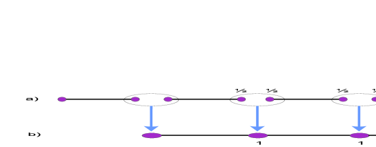
Figure 1: Color Online. A fully dimerized valence bond state, and the AKLT construction of a partially dimerized spin-1 state. The states in each bulb are projected to the symmetrized triplet. The parent Hamiltonian of the upper chain (a) has an interaction range of 3 lattice sites, while that of the lower chain (b) has a range of 2 sites.

Projection can also be used for other types of dimerized state as shown in figure (2-b) to construct states with arbitrary integer or half integer spins. For example in figure (2-b), looking at the number of valence bonds which are singlets and are not counted in the addition of spins in the virtual sites, one finds that the local Hamiltonians can be chosen as $h_{1}=\lambda_{3}P_{3}$ and $h_{2}=\lambda_{3}P_{3}+\lambda_{2}P_{2}$, where $P_{j}$ is the projector on spin-$j$ states and $\lambda_{j}$’s are positive coefficients. To assure translation invariance for the parent Hamiltonian one then takes $H=\sum_{j}h_{j,j+1}$ where $h=P_{3}$, is the operator common to both $h_{1}$ and $h_{2}$. Needless to say, this construction can be generalized by taking different alternating number of dimers in the virtual chain. This is also the basic idea behind the exactly solvable spin-3/2 spin systems on the honeycomb lattice [11] or more generally the basic idea behind PEPS, or Projected Entangled Pair States [12], which has only recently been discussed in the literature.

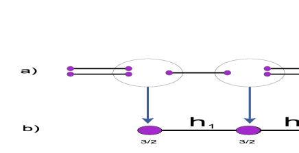
Figure 2: Color Online. An example of a dimerized state with alternating spin pattern and the AKLT construction of spin 3/2 chain. The interaction ranges are similar to that of figure (1) .

In the course of time, the basic idea of AKLT, which in turn was inspired by the work of Majumdar and Ghosh [6], led to the development of finitely correlated or matrix product representation of states [13, 14, 15], a representation which when existing, greatly facilitates the calculation of many properties of the ground states of quantum systems [8, 15, 16, 17, 18, 19, 20, 21, 22, 23, 24, 25, 26].
The Matrix Product (MP) representation was also found to be closely related with the success of density matrix renormalization group [27, 28, 29].

When considering spin chains, the basic continuous symmetry is the rotation symmetry captured by the $su(2)$ group, and there has been many different and equivalent implementations of this symmetry in matrix product states [21, 22, 25, 26, 29]. While a lot of progress has been made in defining matrix product states, having specific symmetries, to our knowledge the original AKLT variety of states, have not been cast into a simple and uniform matrix product form for both integer and non-integer spins. For the integer case however, such a formulation has been reported in [30]. There is no doubt that such a representation, will be of utmost importance for further study of AKLT models, and even for similar models on more general geometries like the Bethe Lattice [31].

To ensure invariance of the Matrix Product State (MPS) under rotation, it is sufficient that the elementary matrices used in the definition of the MPS constitute a representation of spherical tensor operators of a specific rank. The rank of the tensor depends on the spin of the actual lattice and the dimension of the representation determines the dimension of the auxiliary matrices. Finding a simple and minimal-dimensional representation for such tensors, constitute the basic problem in constructing rotationally invariant MPS, both for spin chain, spin ladders, or two dimensional lattices.

What we will do in this paper is to provide a uniform and simple matrix product representation for all the AKLT, or valence bond states and even more general states. The starting point of our analysis is a simple and compact representation of spherical tensor operators of any rank, integer or half integer. These tensors enable us to define MP representations for Majumdar-Ghosh states, (which are the ancestors of AKLT states) and their generalization to arbitrary spins, and then we will use them to construct MP representation for partially dimerized states. We then use projection method to find MP representations for arbitrary spin chains, with nearest neighbor interaction. The parallel with the AKLT construction is simple: the basic idea is to replace a collection of $2s$ spin-1/2 dimers or valence bonds with a single spin-$s$ valence bond and represent the states constructed from these spin-$s$ valence bonds as MPS.

Besides having the benefit of calculability, when we have an MPS representation, the very method of MPS allows us to find a larger family of Hamiltonians than the AKLT method. This larger family, with its larger number of couplings will enable us to better adjust or approximate an exactly solvable Hamiltonian with realistic situations. We will see an example of this in this paper.

The structure of this paper is as follows: In section 2 we review the matrix product formalism [13, 14, 15] in a language which we find convenient [21] for further developments. In particular we emphasize the symmetry properties of the ground state and the Hamiltonian. In section 3 we will introduce a compact formula for spherical tensors of rank $s$ (integer or half integer) and use it to construct dimerized states of arbitrary integer or half-integer spins in section (4). These are the generalization of Majumdar-Ghosh states, or fully dimerized states, to arbitrary spins. We then go on in section (5) to define MP representations for other types of dimerized states. In section (6) we find MP representations for AKLT/VBS states. The core of this section is the definition of new kinds of tensors, which play the role of auxiliary matrices for the MP representations of these states. Section (7) is devoted to some specific examples, where more detailed properties of some of the states and their parent Hamiltonians are derived. We conclude the paper with a discussion.

2 Matrix Product States

Let us first make a quick review of the matrix product states in a language which we find convenient [21, 22]. For more detailed reviews of the subject, the reader can consult a more comprehensive review article like [23] or any of the many works where specific examples have been studied [8, 21, 22, 16, 17, 18, 20, 19, 24, 25, 26].

Consider a ring of $N$ sites, where each site describes a $d-$level state. The Hilbert space $C^{d}$ of each site is spanned by the basis vectors $|i\rangle,\ \ i=0,\cdots,d-1$. A state

$$|\Psi\rangle=\sum_{i_{1},i_{2},\cdots,i_{N}}\Psi_{i_{1}i_{2}\cdots i_{N}}|i_{1}i_{2}\cdots i_{N}\rangle$$ (3)

is called a matrix product state if there exist $D$ dimensional matrices $A_{i}\in C^{D\times D},\ \ i=0,\cdots,d-1$, such that

$$\Psi_{i_{1}i_{2}\cdots i_{N}}=\frac{1}{\sqrt{Z}}tr(A_{i_{1}}A_{i_{2}}\cdots A_{i_{N}}),$$ (4)

where $Z$ is a normalization constant. This constant is given by $Z=tr(E^{N}),$ where $E=\sum_{i=0}^{d-1}A_{i}^{*}\otimes A_{i}$. Note that we are here considering homogeneous matrix product states where the matrices depend on the value of the spin at each site and not on the site itself. More general MPS’s can be defined where the matrices depend also on the position of the sites [23].

The collection of matrices $\{A_{i}\}$ and $\{\mu UA_{i}U^{-1}\}$, where $\mu$ is an arbitrary complex number, both lead to the same matrix product state, the freedom in scaling with $\mu$, is due to its cancelation with $Z$ in the denominator of (4). This freedom will be useful when we discuss symmetries. There has been discussions on the symmetry of matrix product states in the literature [13, 14, 19, 21, 25, 26], here we use the language or notation used in [21].

2.1 Symmetries of the ground state

Consider a local continuous symmetry operator $R$ acting on a site as $R|i\rangle=R_{ji}|j\rangle$ where summation convention is being used. $R$ is a $d$ dimensional unitary representation of the symmetry. A global symmetry operator ${\cal R}:=R^{\otimes N}$ will then change this state to another matrix product state

$$\Psi_{i_{1}i_{2}\cdots i_{N}}\longrightarrow\Psi^{\prime}_{i_{1}i_{2}\cdots i_{N}}:=tr(A^{\prime}_{i_{1}}A^{\prime}_{i_{2}}\cdots A^{\prime}_{i_{N}}),$$ (5)

where

$$A^{\prime}_{i}:=R_{ij}A_{j}.$$ (6)

The state $|\Psi\rangle$ is invariant (i.e. a singlet) under this symmetry if there exist an operator $U(R)$ such that

$$R_{ij}A_{j}=U^{-1}(R)A_{i}U(R).$$ (7)

Repeating this transformation and using the group multiplication of the transformations $R$, puts the constraint

$$U_{R^{\prime}}U_{R}=U_{R^{\prime}R}.$$ (8)

Thus $U(R)$ is a $D$ dimensional representation of the symmetry $R$. In case that $R$ is a continuous symmetry with generators $T_{a}$, equation (7), leads to

$$(T_{a})_{ij}A_{j}=[{\cal T}_{a},A_{i}],$$ (9)

where $T_{a}$ and ${\cal T}_{a}$ are the $d-$ and $D-$dimensional representations of the Lie algebra of the symmetry.

2.2 Symmetries of the Hamiltonian:

Given a matrix product state, the reduced density matrix of $k-$ sites is given by

$$\rho_{i_{1}\cdots i_{k},j_{1}\cdots j_{k}}=\frac{tr((A_{i_{1}}^{*}\cdots A_{i_{k}}^{*}\otimes A_{j_{1}}\cdots A_{j_{k}})E^{N-k})}{tr(E^{N})}.$$ (10)

The null-space of this reduced density matrix contains the subspace spanned by the solutions of

$$\sum_{j_{1},\cdots,j_{k}=0}^{d-1}c_{j_{1}\cdots j_{k}}A_{j_{1}}\cdots A_{j_{k}}=0.$$ (11)

Let the null space of the reduced density matrix of $k$ adjacent sites, denoted by $\Delta_{k}$, be spanned by the orthogonal vectors $|e_{\alpha}\rangle,\ \ \ (\alpha=1,\cdots,s\geq d^{k}-D^{2})$. Then we can construct the local hamiltonian acting on $k$ consecutive sites as

$$h:=\sum_{\alpha=1}^{s}\lambda_{\alpha}|e_{\alpha}\rangle\langle e_{\alpha}|,$$ (12)

where $\lambda_{\alpha}$’s are positive constants. These constants together with the parameters of the vectors $|e_{\alpha}\rangle$ inherited from those of the original matrices $A_{i}$, determine the total number of coupling constants of the Hamiltonian. If we call the embedding of this local Hamiltonian into the sites $l$ to $l+k$ by $h_{l,l+k}$ then the full Hamiltonian on the chain is written as

$$H=\sum_{l=1}^{N}h_{l,l+k}.$$ (13)

The state $|\Psi\rangle$ is then a ground state of this hamiltonian with vanishing energy. See [21] for a more detailed discussion of the above points.

A Hamiltonian derived as above does not have any particular symmetry. Indeed the above class include all types of Hamiltonians which have the matrix product state as their ground state. A subclass of these Hamiltonians however do have the symmetry of the ground state. Consider equation (11), multiplying both sides of this equation by $U^{-1}(R)$ from left and $U(R)$ from right, and using (7), we find that if $c_{i\cdots j}$ is a solution of (11), then $R_{i,i^{\prime}}\cdots R_{j,j^{\prime}}c_{i^{\prime},\cdots j^{\prime}}$ is also a solution of the same equation, that is:

$$R_{i,i^{\prime}}\cdots R_{j,j^{\prime}}c_{i^{\prime},\cdots j^{\prime}}=\lambda(R)c_{i,\cdots j}.$$ (14)

This means that the null space of the reduced density matrix is an invariant subspace under the action of the symmetry group $R^{\otimes k}$. Thus the null vectors $|e_{\alpha}\rangle$ transform into each other under the action of the reducible representation $R^{\otimes k}$. Such vectors can be classified into multiplets such that each multiplet transforms under one irreducible representation of the group $R$. Let the states transforming under the irreducible representation $D^{\mu}$ of the group, be denoted by $|e^{\mu}_{\beta}\rangle$. Then the operators $h^{\mu}=\sum_{\beta}|e^{\mu}_{\beta}\rangle\langle e^{\mu}_{\beta}|$, is a scalar under the action of the group, that is

$$[D^{\mu},h^{\mu}]=0.$$ (15)

Hence to ensure the symmetry of the local Hamiltonian we write it as

$$h_{i,i+k}=\sum_{\mu}{\lambda_{\mu}}h^{\mu}=\sum_{\mu,\beta}\lambda_{\mu}|e^{\mu}_{\beta}\rangle\langle e^{\mu}_{\beta}|,$$ (16)

where the number of free couplings $\lambda_{\mu}$ is equal to the number of multiplets which span the null space $\Delta_{k}$.

3 A new representation for spherical tensors of arbitrary rank

We are now equipped with generalities about matrix product states and their symmetry properties. In this section we specialize the above discussion to construction of spin-s MPS invariant under rotation in spin space. For such a chain we take local Hilbert space to be spanned by the $d=2s+1$ states of a spin-$s$ particle, i.e. the states $\{|s,m\rangle,m=-s,\cdots s\}$. Let us denote the $D$ dimensional matrix assigned to the local configuration $m$ by $A_{s,m}$. Rotational symmetry in the spin space now demands that the matrices $A_{s,m}$ form an irreducible tensor operator of rank $s$ in the space of $D$ dimensional square matrices. In view of (9), we should find $2s+1$ matrices $A_{s,m}$ such that the following relations are satisfied

$$[L_{z},A_{s,m}] = mA_{s,m}$$ (17)

$$[L_{+},A_{s,m}] = \sqrt{s(s+1)-m(m+1)}A_{s,m+1}$$ (18)

$$[L_{-},A_{s,m}] = \sqrt{s(s+1)-m(m-1)}A_{s,m-1}$$ (19)

where $L_{z}$, $L_{+}$ and $L_{-}$ are the $D$ dimensional representations (not necessarily irreducible) of the Lie algebra of $su(2)$:

$$[L_{z},L_{\pm}]=\pm L_{\pm}\hskip 28.45274pt[L_{+},L_{-}]=2L_{z}.$$ (20)

Remark: For simplicity, we will use the notation $|m\rangle$ and $A_{m}$ instead of $|s,m\rangle$ and $A_{s,m}$ respectively, when the label $s$ is clear from the context.

It is crucial to note that it is not always possible to find tensor operators of a given rank for a given $D$ dimensional representation. For example while there is tensor of rank one, in two dimensions, given by

$$A_{1}=-\sqrt{2}\sigma_{+},\ \ \ \ A_{0}=\sigma_{z},\ \ \ \ A_{-1}=\sqrt{2}\sigma_{-},$$ (21)

leading to the spin-1 AKLT model [5], with parent Hamiltonian (2), there is no rank $1/2$ tensor operator in $2$ dimensions. By this we mean that if we take $D=2$, then there is no non-zero solution for the following system of matrix equations

$$[L_{z},A_{\pm}] = \pm\frac{1}{2}A_{\pm}$$ (22)

$$[L_{+},A_{+}] = 0,\ \ \ \ [L_{+},A_{-}]=A_{+},$$ (23)

$$[L_{-},A_{+}] = A_{-},\ \ \ \ [L_{-},A_{-}]=0.$$ (24)

Therefore the first task for construction of rotationally invariant matrix product states for quantum spin chains or quantum ladders is to have a compact expression for spherical tensors of arbitrary rank.

A possible procedure for obtaining spherical tensors of integer rank is to take two low-rank (possibly identical) tensors and decompose their ordinary or tensor product by the Clebsh-Gordon series to obtain irreducible tensors of higher rank. In fact if $A_{s,m}$ and $A_{s^{\prime},m^{\prime}}$ are two spherical tensors, then one can form the product $A_{s,m}A_{s^{\prime},m^{\prime}}$ (if their dimensions are the same) or $A_{s,m}\otimes A_{s^{\prime},m^{\prime}}$ (otherwise) and decompose the products by using the Clebsh-Gordon coefficients to obtain spherical tensors of higher rank. For example take the AKLT tensor of rank one. Ordinary multiplication of this tensor, does not give a tensor of rank 2, since $\sigma_{+}^{2}=0$, however its tensor multiplication gives a tensor of rank two of dimension 4, i.e. $A_{2,2}=2\sigma_{+}\otimes\sigma_{+}$, etc. In this way the product of two rank-1 tensors can be decomposed to give a rank-2, a rank-1 and rank-0 tensor. The obtained tensors can again be multiplied with other tensors and decomposed to obtain tensors of even higher rank. This procedure however has several drawbacks: first the dimensions of the matrices will grow very fast as we increase the rank of tensors, second it requires multiple use of Clebsh-Gordon coefficients which makes the final expression of the tensors, especially for high-rank tensors, quite cumbersome and not useful. Another useful procedure, is to invoke the Wigner-Eckart theorem which decomposes the matrix elements of any spherical tensor in the angular momentum basis, to an angular part, which is the Clebsh-Gordon coefficient and a reduced part, which essentially defines the tensor. However this procedure does not always lead to a compact notation for the tensor operators themselves and the multiplication of such tensors requires heavy use of Glebsh-Gordon coefficients. In this paper we introduce a compact and transparent formula for spherical tensors of rank $s$, for $s$ integer or half integer, and use it to construct matrix product states for spin chains. For rank-$s$ tensors the dimensions of the matrices are $2s+2$, thus the dimension grows linearly with rank.

To construct the spherical rank-$s$ tensor, let us take the orthonormal basis $\{|s,m\rangle,\ m=-s\cdots s\}$ of the spin $s$ representation and augment it by the single state $|\tilde{0}\rangle$, of the spin $0$ representation

$$\langle\tilde{0}|\tilde{0}\rangle=1,\ \ \ \ \langle\tilde{0}|s,m\rangle=\langle s,m|\tilde{0}\rangle=0.$$ (25)

On this larger space, the following is the reducible $s\oplus 0$ representation of angular momentum algebra:

$$L_{z}=\sum_{m=-s}^{s}m|s,m\rangle\langle s,m|$$ (26)

$$L_{+}=\sum_{m=-s}^{s}\sqrt{{s(s+1)-m(m+1)}}|s,m+1\rangle\langle s,m|$$ (27)

$$L_{-}=\sum_{m=-s}^{s}\sqrt{{s(s+1)-m(m-1)}}|s,m-1\rangle\langle s,m|.$$ (28)

Now it is readily verified that in this $2s+2$ dimensional space, the following matrices form an irreducible rank-$s$ spherical tensor, that is they satisfy the relations (17):

$$A_{s,m}:=|s,m\rangle\langle\ \tilde{0}|+(-1)^{s-m}|\tilde{0}\rangle\langle s,-m|$$ (29)

where $-s\leq m\leq s$.
It is important to note that the rank of these tensors can be integer or half integer. Such operators transform as an irreducible rank $s$ tensor in the space which carries the reducible representation $s\oplus 0$.

Note: One can define the tensors more generally as

$$A_{s,m}:=a|s,m\rangle\langle\ \tilde{0}|+b(-1)^{m}|\tilde{0}\rangle\langle s,-m|$$

where $a$ and $b$ are arbitrary numbers, however these tensors are equivalent to the previous ones in the sense that they reduce to them by a suitable unitary transformation. The factor $(-1)^{s}$ is inserted in the definition to ensure that no complex number enters the expression for half-integer ranks.

While there are many representations for spherical tensors of different ranks, and these have been used in different works to construct various examples of invariant MPS [16, 17, 18, 19, 21, 25, 26], to our knowledge the representation (29) is introduced for the first time. In the sequel we show that this representation is very general, in the sense that we can use it to find MP representations for all the variety of AKLT states, including the Majumdar-Ghosh or fully dimerized states of arbitrary spin, the partially dimerized states, and also the various states which are found from these partially dimerized states by different types of projection. Even more, one can construct other states not listed in the original AKLT papers, these are the symmetry breaking states.

4 The spin-s fully dimerized or Majumdar-Ghosh states

Using the definition of $A_{m}$ we find:

$$A_{m_{1}}A_{m_{2}}\cdots A_{m_{2N}} = \prod_{i=1}^{N}(-1)^{s-m_{2i-1}}\delta_{m_{2i-1},-m_{2i}}|\tilde{0}\rangle\langle\tilde{0}|$$ (30)

$$+ (-1)^{s-m_{2N}}\prod_{i=1}^{N-1}(-1)^{s-m_{2i}}\delta_{m_{2i},-m_{2i+1}}|m_{1}\rangle\langle-m_{2N}|$$ (31)

Taking the trace we find

$$Tr(A_{m_{1}}\cdots A_{m_{2N}})=\prod_{i=1}^{N}(-1)^{s-m_{2i-1}}\delta_{m_{2i-1},-m_{2i}} + \prod_{i=1}^{N}(-1)^{s-m_{2i}}\delta_{m_{2i},-m_{2i+1}}.$$ (32)

Inserting this into (3-4) the final simple form of the matrix product ground state is obtained as

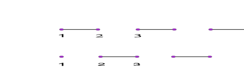
Figure 3: Color Online. The fully dimerized spin-s states in equation (33).

$$|\psi\rangle\equiv|\phi_{1}\rangle+|\phi_{2}\rangle=|S\rangle_{12}|S\rangle_{34}\cdots|S\rangle_{2N-1,2N}+|S\rangle_{23}|S\rangle_{45}\cdots|S\rangle_{2N,1},$$ (33)

where the singlet states $|S\rangle$ are given by

$$|S\rangle=\frac{1}{\sqrt{2s+1}}\sum_{m}(-1)^{s+m}|m,-m\rangle.$$ (34)

Note that $|S\rangle$ is a singlet state, i.e. $L_{z}|S\rangle=L_{+}|S\rangle=L_{-}|S\rangle=0$. Thus $|\phi_{1}\rangle$ is a juxtaposition of spin-s dimers on sites $(1,2),(3,4),\cdots(2N-1,2N)$ and $|\phi_{2}\rangle$ is a one-site translation of $|\phi_{1}\rangle,$ i.e. a collection of spin-s dimers on sites $(2,3),(4,5),\cdots(2N,1)$, figure (3).

5 Other types of dimerized states

A general dimerized state is one which is shown in figure (4-a), where each line stands for a spin-1/2 dimer. The numbers of dimers are $2s$ and $2s^{\prime}$ respectively. In our representation, we replace 2s spin-1/2 dimers with a single spin-s dimer, as in figure (4-b). Such a state has simple MPS representation, in the form

$$|\psi\rangle=\sum tr(A_{m_{1}}A_{m_{2}}B_{m^{\prime}_{1}}B_{m^{\prime}_{2}}A_{m_{3}}A_{m_{4}}B_{m^{\prime}_{3}}B_{m^{\prime}_{4}}\cdots)|m_{1}m_{2}m^{\prime}_{1}m^{\prime}_{2}m_{3}m_{4}m^{\prime}_{3}m^{\prime}_{4}\cdots\rangle\ ,$$ (35)

where the matrices $\{A_{m}\}$ and $\{B_{m^{\prime}}\}$ are embedding of the rank-$s$ and rank-$s\prime$ tensors (29) into a representation spanned by the vectors $\{|\tilde{0}\rangle,|s,m\rangle,|s^{\prime},m^{\prime}\rangle\}$, i.e. the direct sum representation $s\oplus s^{\prime}\oplus 0$. In fact it is readily found that with

$$A_{s,m}\equiv A_{m} = |s,m\rangle\langle\tilde{0}|+(-1)^{s-m}|\tilde{0}\rangle\langle s,-m|,$$ (36)

$$A_{s^{\prime},m^{\prime}}\equiv B_{m^{\prime}} = |s^{\prime},m^{\prime}\rangle\langle\tilde{0}|+(-1)^{s^{\prime}-m^{\prime}}|\tilde{0}\rangle\langle s^{\prime},-m^{\prime}|,$$ (37)

we have

$$A_{m_{1}}A_{m_{2}}B_{m^{\prime}_{1}}B_{m^{\prime}_{2}}=(-1)^{s-m_{1}}\delta_{m_{1},-m_{2}}(-1)^{s^{\prime}-m^{\prime}_{1}}\delta_{m^{\prime}_{1},-m^{\prime}_{2}}|\tilde{0}\rangle\langle\tilde{0}|$$ (38)

which readily yields the following partially dimerized form for the state (35):

$$|\psi\rangle=|S\rangle_{12}|S^{\prime}\rangle_{34}|S\rangle_{56}|S^{\prime}\rangle_{78}\cdots$$ (39)

where $|S\rangle$ and $|S^{\prime}\rangle$ are respectively spin-$s$ and spin-$s^{\prime}$ singlets defined in (34).

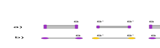
Figure 4: Color Online. 2$s$ valence bonds (spin 1/2 singlets) in the AKLT construction, are replaced in our work, with a single spin-s valence bond, which is MPS representable by the matrix (35).

One can construct even more general states, i.e. the symmetry breaking states of the form shown in figure (5) where the dimers are interspaced by spins which align in a particular direction. Consider the state

$$|\psi\rangle=tr(A_{{}_{m_{1}}}A_{{}_{m_{2}}}C_{{}_{m_{3}}}A_{{}_{m_{4}}}A_{{}_{m_{5}}}C_{{}_{m_{6}}}\cdots)|m_{1},m_{2},m_{3},m_{4},m_{5},m_{6},\cdots\rangle$$ (40)

where $A_{m}$ is of the form (29) and $C_{m}=\alpha_{m}|\tilde{0}\rangle\langle\tilde{0}|$, in which $\alpha_{m}$’s ($-s\leq m\leq s$) are arbitrary complex numbers. Then the MPS represents a symmetry breaking state shown in figure (5), where spins, $3,6,\cdots$ are aligned in the state $|\alpha\rangle:=\sum_{m=-s}^{s}\alpha_{m}|s,m\rangle$ and the rest of the sites are dimerized. A suitable projection of these states, gives symmetry-breaking non-dimerized states [32].

Figure 5: Color Online. The tensors (29) can also be used to construct symmetry-breaking matrix product states. .

6 The AKLT/VBS states

In the AKLT models, one can use the fully dimerized states and project them to states which are called VBS states. While the parent Hamiltonian of the fully dimerized states has an interaction range of 3 sites, the VBS states which are obtained by projection have parent Hamiltonians with interaction range of 2 sites. The method is explained in figure (6), where we use a single spin-s dimer to replace 2s spin-1/2 dimers in the original method of AKLT.

The lower state is obtained by projecting the states inside each bulb in the upper chain onto the symmetrized spin sector with total spin $s+s^{\prime}$. It is now obvious how the parent Hamiltonian of the lower chain, the Hamiltonian which has this state as its ground state, should be constructed. Consider the first bond in figure (6) whose local Hamiltonian is denoted by $h_{1}$. Due to the $2s^{\prime}$ singlets, between the two bulbs, here we are only summing over two spin $s$ states, instead of the apparent two spin $s$ and two spin-$s^{\prime}$ states. Hence all the projectors $P_{j}$, with $2s+1\leq j\leq 2s+2s^{\prime}$, annihilate this bond, i.e. the local Hamiltonian $h_{1}$, can be constructed as a linear superposition of all the above projectors with positive coefficients. By the same reasoning the local Hamiltonian $h_{2}$ can be a linear superposition of all projectors $P_{k}$, with $2s^{\prime}+1\leq k\leq 2s+2s^{\prime}$. Thus to construct a translation-invariant Hamiltonian, the parent Hamiltonian of the lower state can be constructed as

$$H=\sum_{i}h_{i,i+1},$$ (41)

where

$$h=\sum_{j=max(2s,2s^{\prime})+1}^{2s+2s^{\prime}}\lambda_{j}P_{j},$$ (42)

where $P_{j}$’s are the projectors on spin $j$ sector of two sites and $\lambda_{j}$ are positive coefficients.

Note that the state on the lower chain is no longer dimerized, i.e. spins which are further apart than one lattice spacing, are correlated. Needless to say, the projection method, although elegant in principle, is not suitable for calculation of many properties of the state. Having a matrix product representation for this state, turns all calculations into a straightforward and handy procedure. In this section we show that the irreducible tensors introduced in section (3), provides a MP representation for these states in a very simple way.

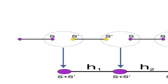
Figure 6: Color Online. The projection method: From a partially or fully dimerized state, whose parent Hamiltonian has interaction range 3, an AKLT/VBS state is constructed whose parent Hamiltonian has interaction range 2. The form of the Hamiltonian is given in equations (41) and (42).

The starting point of our procedure is however not to use $2s$ and $2s^{\prime}$ spin-1/2 dimers as in figure (4-a), rather we use equivalently one spin-s and one spin-s’ singlets as in figure (4-b), for which we have already a MP representation. The spin-s and spin-s’ dimers come from rank-s and rank-s’ tensors (29). We multiply and symmetrize these two tensors to obtain a new tensor whose highest component is given by

$$V_{s+s^{\prime},s+s^{\prime}}=A_{s,s}A_{s^{\prime},s^{\prime}}+A_{s^{\prime},s^{\prime}}A_{s,s}.$$ (43)

From the explicit form of the tensors in (29), one sees that,

$$V_{s+s^{\prime},s+s^{\prime}}:=|s,s\rangle\langle s^{\prime},-s^{\prime}|+|s^{\prime},s^{\prime}\rangle\langle s,-s|.$$ (44)

Note that this tensor lives in the $2s+2s^{\prime}+2$ dimensional space spanned by independent vectors $\{|s,m\rangle,\ |s^{\prime},m^{\prime}\rangle,\ -s\leq m\leq s,\ -s^{\prime}\leq m^{\prime}\leq s^{\prime}\}$.

It is readily verified that

$$[L_{z},V_{s+s^{\prime},s+s^{\prime}}] = (s+s^{\prime})V_{s+s^{\prime},s+s^{\prime}}$$ (45)

$$[L_{+},V_{s+s^{\prime},s+s^{\prime}}] = 0.$$ (46)

Therefore $V_{s+s^{\prime},s+s^{\prime}}$ is indeed the highest-weight component of a spherical tensor of rank $s+s^{\prime}$. Other components are obtained by successive commutations with $L_{-}$. For example, we have

$$V_{s+s^{\prime},s+s^{\prime}-1} := \sqrt{\frac{s}{s+s^{\prime}}}(|s,s-1\rangle\langle s^{\prime},-s^{\prime}|-|s^{\prime},s^{\prime}\rangle\langle s,-s+1|)$$ (47)

$$+ \sqrt{\frac{s^{\prime}}{s+s^{\prime}}}(|s^{\prime},s^{\prime}-1\rangle\langle s,-s|-|s,s\rangle\langle s^{\prime},-s^{\prime}+1|).$$ (48)

The new spherical tensors have the interesting property that they lead to a non-empty null space $\Delta_{2}$. In fact it can be verified that these tensors have a peculiar fusion rule (decomposition of the product into irreducible representations), which exactly matches the fusion rule of the original $2s$ and $2s^{\prime}$ valence bonds in a symmetric way. In the present formalism, this symmetry causes the final local Hamiltonian $h$ to contain projectors common to both $h_{1}$ and $h_{2}$ (figure (6)) in the AKLT construction. Using the notation $V_{s}$ to denote the whole multiplet $V_{s,m},\ -s\leq m\leq s$, the fusion rule of our tensors is

$$V_{s+s^{\prime}}\otimes V_{s+s^{\prime}}=\bigoplus_{j=0}^{max(2s,2s^{\prime})}c_{j}V_{j}.$$ (49)

Thus the multiplets $V_{j}$ with $max(2s,2s^{\prime})+1\leq j\leq 2(s+s^{\prime})$ are absent, i.e. identically vanish, in the decomposition of the left hand side tensors. In the language of matrix product formalism, section (2), this means that the null-space of the two-site density matrix, contains the multiplet of states which transform as spin $j$ representations with $max(2s,2s^{\prime})+1\leq j\leq 2(s+s^{\prime})$. Therefore the local Hamiltonian annihilating the dimerized state, can be constructed from the projectors to these multiplets, namely

$$h=\sum_{j=max(2s,2s^{\prime})+1}^{2s+2s^{\prime}}\lambda_{j}P_{j},$$ (50)

where $P_{j}$’s are projectors on spin $j$ and $\lambda_{j}$ are positive coefficients. It requires tedious and lengthy calculations which may not be illuminating to prove (49) in general. Instead we will give an idea of the proof by way of examples. First of all, it is readily seen from (44) that $s,s^{\prime}\neq 0,$

$$V_{s+s^{\prime},s+s^{\prime}}^{2}=0,$$

but this is the top state of the multiplet $V_{2s+2s^{\prime}}$ and hence this multiplet is absent in the right hand side of (49). In the same way one can also show from (44) and (47) that the top state of the multiplet $V_{2s+2s^{\prime}-1}$ is zero. This pattern repeats until we arrive at the multiplet $V_{max(2s,2s^{\prime})}$. We will give a more detailed and concrete example in section (7).

7 Examples

Up until now we have been able to use our spherical tensors (29), in a uniform manner to construct all the variety of valence-bond states in the AKLT constrution. In this section, we will provide a few concrete examples.

7.1 Properties of fully dimerized or spin-s Majumdar-Ghosh states

First we calculate the normalization of fully dimerized states $|\Psi^{\pm}\rangle.$ The basic tool which we use is the following easily verified equation between the singlets, where $1,2,3$ and $4$ are any four different and not necessarily adjacent sites:

$$_{{}_{23}}\langle S|S\rangle_{{}_{12}}|S\rangle_{{}_{34}}=\frac{\epsilon}{2s+1}|S\rangle_{{}_{14}},$$ (51)

where

$$\epsilon=\left\{\begin{array}[]{ll}1&s={\rm integer}\\ \\ -1&s={\rm half\ integer}\end{array}\right.$$

This relation which we will use repeatedly in the following is depicted graphically in figure (7). Here a bulb around two sites $2,3$ means that it has been multiplied from the left by a singlet ${}_{{}_{2,3}}\langle S|$. Repeatedly using equation (51) or the graph (7), as in figure (8), will give

$$\langle\phi_{1}|\phi_{2}\rangle=\frac{\epsilon^{N}}{(2s+1)^{N-1}}$$ (52)

from which we obtain the normalization

$$\langle\Psi^{\pm}|\Psi^{\pm}\rangle=2(1\pm\frac{\epsilon^{N}}{(2s+1)^{N-1}}).$$ (53)

In order to find the correlations we use the following equations,

$${}_{{}_{12}}\langle S|{\bf s}_{1}\cdot{\bf s}_{2}|S\rangle_{{}_{12}}=-s(s+1),$$ (54)

and

$${}_{{}_{23}}\langle S|{\bf s}_{1}\cdot{\bf s}_{2}|S\rangle_{{}_{12}}|S\rangle_{34}=-s(s+1)\ _{{}_{23}}\langle S|S\rangle_{{}_{12}}|S\rangle_{{}_{34}}=-\frac{s(s+1)\epsilon^{N}}{2s+1}|S\rangle_{{}_{14}},$$ (55)

which readily gives

$$\langle\phi_{1}|{\bf s}_{1}\cdot{\bf s}_{2}|\phi_{1}\rangle=-s(s+1),\hskip 28.45274pt\langle\phi_{2}|{\bf s}_{1}\cdot{\bf s}_{2}|\phi_{2}\rangle=0.$$ (56)

Again the cross-product terms is calculated with the help of graph (8),

$$\langle\phi_{1}|{\bf s}_{1}\cdot{\bf s}_{2}|\phi_{2}\rangle=-s(s+1)\langle\phi_{1}|\phi_{2}\rangle=-s(s+1)\frac{\epsilon^{N}}{(2s+1)^{N-1}}.$$ (57)

Putting these together we find the final form of the correlation functions:

$$\frac{\langle\Psi^{\pm}|{\bf s}_{1}\cdot{\bf s}_{2}|\Psi^{\pm}\rangle}{\langle\Psi^{\pm}|\Psi^{\pm}\rangle}=-\frac{s(s+1)}{2}\frac{(2s+1)^{N-1}\pm 2\epsilon^{N}}{(2s+1)^{N-1}\pm\epsilon^{N}}.$$ (58)

Figure 7: Color Online. The graphical representation of equation (51). A bulb around 2 and 3, means that the state has been multiplied from the left by ${}_{2,3}\langle S|$, leaving the singlet on the right hand side. Note that the labels 1, 2, 3 and 4, denote any four sites.

Figure 8: Color Online. The repeated use of the graph (7) for calculating the cross product terms $\langle\phi_{1}|\phi_{2}\rangle$.

To construct the parent Hamiltonian of such states, we use (11) and find the null-space of the reduced density matrices of three consecutive sites $\Delta_{3}$, (two consecutive sites have no non-trivial null space in this model). From (29) we have

$$A_{m}A_{m^{\prime}}A_{m^{\prime\prime}}=(-1)^{s-m^{\prime}}\delta_{m^{\prime},-m^{\prime\prime}}|m\rangle\langle\tilde{0}|+\delta_{m^{\prime},-m}(-1)^{2s-m-m^{\prime\prime}}|\tilde{0}\rangle\langle-m^{\prime\prime}|.$$ (59)

To find the null space $\Delta_{3},$ we need to solve the matrix equation

$$\sum_{m,m^{\prime},m^{\prime\prime}}c_{m,m^{\prime},m^{\prime\prime}}A_{m}A_{m^{\prime}}A_{m^{\prime\prime}}=0,$$ (60)

which yields the following conditions:

$$\sum_{m}(-1)^{m}C_{m^{\prime},m,-m} = 0\hskip 28.45274pt\forall m^{\prime}$$ (61)

$$\sum_{m}(-1)^{m}C_{m,-m,m^{\prime}} = 0\hskip 28.45274pt\forall m^{\prime}.$$ (62)

These conditions can be re-expressed in a more useful form, namely the null space $\Delta_{3}$ is spanned by vectors of the form

$$|\chi\rangle=\sum_{m,m^{\prime},m^{\prime\prime}}c_{m,m^{\prime},m^{\prime\prime}}|m,m^{\prime},m^{\prime\prime}\rangle$$ (63)

which are perpendicular to the state (34) i.e.

$$_{12}\langle S|\chi\rangle=0,\ \ \ \ \ \ _{23}\langle S|\chi\rangle=0,$$ (64)

where the subscripts indicate the embedding of $\langle S|$ into the local spaces of three consecutive spins. Note that the factor $\sqrt{2s+1}$ has been inserted so that the state $|S\rangle$ be normalized. We will later use these equations to clarify the form of the Hamiltonian, but first let us derive an explicit form for the ground state.

One is tempted to ask if $|\phi_{1}\rangle$ or $|\phi_{2}\rangle$ are ground states separately. The answer is positive. To see this, note that the Hamiltonian is written in the form

$$H=\sum_{k=1}^{2N}h_{k,k+1,k+2},$$ (65)

where $h$ is the sum of projectors on the null space $\Delta_{3}$, i.e.

$$h=\sum_{\alpha}\lambda_{\alpha}|e_{\alpha}\rangle\langle e_{\alpha}|,\hskip 28.45274pt|e_{\alpha}\rangle\in\Delta_{3}.$$ (66)

Here $\{|e_{\alpha}\rangle\}$ is a basis for $\Delta_{3}$ and from (64) we know that $\langle e_{\alpha}|S\rangle_{12}=\langle e_{\alpha}|S\rangle_{23}\ \ \ \ \forall\ \ \alpha$. This implies that $H|\phi_{1}\rangle=H|\phi_{2}\rangle=0$. Each of the dimerized states $|\phi_{1}\rangle$ and $|\phi_{2}\rangle$, break the translational symmetry of the Hamiltonian. Finally let us also derive the parent Hamiltonians for the simplest cases, namely spin 1/2 which is well-known and spin-1 Majumdar-Ghosh states.

a: The parent Hamiltonian for Spin-1/2 dimerized state

Using the standard notation $|+\rangle:=|\frac{1}{2},\frac{1}{2}\rangle,\ \ |-\rangle:=|\frac{1}{2},\frac{-1}{2}\rangle$ we order the states of auxiliary space, as $\{|+\rangle,|\tilde{0}\rangle,|-\rangle\}$. Then from (29) we have

$$A_{+} = |+\rangle\langle\tilde{0}|+|\tilde{0}\rangle\langle-|=\left(\begin{array}[]{ccc}0&1&0\\ 0&0&1\\ 0&0&0\end{array}\right)$$ (70)

$$A_{-} = |-\rangle\langle\tilde{0}|-|\tilde{0}\rangle\langle+|=\left(\begin{array}[]{ccc}0&0&0\\ -1&0&0\\ 0&1&0\end{array}\right),$$ (74)

which transforms as a rank $1/2$ tensor with the generators given by

$$L_{z}=\left(\begin{array}[]{ccc}\frac{1}{2}&0&0\\ 0&0&0\\ 0&0&\frac{-1}{2}\end{array}\right),\ \ \ \ L_{+}=\left(\begin{array}[]{ccc}0&0&1\\ 0&0&0\\ 0&0&0\end{array}\right),\ \ \ \ \ L_{-}=\left(\begin{array}[]{ccc}0&0&0\\ 0&0&0\\ 1&0&0\end{array}\right).$$ (75)

The singlet states are $|S\rangle=\frac{1}{\sqrt{2}}(|+,-\rangle-|-,+\rangle)$. To find the parent Hamiltonian, we should solve equation (61), or what is the same thing, find states $|\chi\rangle\in C^{2}\otimes C^{2}\otimes C^{2}$ such that ${}_{12}\langle S|\chi\rangle=_{23}\langle S|\chi\rangle=0$. It is readily found that there are four such states:

$$|e_{1}\rangle = |+,+,+\rangle,$$ (76)

$$|e_{2}\rangle = \frac{1}{\sqrt{3}}(|+,+,-\rangle+|+,-,+\rangle+|-,+,+\rangle),$$ (77)

$$|e_{3}\rangle = \frac{1}{\sqrt{3}}(|-,-,+\rangle+|-,+,-\rangle+|+,-,-\rangle),$$ (78)

$$|e_{4}\rangle = |-,-,-\rangle.$$ (79)

The vectors $|e_{i}\rangle$ form the spin $\frac{3}{2}$ multiplet, and if they come with the same coefficients in $h$ in (66), the resulting Hamiltonian will be a scalar. It is known [22, 23] that in this case the parent Hamiltonian will be the Majumdar-Ghosh Hamiltonian, namely

$$H=\sum_{i}2\sigma_{i}\cdot\sigma_{i+1}+\sigma_{i}\cdot\sigma_{i+2}.$$

b: The parent Hamiltonian for Spin-1 fully dimerized state

Using the abbreviated notation $|1\rangle:=|1,1\rangle,\ |0\rangle:=|1,0\rangle,\ |\overline{1}\rangle:=|1,-1\rangle$, we have as the singlet state in $|S\rangle\in C^{3}\otimes C^{3}$,

$$|S\rangle=\frac{1}{\sqrt{3}}(|1,\overline{1}\rangle-|0,0\rangle+|\overline{1},1\rangle).$$ (80)

In order to find the null space $\Delta_{3}$, we note that due to $su(2)$ symmetry, equation (14), the basis vectors of $\Delta_{3}$ can be grouped into multiplets which transform irreducibly under $su(2)$. These multiplets come from the decomposition of $1\otimes 1\otimes 1$ representation, which decomposes as

$$1\otimes 1\otimes 1=3\oplus 2\oplus 2^{\prime}\oplus 1\oplus 1^{\prime}\oplus 1^{\prime\prime}\oplus 0.$$ (81)

However not all the above multiplets belong to $\Delta_{3}$. In order to determine those which are, we should check the conditions (61). It is sufficient to check these conditions only for the top state of each multiplet, since symmetry guarantees that the other states are present in $\Delta_{3}$, once the top state is present. With this insight we readily find the multiplets with the following top states are present in $\Delta_{3}$:

$$|e_{1}\rangle := |t_{3}\rangle=|1,1,1\rangle$$ (82)

$$|e_{2}\rangle := |t_{2}\rangle=|1,1,0\rangle-|0,1,1\rangle$$ (83)

$$|e_{3}\rangle := |t_{2^{\prime}}\rangle=|1,1,0\rangle-2|1,0,1\rangle+|0,1,1\rangle$$ (84)

$$|e_{4}\rangle := |t_{1}\rangle=|1,0,0\rangle+|0,0,1\rangle+3|\overline{1},1,1\rangle+3|1,1,\overline{1}\rangle-2|1,\overline{1},1\rangle-4|0,1,0\rangle$$ (85)

$$|e_{5}\rangle := |t_{0}\rangle=|1,\overline{1},0\rangle-|\overline{1},1,0\rangle-|1,0,\overline{1}\rangle+|\overline{1},0,1\rangle+|0,1,\overline{1}\rangle-|0,\overline{1},1\rangle,$$ (86)

where $|t_{j}\rangle$ denotes the top state of the spin-$j$ representation. One can verify that these are actually the top states by checking the equations $L_{z}|t_{j}\rangle=j|t_{j}\rangle,$ and $\ \ L_{+}|t_{j}\rangle=0$ and also that they really belong to $\Delta_{3}$ by checking ${}_{12}\langle S|e_{i}\rangle=_{23}\langle S|e_{i}\rangle=0$.

Having 5 different multiplets in the null space, means that the Hamiltonian has 5 different couplings which can be tuned. Of course one of the couplings can be set to unity by a choice of energy scale. Let’s call the projectors on the representation space $j$ by $P_{j}$. Then the local Hamiltonian $h$ will be

$$h=\lambda_{0}P_{0}+\lambda_{1}P_{1}+\lambda_{2}P_{2}+\lambda^{\prime}_{2}P_{2^{\prime}}+\lambda_{3}P_{3}.$$ (87)

Remark: It is important to note that the MPS formalism, gives a larger family of parent Hamiltonian than the original AKLT construction. In fact in the AKLT construction, the presence of projectors $P_{3}$, $P_{2}$ and $P_{2^{\prime}}$ and $P_{0}$ is automatic. However the presence of the new projector $P_{1}$ is the result of the MPS formalism.

The next step, which is not trivial, is to write the projectors in terms of local spin operators. The point is that on the decomposition (81) only some of the representations on the right hand side belong to $\Delta_{3}$. For those representations which occur with multiplicity one, we can easily find the expression of the corresponding projectors in terms of local spin operators. Let us denote the sum of spin operators on three sites by ${\bf S}$, i.e

$${\bf S}:={\bf S}_{1}+{\bf S}_{2}+{\bf S}_{3}.$$

The basis states of the representations on the right hand side of (81) are such that they block-diagonalize the generators and hence the operator ${\bf S}\cdot{\bf S}$. Let us denote the projectors on the totality of spin $j$ representations by ${\cal P}_{j}$, i.e. ${\cal P}_{0}=P_{0},\ \ {\cal P}_{1}:=P_{1}+P_{1^{\prime}}+P_{1^{\prime\prime}},\ \ \ {\cal P}_{2}=P_{2}+P_{2^{\prime}}$, and ${\cal P}_{3}=P_{3}$. Then we have the following system of equations $({\bf S}\cdot{\bf S})^{k}=\sum_{l=0}^{3}(l(l+1))^{k}{\cal P}_{l},\ k=0,1,2,3$, or more explicitly,

$$I = {\cal P}_{3}+{\cal P}_{2}+{\cal P}_{1}+{\cal P}_{0}$$ (88)

$${\bf S}\cdot{\bf S} = 12{\cal P}_{3}+6{\cal P}_{2}+2{\cal P}_{1}$$ (89)

$$({\bf S}\cdot{\bf S})^{2} = 144{\cal P}_{3}+36{\cal P}_{2}+4{\cal P}_{1}$$ (90)

$$({\bf S}\cdot{\bf S})^{3} = 343{\cal P}_{3}+125{\cal P}_{2}+27{\cal P}_{1}.$$ (91)

Inverting the above equations we find

$$720{\cal P}_{3} = 12{\bf S}\cdot{\bf S}-8({\bf S}\cdot{\bf S})^{2}+({\bf S}\cdot{\bf S})^{3}$$ (92)

$$144{\cal P}_{2} = -24{\bf S}\cdot{\bf S}+14({\bf S}\cdot{\bf S})^{2}-({\bf S}\cdot{\bf S})^{3}$$ (93)

$$80{\cal P}_{1} = 72{\bf S}\cdot{\bf S}-18({\bf S}\cdot{\bf S})^{2}+({\bf S}\cdot{\bf S})^{3}$$ (94)

$$144{\cal P}_{0} = 144-108{\bf S}\cdot{\bf S}+20({\bf S}\cdot{\bf S})^{2}-({\bf S}\cdot{\bf S})^{3}.$$ (95)

A positive linear combination of the projectors ${\cal P}_{3},{\cal P}_{2},$ and ${\cal P}_{0}$ gives a three parameter family of Hamiltonians. The projector ${\cal P}_{1}$ should be left out from this combination, since only one of the spin-$1$ representations belong to the null space $\Delta_{3}$. In general those representations which occur with multiplicity one, can always be expressed in terms of total spin operator ${\bf S}$ on three sites. However we can construct a more general family of Hamiltonians by calculating explicitly all the projectors in (87) in terms of the most general set of independent three-body spin operators. A straightforward calculation gives the final form of the Hamiltonian (with the abbreviation $S_{12}:={\bf S}_{1}\cdot{\bf S}_{2}$):

$$H=\sum_{i=1}^{2N}J_{0} + J_{1}\ S_{i,i+1}+J_{2}\ S_{i,i+2}+J_{3}\ S_{i,i+1}^{2}+J_{4}\ S_{i,i+2}^{2}+J_{5}\ \{S_{i,i+1},S_{i+1,i+2}\}$$ (97)

$$+ J_{6}\{S_{i,i+2},\{S_{i,i+1},S_{i+1,i+2}\}\}+J_{7}\ \left(S_{i,i+1}S_{i,i+2}S_{i+1,i+2}+S_{i+1,i+2}S_{i,i+2}S_{i,i+1}\right),$$

where

$$J_{0} = -2\lambda_{0}+\frac{3}{5}\lambda_{1}+\frac{1}{3}(\lambda_{2}+\lambda_{2^{\prime}})+\frac{1}{15}\lambda_{3},$$ (98)

$$J_{1} = 2\lambda_{0}-\frac{2}{5}\lambda_{1}-\frac{1}{3}(\lambda_{2}+\lambda_{2^{\prime}})+\frac{11}{15}\lambda_{3},$$ (99)

$$J_{2} = -3\lambda_{0}+\frac{1}{20}\lambda_{1}+\frac{1}{2}(\lambda_{2}+\lambda_{2^{\prime}})-\frac{3}{10}\lambda_{3},$$ (100)

$$J_{3} = 2\lambda_{0}-\frac{13}{20}\lambda_{1}-\frac{1}{6}(\lambda_{2}-\lambda_{2^{\prime}})+\frac{1}{15}\lambda_{3},$$ (101)

$$J_{4} = \lambda_{0}+\frac{1}{20}\lambda_{1}+\frac{1}{6}(\lambda_{2}-\lambda_{2^{\prime}})+\frac{1}{30}\lambda_{3},$$ (102)

$$J_{5} = \lambda_{0}-\frac{1}{6}(\lambda_{2}+\lambda_{2^{\prime}})+\frac{1}{6}\lambda_{3},$$ (103)

$$J_{6} = -\lambda_{0}+\frac{1}{10}\lambda_{1}+\frac{1}{6}\lambda_{2^{\prime}}-\frac{1}{10}\lambda_{3},$$ (104)

$$J_{7} = \lambda_{0}-\frac{1}{40}\lambda_{1}-\frac{1}{12}(\lambda_{2}+5\lambda_{2^{\prime}})+\frac{7}{30}\lambda_{3}.$$ (105)

This Hamiltonian may seem complicated and not so interesting from the physical point of view. However we should note that it has effectively four adjustable parameters, (sine we can take $\lambda_{0}=1$) and by tuning these parameters this Hamiltonian may come close to physically simple and interesting models. For example if we take the parameters as follows:

$$\lambda_{0}:=1,\ \ \ \ \lambda_{1}=8+\frac{2}{3}\lambda_{2},\ \ \ \ \lambda^{\prime}_{2}=12+2\lambda_{2},\ \ \ \ \ \lambda_{3}=18+4\lambda_{2},\ \ \ \$$ (106)

then the couplings $J_{3},J_{4},J_{6},$ and $J_{7}$ all vanish and the Hamiltonian finds the following simple form, modulo additive and positive multiplicative constants

$$H=\sum_{i=1}^{2N}{\bf S}_{i}\cdot{\bf S}_{i+1}+\Delta{\bf S}_{i}\cdot{\bf S}_{i+2}+K\{{\bf S}_{i}\cdot{\bf S}_{i+1}\ ,\ {\bf S}_{i+1}\cdot{\bf S}_{i+2}\},$$ (107)

where $\Delta:=\frac{\lambda_{2}-6}{5\lambda_{2}+24}$ and $K=\frac{6+{\lambda_{2}/2}}{5\lambda_{2}+24}$. By taking $\lambda_{2}=6$, we can further set $\Delta=0$, and $K=\frac{1}{6}$ and hence we can arrive at

$$H=\sum_{i=1}^{2N}{\bf S}_{i}\cdot{\bf S}_{i+1}+\frac{1}{6}\{{\bf S}_{i}\cdot{\bf S}_{i+1}\ ,\ {\bf S}_{i+1}\cdot{\bf S}_{i+2}\},$$ (108)

or by taking $\lambda_{2}$ very large, we can come arbitrarily close to the following Hamiltonian:

$$H=\sum_{i=1}^{2N}{\bf S}_{i}\cdot{\bf S}_{i+1}+\frac{1}{5}{\bf S}_{i}\cdot{\bf S}_{i+2}+\frac{1}{10}\{{\bf S}_{i}\cdot{\bf S}_{i+1}\ ,\ {\bf S}_{i+1}\cdot{\bf S}_{i+2}\}.$$ (109)

7.2 Examples of AKLT/VBS states

While the MPS representation may not be a necessity when dealing with fully dimerized states , such representation is invaluable when dealing with VBS states.

Spin 3/2 VBS state

As our last examples, we consider the MP representation of the spin 3/2 VBS state of the form shown in figure (2), which is obtained from a dimerized state with $s=1$ and $s^{\prime}=1/2$. From (44) we see that the MP representation of such a chain is given by the following matrices, where we have abbreviated $|1,m\rangle\rightarrow|m\rangle,$ and $|\frac{1}{2},\pm\frac{1}{2}\rangle\rightarrow|\pm\rangle$

$$V_{{}_{3/2,3/2}} = |1\rangle\langle-|+|+\rangle\langle-1|$$ (110)

$$V_{{}_{3/2,1/2}} = \sqrt{\frac{2}{3}}|0\rangle\langle-|+\sqrt{\frac{1}{3}}|-\rangle\langle-1|-\sqrt{\frac{1}{3}}|1\rangle\langle+|-\sqrt{\frac{2}{3}}|+\rangle\langle 0|$$ (111)

$$V_{{}_{3/2,-1/2}} = -\sqrt{\frac{2}{3}}|0\rangle\langle+|-\sqrt{\frac{1}{3}}|+\rangle\langle 1|+\sqrt{\frac{1}{3}}|-1\rangle\langle-|+\sqrt{\frac{2}{3}}|-\rangle\langle 0|$$ (112)

$$V_{{}_{3/2,-3/2}} = -|-1\rangle\langle+|+|-\rangle\langle 1|.$$ (113)

Note that we use equation (44) to find the highest-weight component of this tensor and the rest of the components are derived by action of $L_{-}$. In a basis with the order $|1,1\rangle,|1,0\rangle,|1,-1\rangle,|+\rangle,|-\rangle$, the 5 dimensional vectors $V_{3/2,m}$ have the following explicit form:

$$V_{{}_{3/2,3/2}}=\left(\begin{array}[]{ccccc}.&.&.&.&1\\ .&.&.&.&.\\ .&.&.&.&.\\ .&.&1&.&.\\ .&.&.&.&.\end{array}\right)\ \ ,\ \ \ V_{{}_{3/2,1/2}}=\frac{1}{\sqrt{3}}\left(\begin{array}[]{ccccc}.&.&.&-1&.\\ .&.&.&.&\sqrt{2}\\ .&.&.&.&.\\ .&-\sqrt{2}&.&.&.\\ .&.&1&.&.\end{array}\right)$$ (114)

$$V_{{}_{3/2,-1/2}}=\frac{1}{\sqrt{3}}\left(\begin{array}[]{ccccc}.&.&.&.&.\\ .&.&.&-\sqrt{2}&.\\ .&.&.&.&1\\ 1&.&.&.&.\\ .&-\sqrt{2}&.&.&.\end{array}\right)\ \ ,\ \ \ V_{{}_{3/2,-3/2}}=\left(\begin{array}[]{ccccc}.&.&.&.&.\\ .&.&.&.&.\\ .&.&.&-1&.\\ .&.&.&.&.\\ 1&.&.&.&.\end{array}\right)$$ (115)

From figure (2) and the discussion following it, we see that the translation-invariant parent Hamiltonian annihilating this state, should be constructed from the projector $P_{3}$ onto spin-3 states. In the matrix product formalism, this means that the null-space of the two-site density matrix, should contain the multiplet of states which transform as spin 3 representation. In view of (49), this means that in the decomposition of quadratic product of tensors $V_{3/2,m}$, into irreducible representations of $su(2)$, the representation of spin-3 should not appear, i.e. the components of this tensor should identically vanish. This is indeed the case as one can see from (115) that $V_{{}_{3/2,3/2}}^{2}$ which is the component with highest weight of spin-3 representation vanishes. The other components vanish by symmetry.

Equation (49) generalizes this to arbitrary spins in a nice way which is exactly what we see in the valence bond picture of (6). Even more than that, it gives in one shot, the Hamiltonian which is common to both $h_{1}$ and $h_{2}$ in figure (6).

The fusion rule of the tensors $V_{s}$

As stated above the properties of valence bonds in the AKLT formalism are nicely captured in the fusion rule of the tensors $V_{s}$, equation (49). Although the complete proof of (49) is possible, we think it is not so illuminating. Instead we try to illustrate the idea by two simple example. Consider figure (6), with $s=3/2$ and $s^{\prime}=1$. In our picture the VBS state obtained from projection is an MPS with auxiliary matrices given by $V_{5/2}:=V_{3/2+1}$. Note that we use $V_{s}$ to denote the totality of matrices $V_{s,m}$, for all $m$. We want to show that

$$V_{5/2}\otimes V_{5/2}=V_{0}\oplus V_{1}\oplus V_{2}\oplus V_{3},$$ (116)

that is, we want to show that in the decomposition of the left hand side the tensors $V_{4},$ and $V_{5}$ do not appear, hence local Hamiltonian annihilating the state of the lower chain in figure (6) can be constructed from projectors $P_{4},$ and $P_{5}$. To prove this we need only show that the highest weight components of the tensors $V_{5},$ and $V_{4},$ in the decomposition of the left hand side of (7.2) vanish identically. To this end, let us write the explicit form of the components of $V_{5/2}$, obtained from the top component $V_{5/2,5/2}$ by using (44) and applying the commutation relation $V_{s,m}\propto[L_{-},V_{s,m+1}]$. Ignoring the numerical coefficients and signs in front of all states on both sides, which are irrelevant for the following proof, and using the shortened notation $|s,m\rangle\rightarrow|m\rangle$ (i.e. $|1/2\rangle\equiv|3/2,1/2\rangle,|-1\rangle\equiv|1,-1\rangle)$, we have

$$V_{5/2,5/2} = |\frac{3}{2}\rangle\langle-1|+|1\rangle\langle\frac{-3}{2}|,$$

$$V_{5/2,3/2} = |\frac{1}{2}\rangle\langle-1|+|\frac{3}{2}\rangle\langle 0|+|0\rangle\langle\frac{-3}{2}|+|1\rangle\langle\frac{-1}{2}|.$$ (118)

It is now easily seen that $V_{5/2,5/2}^{2}=0$, implying that the highest weight of the $V_{5}$ vanish. Moreover we see that $V_{5/2,5/2}V_{5/2,3/2}=V_{5/2,3/2}V_{5/2,5/2}=0$, implying the highest weight of $V_{4}$ also vanishes. This example corresponds to figure (6) with $s=3/2$ and $s^{\prime}=1$ (or with 3 and 2 valence bonds in the AKLT construction). There is a very interesting point here which we should mention. The point is that a spin 5/2 VBS state can also be constructed in the same way as in figure (6) with $s=2$ and $s^{\prime}=1/2$ or as in the original picture, from partially dimerized states with different numbers, namely with 4 and 1 valence bonds. Here we expect that the local Hamiltonian which is used in the construction of translation-invariant state be constructed only from the projector $P_{5}$. This is nicely captured in the fusion rule of our tensors, $W_{5/2}:=V_{2+1/2}$, which is

$$W_{5/2}\otimes W_{5/2}=W_{4}\oplus W_{3}\oplus W_{2}\oplus W_{1}\oplus W_{0}.$$ (119)

In fact we have (again ignoring numerical coefficients on both sides), and with the same type of shortened notation as in the previous example,

$$W_{5/2,5/2} = |2\rangle\langle-1/2|+|1/2\rangle\langle-2|,$$

$$W_{5/2,3/2} = |1\rangle\langle-1/2|+|2,\rangle\langle 1/2|+|-1/2\rangle\langle-2|+|1/2\rangle\langle-1|.$$ (121)

It is now seen that while the top state of $W_{5}$ is zero, the top state of $W_{4}$, that is $W_{5/2,5/2}W_{5/2,3/2}-W_{5/2,3/2}W_{5/2,5/2}$ is non-vanishing, proving the fusion rule (49). This argument can be generalized to the arbitrary spins $s$ and $s^{\prime}$, although the proof will not be more illuminating than the example given above.

8 Conclusion

The main emphasis of this paper has been on the rotational symmetry properties of matrix product states. To this end we have constructed a simple representation of spherical tensors of arbitrary integer or half integer rank. A spherical tensor of rank $s$ is represented in a $2s+2$ dimensional space, hence the dimension of space, increases only linearly with the rank of the tensor. The introduction of these tensors have made possible a unified approach toward fully dimerized, and partially dimerized or AKLT/VBS states. In this way we have been able to find a matrix product representation for all the variety of valence bond states introduced in the original AKLT paper. Having such a matrix product representation makes the calculation of many properties of such states, specially the non-dimerized states quite easy and straightforward. Moreover a MPS representation is more powerful, since it will give a larger family of Hamiltonians compared with the AKLT construction, since it allows to include more projectors in the local Hamiltonian. This will then lead to more flexibility in approximating realistic interactions with parent Hamiltonians of matrix product states. We have demonstrated this for a spin-1 family of Hamiltonians with nearest and next-nearest neighbor interactions. Finally we should remind that the above constructions can be generalized to other symmetry groups like $su(n)$. At least for a self-conjugate representation of $su(n)$, whose weight diagram is symmetric under reflection, then we can define tensor operators in exactly the same way as in equation (29), namely:

$$A_{{\bf m}}:=|{\bf m}\rangle\langle\tilde{0}|+|\tilde{0}\rangle\langle-{\bf m}|,$$ (122)

whee $|{\bf m}\rangle$ is the $n-1$ dimensional weight vector of that representation. Such a MPS representation may be useful for example in recent considerations of AKLT models as in [33, 34] where $su(2)$ valence bonds have been replaced with su(n) valence bonds, or in [34], where trimmer ground states with $su(3)$ symmetry have been studied.

9 Acknowledgements

We would like to thank Kh. Heshami for a very valuable discussion on the AKLT construction, and I. P. McCulloch for instructive email correspondences on spherical tensors.

References

- [1] R. J. Baxter, Exactly Solved Models in Statistical Mechanics, Academic Press, London, 1982.
- [2] E. H. Lieb, and D. C. Mattis (Eds.) Mathematical Physics in One Dimension, Academic Press, N.Y. 1966.
- [3] E. Lieb, T. Schultz, and D. Mattis, Annals of Physics, 16 407-466 (1966).
- [4] H. A. Bethe, Proc. Roy. Soc. A 150, 522 (1935).
- [5] I. Affleck, T. Kennedy, E.H. Lieb, H. Tasaki, Commun.Math. Phys. 115, 477 (1988); I. Affleck, E.H. Lieb, T. Kennedy, H. Tasaki, Phys. Rev. Lett. 59, 799 (1987).
- [6] C. K. Majumdar, J. Phys. C 3. 911(1969); C. K. Majumdar and D. P. Ghosh, J. Math. Phys. 10 (1969)1388; C. K. Majumdar and D. P. Ghosh, J. Math. Phys. 10 (1969)1399.
- [7] H. Fan, V. E. Korepin, and V. Roychowdhury, Physical Review Letts., 93, 22, 227203, (2004); H. Fan, et al. Phys. Rev. B 76, 014428 (2007).
- [8] S. Alipour, V. Karimipour and L. Memarzadeh, Phys. Rev. A 75, 052322 (2007).
- [9] A. Osterloh, L. Amico, G. Falci, and R. Fazio, Nature 416, 608 (2002).
- [10] T. Osborne, M. Nielsen, Phys. Rev. A, 66, 032110 (2002).
- [11] M. A. Ahrens, A. Schadschneider, and J. Zittartz, ”Exact ground states of quantum spin-2 models on the hexagonal lattice” e-print arXiv:cond-mat/0504023.
- [12] D. Perez-Garcia, F. Verstraete, J. I. Cirac, and M. M. Wolf ”PEPS as unique ground states of local Hamiltonians”, e-print arXiv:0707.2260.
- [13] M. Fannes, B. Nachtergaele, R.F. Werner, Commun. Math. Phys. 144, 443 (1992).
- [14] A. Klümper, A. Schadschneider, and J. Zittartz, J. Phys. A 24, L955 (1991); Z. Phys. B 87, 281 (1992).
- [15] A. Klümper, A. Schadschneider, and J. Zittartz, Europhys. Lett. 24, 293 (1993).
- [16] H. Niggemann, J. Zittartz, J. Phys. A: Math. Gen. 31, p. 9819-9828 (1998); H. Niggemann, A. Klümper, J. Zittartz, Z. Phys. B 104, 103 (1997).
- [17] M. A. Ahrens, A. Schadschneider, and J. Zittartz, Europhys. Lett. 59 6, 889 (2002); E. Bartel, A. Schadschneider and J. Zittartz, Eur. Phys. Jour. B, 31, 2, 209-216 (2003).
- [18] M. M. Wolf, G. Ortiz, F. Verstraete and I. Cirac, Phys. Rev. Lett.97, 110403 (2006).
- [19] A. K. Kolezhuk and H. J. Mikeska, Phys. Rev. Lett. 80, 2709 (1998); Int. J. Mod. Phys. B, Vol.12, 2325-2348 (1998).
- [20] S. Anders et al. Phys. Rev. Lett. 97, 107206 (2006); F. Verstraete and J. I. Cirac, Phys. Rev. B 73, 094423 (2006).
- [21] M. Asoudeh, V. Karimipour, and A. Sadrolashrafi, Phys. Rev. B 75, 224427 (2007); Phys. Rev. A 76, 012320(2007).
- [22] M. Asoudeh, V. Karimipour, and A. Sadrolashrafi, Phys. Rev. B 76, 064433 (2007).
- [23] D. Perez-Garcia, F. Verstraete, M.M. Wolf, and J.I. Cirac, Journal of Quantum Inf. Comput. 7, 401 (2007).
- [24] H. Niggemann, and J. Zittartz, Z. Phys. B 101 (2), p. 289-297 (1996), Freitag, W.-D, and Müller-Hartmann, E., Z. Phys. B 83,381 (1991),E., Z. Phys. B 88, 279 (1992).
- [25] J.M.Roman, G.Sierra, J.Dukelsky, and M.A. Martin-Delgado, ” The Matrix Product Approach to Quantum Spin Ladders”, e-print cond-mat/9802150v1.
- [26] Kolezhuk et al. Physical Review B 55, 3336(1997).
- [27] Ostlund and Rommer Phys. Rev. Lett. 75, 3537 (1995).
- [28] F. Verstraete, D. Porras, and J. I. Cirac, Phys. Rev. Lett. 93, 227205 (2004).
- [29] I. P. McCulloch, J. Stat. Mech. (2007) P10014.
- [30] K. Totsuka and M. Suzuki, J. Phys. Cond. Matt. 7, 1639 (1995); J. Phys. A. 27, 6443 (1994).
- [31] D. Nagaj, et al. ”The Quantum Transverse Field Ising Model on an Infinite Tree from Matrix Product States”, e-print arXiv:0712.1806.
- [32] S. Alipour, S. Baghbanzadeh, and V. Karimipour, ”Exact symmetry breaking ground states for quantum spin chains”, e-print arXiv:0801.1247.
- [33] H. Katsura, T. Hirano, and V. E. Korepin, ”Entanglement in an SU(n) Valence-Bond-Solid State Authors: ”, e-print, arXiv:0711.3882.
- [34] M. Greiter, and S. Rachel, Phys. Rev. B 75, 184441 (2007); M. Greiter, S. Rachel, and D. Schuricht, Phys. Rev. B 75, 060401(R) (2007).