DALITZ PLOT ANALYSES AT CLEO-C

Abstract

We present several recent analyses of Dalitz plots from the CLEO-c experiment, including published and preliminary analyses of $D^{+}\to\pi^{-}\pi^{+}\pi^{+}$, $D^{+}\to K^{-}\pi^{+}\pi^{+}$, and $D^{0}\to K^{0}_{S,L}\pi^{+}\pi^{-}$ decays. More information on these analyses can be found in References [1, 2, 3]. New preliminary analyses we present include a search for $CP$ asymmetry in $D^{+}\to K^{+}K^{-}\pi^{+}$ decays and a Dalitz plot analysis of $D^{0}\to K^{0}_{S}\pi^{0}\pi^{0}$.

We report on a search for the $CP$ asymmetry in the singly Cabibbo-suppressed decay ${D^{+}\to K^{+}K^{-}\pi^{+}}$ using a data sample of 572 pb^-1 accumulated with the CLEO-c detector and taken at the $e^{+}e^{-}\to\psi(3770)$ resonance. We have searched for $CP$ asymmetries using a Dalitz plot based analysis that determines the amplitudes and relative phases of the intermediate states.

We also use a 281 pb^-1 CLEO-c data sample taken at the $e^{+}e^{-}\to\psi$(3770) resonance to study the $D^{0}\rightarrow K^{0}_{S}\pi^{0}\pi^{0}$ Dalitz plot. Our nominal fit includes the $K^{0}_{S}$, $K^{*}(892)$, $f_{0}(980)$, $f_{0}(1370)$, and $K^{*}(1680)$ resonances.

1 Search for $CP$ asymmetry in $D^{+}\to K^{+}K^{-}\pi^{+}$ Decays

Singly Cabibbo-suppressed (SCS) $D$-meson decays are predicted in the Standard Model (SM) to exhibit $CP$-violating charge asymmetries smaller than the order of $10^{-3}$. Direct $CP$ violation in SCS decays could arise from the interference between tree-level and penguin processes. Doubly Cabibbo-suppressed and Cabibbo-favored (CF) decays are expected to be $CP$ invariant in the SM due to the lack of contribution from penguin processes. Measurements of $CP$ asymmetries in SCS processes greater than $\mathcal{O}(10^{-3})$ would be evidence of physics beyond the SM [4].

We define two variables: the energy difference $\Delta E\equiv\sum_{i}E_{i}-E_{\rm beam}$ and the beam-constrained mass $m_{\rm BC}\equiv\sqrt{E_{\rm beam}^{2}-|\sum_{i}\vec{P_{i}}|^{2}},$ where $E_{i}$, $\vec{P_{i}}$ are the energy and momentum of each $D$ decay product, and $E_{\rm beam}$ is the beam energy. We define a signal box corresponding to 2.5 standard deviations in each variable, and remove multiple candidates in each event by choosing the candidate that gives the smallest $|\Delta E|$. We obtain $13693\pm 137$ $D^{+}\to K^{+}K^{-}\pi^{+}$ signal candidates. To reduce smearing effects introduced by the detector, a mass constraint fit for the $D^{+}$ candidate is applied to obtain the mass squared variables, $m^{2}_{K^{+}\pi^{+}}$ and $m^{2}_{K^{-}\pi^{+}}$, for the $D^{+}\to K^{+}K^{-}\pi^{+}$ Dalitz plot (DP) shown in Figure 1(a).

The decay amplitude as a function of DP variables is expressed as a sum of two-body matrix elements and one non-resonant (NR) decay amplitude [5]. For most resonances, the matrix element is parameterized by Breit-Wigner shapes that take into account $D$ meson and intermediate resonance form factors and angular dependence. For the $f_{0}(980)$ we use a Flatté function [6]. For the $a_{0}(980)$, we use the function in Ref. [7]. We choose the same phase conventions for the intermediate resonances as the E687 Collaboration [8]. A fit fraction (FF), the integral of a single component divided by the sum of all components, is reported for each intermediate resonance to allow for more meaningful comparisons between results.

For $D^{+}$ decays to $K^{-}\pi^{+}$ $S$-wave states, we consider three amplitude models. One model uses a coherent sum of a uniform non-resonant term and Breit-Wigner term for the $K_{0}^{*}(1430)$ resonance. The second model only uses a Breit-Wigner term for the $K_{0}^{*}(1430)$ resonance. The third model uses the LASS amplitude for $K^{-}\pi^{+}\to K^{-}\pi^{+}$ elastic scattering [9, 10]. We present results only for the third model, although the first model provides a similar fit.

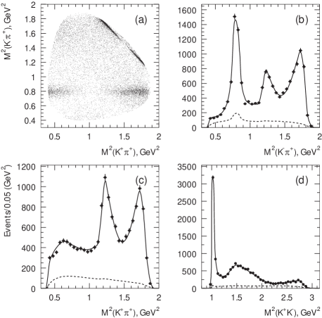
Figure 1: The results of fitting the $D^{+}\to K^{+}K^{-}\pi^{+}$ data for Model three. (a) The scatter plot for squared mass of $K^{-}\pi^{+}$ versus $K^{+}\pi^{+}$ and the projections onto squared mass of (b) $K^{-}\pi^{+}$ (c) $K^{+}\pi^{+}$ and (d) $K^{+}K^{-}$ for both fit (curve) and data (points) are shown. The dashed line shows the background contribution.

Table 1: The fit results in Model three. The errors shown are statistical, experimental systematic, and modeling systematic respectively.

Component	Amplitude	Phase (∘)	Fit Fraction (%)
$\overline{K}^{*}(892)^{0}K^{+}$	1(fixed)	0(fixed)	$23.9\pm 0.6^{+0.1+0.9}_{-0.3-0.4}$
$K^{-}\pi^{+}(S)K^{+}$	$4.53\pm 0.16^{+0.22+0.31}_{-0.01-0.23}$	$21\pm 3^{+0+7}_{-6-2}$	$53\pm 3^{+5+8}_{-0-5}$
$a_{0}(980)\pi^{+}$	$0.74\pm 0.09^{+0.03+0.16}_{-0.01-0.39}$	$96\pm 7^{+0+4}_{-4-15}$	$1.7\pm 0.4^{+0.1+1.3}_{-0.0-0.6}$
$\phi(1020)\pi^{+}$	$1.23\pm 0.02^{+0.00+0.01}_{-0.00-0.02}$	$-148\pm 3^{+1+5}_{-1-3}$	$28.0\pm 0.5^{+0.0}_{-0.4}\pm 0.5$
$f_{2}(1270)\pi^{+}$	$0.91\pm 0.13_{-0.01-0.24}^{+0.03+0.11}$	$20\pm 6^{+5+9}_{-0-11}$	$0.9\pm 0.2^{+0.1}_{-0.0}\pm 0.2$
$a_{0}(1450)\pi^{+}$	$1.36\pm 0.10^{+0.20+0.45}_{-0.01-0.25}$	$116\pm 5^{+1+13}_{-5-10}$	$3.4\pm 0.5^{+1.0+2.5}_{-0.0-1.2}$
$\phi(1680)\pi^{+}$	$2.6\pm 0.3^{+0.2+0.6}_{-0.0-0.7}$	$-96\pm 10^{+0+17}_{-16-12}$	$0.89\pm 0.18^{+0.15+0.3}_{-0.02-0.2}$
$\overline{K}_{2}^{*}(1430)^{0}K^{+}$	$3.5\pm 1.0^{+1.6+1.6}_{-0.0-2.6}$	$-156\pm 6_{-0-8}^{+1+30}$	$2.1\pm 1.2^{+2.4+2.2}_{-0.0-1.3}$

We determine the detection efficiency as a function of the two DP variables by fitting a signal MC sample generated with a flat distribution in the phase space. We use a fit to the events in the $\Delta E$ sideband ($24<|\Delta E|<42$ MeV and $|m_{\rm BC}-m_{D^{+}}|<9$ MeV/$c^{2}$) to describe the background distribution of the DP. Having information for both the background and efficiency, as well as the fraction of signal events in the signal region, we fit the data in the DP to extract the amplitudes and phases of any contributing intermediate resonances. We perform an unbinned maximum likelihood fit. The signal fraction $f$ is $f_{0}=(84.1\pm 0.2$)%, constrained in the fit to be within its error $\sigma_{f}$ obtained from the fit to the $m_{\rm BC}$ distribution. We begin by fitting the DP with all known resonances that may possibly contribute to this decay. We determine which resonances are to be included by maximizing the fit confidence level (C.L.). The procedure is to add all possible resonances, then subsequently remove those which do not contribute significantly, or worsen our C.L. The projections of the DP for the fit to Model three are shown in Figures 1(b-d). The results of the fit amplitudes, phases, and fractions including errors are shown in Table 1 for Model three.

Table 2: $A_{CP}$ for each component of the fit using $D^{\pm}$ samples in Model three. The errors for fit fractions and phases are statistical only, and those for $A_{CP}$ are statistical, experimental systematic, and modeling systematic respectively.

Component $j$	${A_{CP}}_{j}$(%)
$\overline{K}^{*}(892)^{0}K^{+}$	$-0.1\pm 2.9_{-0.4-0.4}^{+2.3+0.7}$
$K^{-}\pi^{+}(S)K^{+}$	$-1\pm 5_{-2-4}^{+1+6}$
$a_{0}(980)\pi^{+}$	$-11\pm 23_{-9-6}^{+4+24}$
$\phi(1020)\pi^{+}$	$-3.0\pm 1.9_{-0.2-0.3}^{+0.1+0.2}$
$f_{2}(1270)\pi^{+}$	$4\pm 25_{-4-46}^{+3+22}$
$a_{0}(1450)\pi^{+}$	$-18\pm 14_{-8-9}^{+0+16}$
$\phi(1680)\pi^{+}$	$-9\pm 21_{-4-3}^{+22+7}$
$\overline{K}_{2}^{*}(1430)^{0}K^{+}$	$69\pm 51_{-28-41}^{+1+8}$

To search for $CP$ violation in this model, we fit the $D^{+}$ and $D^{-}$ samples independently. We use the same background fraction and PDF as those used in the fit to the total sample, but different coefficients for efficiency functions which are obtained from signal MC of $D^{\pm}$ decays. The calculated $CP$ asymmetry, ${A_{CP}}_{j}\equiv\frac{{FF_{j}}_{D^{+}}-{FF_{j}}_{D^{-}}}{{FF_{j}}_{D^{+}}+{FF_{j}}_{D^{-}}}$, is shown for each resonance $j$ in Table 2.

2 Dalitz Plot Analysis of $D^{0}\to K^{0}_{S}\pi^{0}\pi^{0}$ Decays

The PDG [11] has little information on the $D^{0}\rightarrow K^{0}_{S}\pi^{0}\pi^{0}$ decay. In addition to providing a more comprehensive study of the $D^{0}\rightarrow K^{0}_{S}\pi^{0}\pi^{0}$ decay, this DP analysis seems like a good place to look for the low mass $\pi\pi$ $S$-wave signature of the $\sigma$. The $K^{0}_{S}\pi^{+}\pi^{-}$ mode is much cleaner and has better statistics, but the $\rho^{0}$ resonance overlaps the region where we would expect to find the low mass $S$-wave signature. Using CLEO-c data, we eliminate nearly all of the background by doing a double-tagged analysis, where both $D$ mesons are completely reconstructed.

We have analyzed $281$ pb^-1 of CLEO-c data taken on the $e^{+}e^{-}\to\psi(3770)$ resonance. In a double-tagged analysis, both $D$ mesons are reconstructed. For our double-tagged analysis, we consider candidates with one $D$ reconstructed as $K^{0}_{S}\pi^{0}\pi^{0}$, and the other $D$ reconstructed using any of the following decay modes (charge conjugation is implied throughout this analysis): $\overline{D^{0}}\rightarrow K^{+}\pi^{-}$, $\overline{D^{0}}\rightarrow K^{+}\pi^{-}\pi^{0}$, $\overline{D^{0}}\rightarrow K^{+}\pi^{-}\pi^{+}\pi^{-}$. In a single-tagged analysis, we reconstruct only one $D$ meson in the event, which decays to $K^{0}_{S}\pi^{0}\pi^{0}$.

Table 3: $D^{0}\rightarrow K^{0}_{S}\pi^{0}\pi^{0}$ signal yield, number of candidates, and signal fraction

Result	Double Tag	Single Tag
Signal Yield	257 $\pm$ 17	1884 $\pm$ 56
Total Candidates	276	2548
Signal Fraction	0.931 $\pm$ 0.062	0.739 $\pm$ 0.022

To reduce $2\pi$ background that fakes a $K^{0}_{S}$, we enforce a $2\sigma$ enhanced flight significance selection criteria on our $K^{0}_{S}$ candidates. To reduce the $K\pi\pi^{0}$ background, we require $|dE/dx_{pion}|$ $<$ $3\sigma$ and $dE/dx_{kaon}$ $<$ $-2\sigma$ for both $K^{0}_{S}$ daughter pions. We use the same particle identification selection criteria for double-tagged and single-tagged analyses. We apply a $2\sigma$ selection criteria on the reconstructed $K^{0}_{S}$ mass. After enforcing our selection criteria on the $K^{0}_{S}$ mass, we apply a $2\sigma$ selection criteria on $\Delta E$. We additionally apply a $2\sigma$ cut on the beam constrained mass. For each event that has more than one candidate, we require the following: For the double-tagged data, we take the average of the signal beam constrained mass and the tagged beam constrained mass, and we select whichever candidate’s average is closest to the nominal $D$ mass. For the single-tagged data, we select the candidate with $\Delta E$ closest to zero. Table 3 shows our signal yield and signal fraction.

For this analysis, we define our DP variables as follows: $x$ $\equiv$ larger $m_{K^{0}_{S}\pi^{0}}^{2}$, $y$ $\equiv$ $m_{\pi^{0}\pi^{0}}^{2}$, $z$ $\equiv$ smaller $m_{K^{0}_{S}\pi^{0}}^{2}$. When fitting such a Dalitz plot, we must take into account the fact that the two $\pi^{0}$ final state particles are indistinguishable, so we explicitly symmetrize the functions we use in $x$ and $z$.

To study the efficiency of reconstructing our signal, we generate 100000 signal Monte Carlo events distributed uniformly across the Dalitz plot phase space. Half of these events force the $D^{0}$ to decay directly into $K^{0}_{S}\pi^{0}\pi^{0}$ and the $\overline{D}^{0}$ to decay into neutrinos. The other half of these events force the $\overline{D}^{0}$ to decay directly into our signal mode and the $D^{0}$ to decay into neutrinos. We fit the efficiency over the Dalitz plot to a third-order polynomial explicitly symmetric in $x$ and $z$. To fit for the background, we use a sideband from single-tagged data which is centered 5$\sigma_{m_{D^{0}}}$ lower in $m_{BC}$ than the signal region, with the same width as that of the signal region, and has the appropriate range in $\Delta{E}$ which conserves the boundaries of the signal DP. We use this background shape for the double-tagged data as well as for the single-tagged data. We fit the background events to a third-order polynomial explicitly symmetric in $x$ and $z$, plus a non-interfering $K^{*}(892)$ Breit-Wigner in both $x$ and $z$.

The signal is parameterized with an isobar model that has four interfering resonances plus one non-interfering resonance. To enforce the symmetry requirement in the DP, we include each $K^{*}$ resonance as an $x$ resonance and a $z$ resonance, while using the same amplitude and phase for the $x$ contribution and $z$ contribution. The parameters for the $K^{0}_{S}$, $K^{*}(892)$, and $K^{*}(1680)$ come from the PDG [11]. The parameters for the $f_{0}(980)$ are approximated from a BES paper [12]. The parameters for the $f_{0}(1370)$ come from Reference [13].

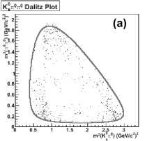
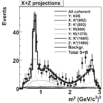
Figure 2: (a) Dalitz plot of the double-tagged data (2 entries per candidate, second entry has $x$ and $z$ swapped) and (b) fits to the double-tagged x+z projection and double-tagged y projection.

Figure 2(a) displays the DP from the double-tagged data. To fit this DP with an unbinned maximum likelihood fitter, we fix the signal fraction to 0.931 as determined from the beam constrained mass distribution. The fit also fixes the efficiency parameters and background parameters as determined from the signal Monte Carlo and sideband. The fit determines the amplitudes and phases of the resonances and calculates the fit fractions. Figure 2(b) shows the fit results.

Table 4: Final results including systematic errors. The first error is statistical. The second error is systematic arising from our selection criteria. The third error is systematic arising from our signal model.

resonance		double tag
	Fit Fraction	$0.026\pm 0.023\pm 0.003\pm 0.001$
$K^{0}_{S}$	Amplitude	$0.101\pm 0.029\pm 0.009\pm 0.004$
	Effective Width	$0.0046\pm 0.0011\pm 0.0001\pm 0.0001$
	Fit Fraction	$0.542\pm 0.054\pm 0.030\pm 0.053$
$K^{*}(892)$	Amplitude	$1$ (fixed)
	Phase (∘)	$0$ (fixed)
	Fit Fraction	$0.090\pm 0.032\pm 0.009\pm 0.027$
$f_{0}(980)$	Amplitude	$1.50\pm 0.27\pm 0.10\pm 0.20$
	Phase (∘)	$12\pm 17\pm 14\pm 8$
	Fit Fraction	$0.238\pm 0.071\pm 0.047\pm 0.086$
$f_{0}(1370)$	Amplitude	$2.77\pm 0.45\pm 0.30\pm 0.66$
	Phase (∘)	$344\pm 10\pm 10\pm 18$
	Fit Fraction	$0.114\pm 0.027\pm 0.021\pm 0.032$
$K^{*}(1680)$	Amplitude	$4.55\pm 0.68\pm 0.49\pm 0.59$
	Phase (∘)	$97\pm 20\pm 17\pm 13$

To estimate systematic errors, we use the technique developed by Jim Wiss and Rob Gardner [14]. Using this technique, the systematic errors are essentially independent of the number of systematic sources considered [14]. Table 4 gives our preliminary results. We are currently extending our analysis to the full available CLEO-c $\psi(3770)$ data sample, and studying the effects of using a $\sigma$ or $\kappa$ $S$-wave to possibly improve our fit.

3 Acknowledgements

We would like to thank David Asner, David Cinabro, Mikhail Dubrovin, Qing He, Mats Selen, Ed Thorndike, Eric White, our paper committees, and the rest of the CLEO-c Dalitz Plot Analysis Working Group for their insight, comments, and suggestions.

4 References

References

- 1 . M. Dubrovin et al, Phys. Rev. D 76, 012001 (2007).
- 2 . M. Dubrovin, hep-ex/0707.3060 (2007)
- 3 . E.J. White and Q. He, hep-ex/0711.2285 (2007)
- 4 . Y. Grossman, A. L. Kagan, Y. Nir, Phys. Rev. D 75, 036008 (2007).
- 5 . S. Kopp et al. (CLEO Collaboration), Phys. Rev. D 63, 092001 (2001).
- 6 . E. M. Aitala et al. (E791 Collaboration), Phys. Rev. Lett. 86, 765 (2001).
- 7 . A. Abele et al., Phys. Rev. D 57, 3860 (1998).
- 8 . P. L. Frabetti et al. (E687 Collaboration), Phys. Lett. B 351, 591 (1995).
- 9 . D. Aston et al. (LASS Collaboration), Nucl. Phys. B 296, 493 (1988).
- 10 . B. Aubert et al. (BABAR Collaboration), Phys. Rev. D 76, 011102(R) (2007).
- 11 . W. M. Yao et al. (Particle Data Group Collaboration), Journal of Physics G 33, 1 (2006) and 2007 partial update for edition 2008.
- 12 . M. Ablikim, et al., BES Collab., Phys. Lett. B 607 (2005) 243.
- 13 . A. Kirk, hep-ph/0009168 (2000).
- 14 . Jim Wiss, Rob Gardner, “Estimating Systematic Errors”, unpublished (1994).