Decomposition During Search for Propagation-Based Constraint Solvers

Abstract

We describe decomposition during search (DDS), an integration of And/Or tree search into propagation-based constraint solvers. The presented search algorithm dynamically decomposes sub-problems of a constraint satisfaction problem into independent partial problems, avoiding redundant work.

The paper discusses how DDS interacts with key features that make propagation-based solvers successful: constraint propagation, especially for global constraints, and dynamic search heuristics.

We have implemented DDS for the Gecode constraint programming library. Two applications, solution counting in graph coloring and protein structure prediction, exemplify the benefits of DDS in practice.

1 Introduction

Propagation-based constraint solvers owe much of their success to a best-of-several-worlds approach: They combine classic AI search methods with advanced implementation techniques from the Programming Languages community and efficient algorithms from Operations Research. Furthermore, the CP community has developed a great number of propagation algorithms for global constraints.

In this paper, we present how to integrate And/Or search into propagation-based constraint solvers. We call the integration decomposition during search (DDS). We take full advantage of all the features mentioned above that make propagation-based constraint solvers successful. The most interesting points, and main contributions of our paper, are how DDS interacts with and benefits from constraint propagation, especially in the presence of global constraints, and dynamic search heuristics. We exemplify the profit of DDS by exhaustive solution counting, an important application area of decomposing search strategies [3, 8].

Related work. Only recently, counting and exhaustive enumeration of solutions of a constraint satisfaction problem (CSP) gained a lot of interest [1, 3, 8, 21]. In general, the counting of CSP solutions is in the complexity class #P, i.e. it is even harder than deciding satisfiability [19]. This class was defined by Valiant [24] as the class of counting problems that can be computed in nondeterministic polynomial time. Notwithstanding the complexity, there is demand for solution counting in real applications. For instance, in bioinformatics counting optimal protein structures is of high importance for the study of protein energy landscapes, kinetics, and protein evolution [20, 25] and can be done using CP [2].

Already folklore, standard solving methods for CSPs like Depth-First Search (DFS) leave room for saving redundant work, in particular when counting all solutions [10]. Recent work by Dechter et al. [8, 15] introduced And/Or search for solution counting and optimization, which makes use of repeated and-decomposition during the search following a pseudo-tree. Their work thoroughly studies and develops a rich theory of And/Or trees.

While not in the context of general constraint propagation, similar ideas were discussed before for SAT-solving [3, 5, 14]. The SAT approaches also introduce the idea of analyzing the induced dependency structure dynamically during the search. This avoids redundancy that occurs due to the emergence of independent connected components in the dependency graph during the search.

Motivation and contribution. The motivation for this paper is to tackle the same kind of redundancy for solving very hard real world problems, such as the counting of protein structures, that require a full-fledged constraint programming system. This requests for a method which is tailored for integration into modern CP systems and directly supports features such as global constraints and dynamic search heuristics. To make use of the statically unpredictable effects of constraint propagation and entailment, the presented method avoids redundant search dynamically.

Our main contribution is to present how to integrate And/Or tree search into a state-of-the-art, propagation-based constraint solver. This is exemplified by extending the Gecode system [11]. We describe decomposition during search (DDS) on different levels of abstraction, down to concrete implementation details.

In detail, we stress the impact that constraint propagation has on decomposability of the constraint graph, and how DDS interacts (and works seamlessly together) with propagators for global constraints, the workhorses of modern propagation-based solvers. We show that global constraint decomposition is the key to enable the application of DDS, and discuss techniques that enable global constraint decomposition. The practical value of DDS in the presence of global constraints is shown empirically, using a well integrated and competitive implementation for the Gecode library.

Overview. The paper starts with a presentation of the notations and concepts that are used throughout the later sections. In Sec. 3, we briefly recapitulate And/Or search, and then present, on a high level of abstraction, decomposition during search (DDS), our integration of And/Or search into a propagation-based constraint solver. Sec. 4 deals with the interaction of DDS with propagation and search heuristics. Section 5 discusses how global constraints interact with DDS, focusing on decomposition strategies for some important representatives.

On a lower level of abstraction, Sec. 6 sketches the concrete implementation of DDS using the Gecode C++ constraint programming library. With the help of our Gecode implementation, we study the practical impact of DDS in Sec. 7 by counting solutions for random instances of two important CSPs, graph coloring and protein structure prediction. Both examples are hard counting problems (in class #P). The study shows high average speedups and reductions in search tree size, even using our prototype implementation. These two sections therefore provide evidence that DDS can be integrated into a modern constraint programming system in a straightforward and efficient way. The paper finishes with a summary and an outlook on future work in Sec. 8.

2 Preliminaries

This section defines the central notions that we want to use to talk about constraint satisfaction problems.

A Constraint Satisfaction Problem (CSP) is a triple $P=({\mathcal{X}},{\mathcal{D}},{\mathcal{C}})$, where ${\mathcal{X}}=\{x_{1},\ldots,x_{m}\}$ is a finite set of variables, ${\mathcal{D}}$ a function of variables to their associated value domains, and ${\mathcal{C}}$ a set of constraints. An $n$-ary constraint $c\in{\mathcal{C}}$ is defined by the tuple of its $n$ variables $\operatorname{vars}(c)$ and a set of $n$-tuples of the allowed value combinations. We feel free to interpret $\operatorname{vars}(c)$ as the set of variables of $c$. A domain ${\mathcal{D}}$ entails a constraint $c$ if and only if all possible value combinations of the variable domains of $\operatorname{vars}(c)$ in ${\mathcal{D}}$ are allowed tuples for $c$. A solution of a CSP is an assignment of one value $v\in{\mathcal{D}}(x_{i})$ to each variable $x_{i}\in{\mathcal{X}}$ such that all $c\in{\mathcal{C}}$ are entailed. The set of solutions of a CSP $P$ is denoted by $\operatorname{sol}(P)$.

Based on these definitions some important properties of a CSP can be defined. A CSP $P=({\mathcal{X}},{\mathcal{D}},{\mathcal{C}})$ is solved if and only if $\forall x\in{\mathcal{X}}:|{\mathcal{D}}(x)|=1$ and $\operatorname{sol}(P)\neq\emptyset$. P is failed if and only if $\operatorname{sol}(P)=\emptyset$ and satisfiable otherwise. A CSP $P^{\prime}$ is stronger than $P$ ($P^{\prime}\sqsubseteq P$) if and only if $\operatorname{sol}(P^{\prime})=\operatorname{sol}(P)$ and $\forall x\in{\mathcal{X}}^{\prime}:{\mathcal{D}}^{\prime}(x)\subseteq{\mathcal{D}}(x)$.

The constraint graph of a CSP $P=({\mathcal{X}},{\mathcal{D}},{\mathcal{C}})$ is a hypergraph $G_{P}=(V,E)$, where $V={\mathcal{X}}$ and $E=\{\operatorname{vars}(c)\mid c\in{\mathcal{C}}\}$.

3 Decomposition During Search

In this section, we recapitulate And/Or tree search. Then, we present a high-level model of how to integrate And/Or tree search into a propagation-based constraint solver. We call this integration decomposition during search (DDS).

3.1 And/Or tree search

Let us look at an example to get an intuition for And/Or search. Assume $P=({\mathcal{X}},{\mathcal{D}},{\mathcal{C}})$ with ${\mathcal{X}}=\{A,B,C,D\}$, ${\mathcal{D}}(A)=\{3,5\}$, ${\mathcal{D}}(B)=\{3,4\}$, ${\mathcal{D}}(C)={\mathcal{D}}(D)=\{1,2\}$, and ${\mathcal{C}}=$ ‘$A,B,C,D$ are pairwise different’. Figure 1 presents a corresponding search tree for a plain depth-first tree search. Each node is a propagated sub-problem of $P$ and is visualized as a constraint graph. As usual, a node is equivalent to the disjunction of all its children.

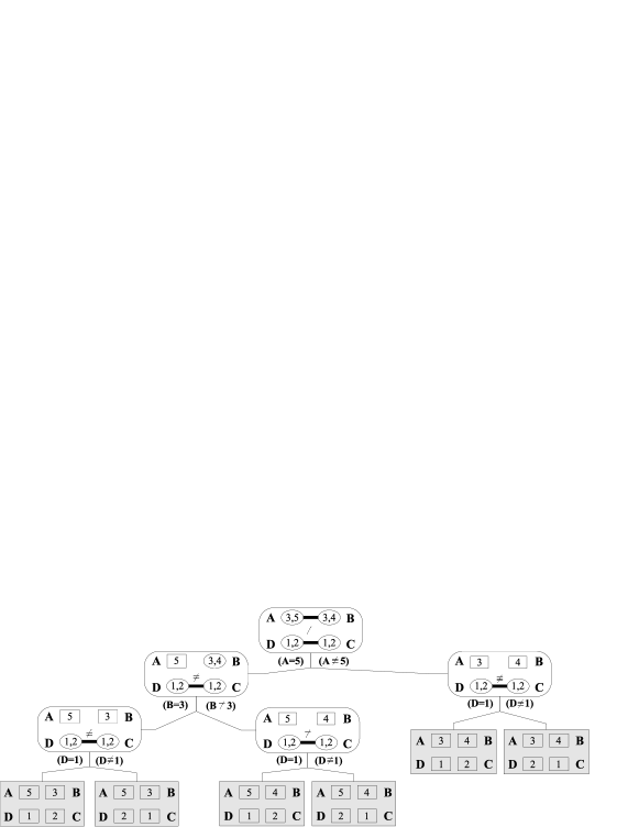
Figure 1: DFS search tree.

Even this tiny example demonstrates that plain DFS may perform redundant work: The partial problem on the variables $C$ and $D$ is solved redundantly for each solution of the partial problem on $A$ and $B$. We say that $\{A,B\}$ and $\{C,D\}$ are independent sets of variables.

The central idea of And/Or tree search [8] is to detect independent partial problems during search, to enumerate partial solutions of the partial problems independently, and finally to combine them to solutions, or to compute the number of solutions. That way, each independent partial problem is searched only once. The name And/Or search stresses that the search tree contains both disjunctive, choice nodes (OR) and conjunctive nodes (AND), representing decompositions. Figure 2 shows a search tree for the same CSP as in Figure 1, but using And/Or search. For now, you can read the big $X$ as “combine”. Here, the search tree contains only one decomposition and two choices, instead of five choices in Figure 1. In general, the amount of redundant work can be exponential in the size of the CSP.

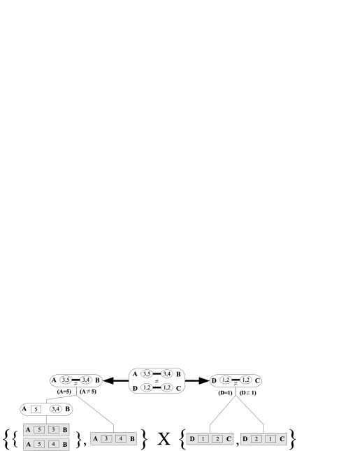
Figure 2: And/or search tree.

3.2 Integrating And/Or search into a propagation-based solver

From a bird’s eye view, And/Or search can be done easily in the context of propagation-based constraint solving. Algorithm 1 counts all solutions of a CSP $P$, decomposing the problem where possible.

Ignoring line 5 for a moment, the algorithm runs a standard depth-first search (DFS). The function Propagate in line 2 performs constraint propagation: it maps a CSP $P=({\mathcal{X}},{\mathcal{D}},{\mathcal{C}})$ to a CSP $P^{\prime}=({\mathcal{X}},{\mathcal{D}}^{\prime},{\mathcal{C}}^{\prime})$ such that $P^{\prime}\sqsubseteq P$. Propagate may remove entailed constraints from ${\mathcal{C}}$. If $P^{\prime}$ is failed or solved, we just return that we found no resp. one solution (lines 3,4). Otherwise (line 6), we split the problem into LeftChoice($P^{\prime}$) and RightChoice($P^{\prime}$). These functions implement the search heuristic and will be discussed in more detail in Sec. 4.2. As the branches correspond to a disjunction of $P^{\prime}$, the recursive counts add up to the total number of solutions.

Algorithm 1 Counting by Decomposition During Search

1:function DDS($P$)

2:    $P^{\prime}\leftarrow$ Propagate($P$)

3:    if IsFailed($P^{\prime}$) return 0

4:    if IsSolved($P^{\prime}$) return 1  

5:    if Decompose($P^{\prime}$)$=(P^{\prime}_{1},P^{\prime}_{2})$  return  DDS($P^{\prime}_{1}$) $\cdot$ DDS($P^{\prime}_{2}$)

6:$\triangleright$ decomposition

7:    return  DDS(LeftChoice($P^{\prime}$))  +  DDS(RightChoice($P^{\prime}$))

8:$\triangleright$ choice

9:end function

The only addition that is necessary to turn DFS into an And/Or search is line 5: If the problem can be decomposed into $P^{\prime}_{1}$ and $P^{\prime}_{2}$ (we simplify by assuming only binary decomposition), these partial problems in conjunction are equivalent to $P^{\prime}$. Hence, we multiply the results of the recursive calls.

In contrast to investigating decomposability only on the initial CSP for a static variable selection, Algorithm 1 follows a dynamic approach: the check for decomposability is interleaved with propagation and normal search. As search progresses, more and more variables are assigned to values, and more and more constraints are detected to be entailed. We shall see that this greatly increases the potential for decomposition in Sec. 4. Furthermore, decomposition is completely independent of the implementation of LeftChoice and RightChoice, so any search heuristic can be used.

Short-circuit. As a straightforward optimization, we can employ short-circuit reasoning in line 5. If $\textsc{DDS}(P^{\prime}_{1})$ returns no solutions, we do not have to compute $\textsc{DDS}(P^{\prime}_{2})$ at all. Note the potential pitfall here: There are situations where DFS detects failure easily, but DDS has to search a huge partial problem $P^{\prime}_{1}$ before detecting failure in $P^{\prime}_{2}$. We come back to this in Sec. 4.2.

Enumerating solutions. Extending DDS to enumeration of solutions is straightforward: We just have to return an empty list in case of failure (line 3), a singleton list with a solution when we find one (line 4), and interpret addition as list concatenation and multiplication as combination of partial solutions. Instead of enumeration, we can also build up a tree-shaped compact representation of the solution space (as in Fig. 2 and later in Fig. 9c).

In the rest of this section, we show how to compute the Decompose function efficiently.

3.3 Computing the decomposition

We will now define formally when a CSP can be decomposed, and give a sufficient algorithmic characterization that leads to an efficient implementation.

Restriction and independence. The restriction of a function $f:{\mathcal{Y}}\rightarrow{\mathcal{Z}}$ to a set ${\mathcal{X}}\subseteq{\mathcal{Y}}$ is defined as

$${f}_{|{\mathcal{X}}}:{\mathcal{X}}\rightarrow{\mathcal{Z}},x\mapsto f(x).$$

We define the restriction of a CSP $P=({\mathcal{X}},{\mathcal{D}},{\mathcal{C}})$ to a set of variables ${\mathcal{X}}^{\prime}\subseteq{\mathcal{X}}$ by ${P}_{|{\mathcal{X}}^{\prime}}=({\mathcal{X}}^{\prime},{{\mathcal{D}}}_{|{\mathcal{X}}^{\prime}},{{\mathcal{C}}}_{|{\mathcal{X}}^{\prime}})$, where

$${{\mathcal{C}}}_{|{\mathcal{X}}^{\prime}}=\{c\in{\mathcal{C}}\mid\operatorname{vars}(c)\subseteq{\mathcal{X}}^{\prime}\}.$$

A non-empty proper subset $\hat{\mathcal{X}}\subset{\mathcal{X}}$ is independent in a CSP $P=({\mathcal{X}},{\mathcal{D}},{\mathcal{C}})$, if and only if

$$\operatorname{sol}(P)=\emptyset\text{ or }{\operatorname{sol}(P)}_{|\hat{\mathcal{X}}}=\operatorname{sol}({P}_{|\hat{\mathcal{X}}}).$$

For $\hat{\mathcal{X}}$ independent in $P$, we say that ${P}_{|\hat{\mathcal{X}}}$ is a partial problem of $P$. We can decompose $P$ if it has a partial problem.

The key to an efficient implementation of Decompose is to have an algorithmic interpretation of what it means that a CSP can be decomposed into partial problems. We now show that connected components in the constraint graph of a CSP represent independent partial problems.

A graph is connected if and only if there exists a path between all nodes. A connected component of a constraint graph $G_{P}$ is a maximal connected subgraph.

Proposition 1

Consider a CSP $P=({\mathcal{X}},{\mathcal{D}},{\mathcal{C}})$ with constraint graph $G_{P}$. If $\hat{\mathcal{X}}\subset{\mathcal{X}}$ is a connected component in $G_{P}$, then ${P}_{|\hat{\mathcal{X}}}$ is a partial problem of $P$.

Proof

There exists no hyperedge between node $x\in\hat{\mathcal{X}}$ and node $y\notin\hat{\mathcal{X}}$, as connected components are maximal. This means that there is no constraint between any $x$ and $y$ in $P$. We have to distinguish two cases: If $P$ is unsatisfiable, $\hat{\mathcal{X}}$ is trivially independent (by definition of independence). Otherwise, take an arbitrary solution $\hat{s}\in\operatorname{sol}({P}_{|\hat{\mathcal{X}}})$, and an arbitrary solution $s\in\operatorname{sol}(P)$. Merging $\hat{s}$ into $s$ yields $s^{\prime}=(x\mapsto\hat{s}(x)$ for $x\in\hat{\mathcal{X}}$, $x\mapsto s(x)$ otherwise). This $s^{\prime}$ is again a solution of $P$, as all constraints on ${\mathcal{X}}\setminus\hat{\mathcal{X}}$ are still satisfied, and all constraints on $\hat{\mathcal{X}}$ are satisfied, too. As we picked $s$ and $\hat{s}$ arbitrarily, we get ${\operatorname{sol}(P)}_{|\hat{\mathcal{X}}}\supseteq\operatorname{sol}({P}_{|\hat{\mathcal{X}}})$. Because ${C}_{|\hat{\mathcal{X}}}$ of ${P}_{|\hat{\mathcal{X}}}$ covers all constraints of ${\mathcal{C}}$ restricting $\hat{\mathcal{X}}$, it follows ${\operatorname{sol}(P)}_{|\hat{\mathcal{X}}}\subseteq\operatorname{sol}({P}_{|\hat{\mathcal{X}}})$.
Therefore, it holds ${\operatorname{sol}(P)}_{|\hat{\mathcal{X}}}=\operatorname{sol}({P}_{|\hat{\mathcal{X}}})$.

This result is not new [3, 10], but we repeat it to illustrate the central algorithmic idea. Connected components can be computed in linear time in the size of the graph, and incremental algorithms are available. We can thus implement Decompose as a simple connectedness algorithm on the constraint graph that yields all partial problems of the current CSP.

Finding more than one non-empty connected component is a sufficient condition for finding partial problems, but not a necessary one. As an example, consider the CSP that contains the trivial constraint allowing all combinations of values for $x$ and $y$. Then $x$ and $y$ may still be independent, but the constraint graph shows a hyperedge connecting the two variables, so that $x$ and $y$ will always end up in the same connected component. In the following section, we will see how propagation-based solvers can deal with this.

4 How DDS Interacts With Propagation and Search

The previous section showed how DDS can be integrated into a propagation-based solver. But what are the consequences, how is decomposition affected by propagation and search, and how can it benefit from the search heuristic?

4.1 Constraint graph dynamics

Decomposition examines the constraint graph during search. This is vital as propagation and search modify the constraint graph dynamically – they narrow the domains of the problem’s variables and remove some entailed constraints. The result is a sparser constraint graph with more potential for decomposition:

Assignment. Clearly, an assigned variable ($|{\mathcal{D}}(x)|=1$) is independent of all other variables of the CSP. This implies that connections of hyperedges to assigned variables can be removed from the constraint graph – the constraint graph becomes sparser. Assignment increases the potential for decomposition, since an assigned variable may have been responsible for keeping two otherwise independent parts of the graph connected.

Entailment. Consider the example CSP $P=({\mathcal{X}},{\mathcal{D}},{\mathcal{C}})$ from the end of the previous section, where variables $x\in{\mathcal{X}}$ and $y\in{\mathcal{X}}$ are connected by a trivial constraint $c\in{\mathcal{C}}$ allowing all possible value tuples. Obviously, $c$ is entailed in $P$, it will not contribute to propagation any more. Formally, we have for $P^{\prime}=({\mathcal{X}},{\mathcal{D}},{\mathcal{C}}\setminus\{c\})$ that $\operatorname{sol}(P^{\prime})=\operatorname{sol}(P)$. It is also obvious that the constraint graph for $P^{\prime}$ is sparser than the one for $P$, it contains one edge less. It is thus vital to our approach to detect entailment of constraints as early as possible, and to remove entailed constraints from ${\mathcal{C}}$. Clearly, full entailment detection is coNP-complete. Most CP systems (e.g. Gecode) however implement a weak form of entailment detection in order to remove propagators early, which our approach automatically benefits from.

4.2 Search heuristics

The applied search heuristic, encoded by LeftChoice and RightChoice, is extremely important for the efficiency of the search. In particular, dynamic heuristics, natively supported by DDS, are known to be largely superior to static ones.

In the following (and for our implementation) we refer to the common variable-value heuristics that select a variable $x$ and a value $v\in{\mathcal{D}}(x)$. Afterwards, the disjunction is done by $\textsc{LeftChoice}(P)=({\mathcal{X}},{\mathcal{D}},{\mathcal{C}}\cup(x\diamond v))$ and $\textsc{RightChoice}(P)=({\mathcal{X}},{\mathcal{D}},{\mathcal{C}}\cup\lnot(x\diamond v))$, where $\diamond$ is some binary relation.

Variable selection. The variable selection strategy of such a heuristic is crucial for the size of the search tree and often problem specific. Nevertheless, a common method for variable selection is ‘first-fail’, which selects by minimal domain size. Other strategies use the degree in the constraint graph or the minimal/maximal/median value in the domain. Static variable orderings are in many cases inferior to these dynamic strategies. To gain the best search performance by DDS, the variable selection further has to induce constraint graph decompositions as early as possible.

Heuristics that maximize decomposition. In order to maximize the number of decompositions during search, the heuristic can be guided by the constraint graph. Such a heuristic may compute e.g. cut-points, bridges, or more powerful (minimal) cut-sets/separators [16]. Our framework is well prepared to accommodate such complex strategies, in particular because our method already builds on access to the constraint graph.

An open problem is the possible contradiction of heuristics aimed at decomposition versus fine-tuned problem specific heuristics. The heuristic aimed at decomposition may yield many partial problems that are not satisfiable and therefore lead to an inefficient search. On the other hand, the problem specific heuristic might yield no or only a few decompositions, which makes DDS unprofitable. Therefore, no general rule can be given. But our experiments suggest that a hybrid heuristic of selecting the variable with the highest node degree, and using the problem-specific heuristic as a tie breaker, yields good results (see Sec. 7).

Order of exploration of partial problems. It is of high importance in which order the children of and-nodes, the partial problems, are explored. After detecting inconsistency in one partial problem, the exploration of the remaining partial problems is needless. Given an unsatisfiable problem, a good variable selection heuristic yields a failure during search as soon as possible to avoid unnecessary search (this is called the fail-first principle). Assuming that we already have such a good variable selection heuristic, we use it to guide the partial problem ordering of DDS: (1) apply the selection to the whole (non-decomposed) variable set and (2) choose the partial problem first that contains the selected variable. That way, a good heuristic will lead to failure in the first explored partial problem if the decomposed problem has no solution. Further, it decreases the probability that the remaining partial problems are not satisfiable (in case the first is). This mitigates the effect that failure may be detected late using DDS, mentioned in Subsec. 3.2.

5 Global Constraints

One of the key features of modern constraint solvers is the use of global constraints to strengthen propagation. Therefore, a search algorithm has to support global constraints in order to be practically useful in such systems. We describe the problems global constraints pose for DDS, and how to tackle them.

For an $n$-ary (global) constraint, the constraint graph contains a hyperedge that connects all $n$ variable nodes. Consider a CSP for $\textsf{All-different}(w,x,y,z)$ with $w,x\in\{0,1\}$, $y,z\in\{2,3\}$. In this model, we cannot decompose, although the binary constraints $a\neq b$ for $a\in\{w,x\}$, $b\in\{y,z\}$ are entailed! Thus, in the current set-up, the global All-different unnecessarily prevents decomposition.

The solution to this problem is to take the internal structure of global constraints into account: the global constraint itself can be decomposed into smaller constraints (on fewer variables). We will call this the constraint decomposition to distinguish it from constraint graph decomposition.

If we reflect the constraint decomposition of global constraints in the constraint graph, we recover all the decompositions that were prevented by the global constraints before.

For our example involving the All-different constraint, the constraint graph would contain two constraints, $w\neq x$ and $y\neq z$, instead of the one global All-different. The graph can now be decomposed.

As global constraints often cover a significant portion of the variables in a problem, global constraint decomposition is an essential prerequisite to make a constraint graph decomposition by DDS possible. Note that global constraint decomposition is independent of the other constraints present in the constraint graph; typical permutation problems, for instance, feature one global All-different that forces all variables to form a permutation, and then several other constraints that determine the concrete properties of the permutation. Applying DDS to such a problem is useless unless the constraint decomposition of the All-different is considered when computing connected components.

In general, a global constraint can be decomposed if and only if its extension (the set of allowed tuples) can be represented as a non-trivial product, i.e. a product of non-singleton sets. For the above example, the set of allowed tuples is $\{(0,1),(1,0)\}\times\{(2,3),(3,2)\}$. If a constraint can be represented as such a non-trivial product $a\times b$, we can decompose it into two independent constraints, one with the tuples of $a$, the other with the tuples of $b$.

Formally, defined in terms of CSP solutions, we say a constraint $c\in{\mathcal{C}}$ of a CSP $P=({\mathcal{X}},{\mathcal{D}},{\mathcal{C}})$ is decomposable into the constraints $c_{1},\ldots,c_{k}$, if and only if

$$vars(c) = \bigcup_{i\in[1,k]}vars(c_{i})\quad\text{and}$$

$$\forall_{i\not=j\in[1,k]} : vars(c_{i})\cap vars(c_{j})=\emptyset\quad\text{and}$$

$$sol(P) = sol(P^{\prime})$$

with $P^{\prime}=({\mathcal{X}},{\mathcal{D}},{\mathcal{C}}^{\prime})$ and ${\mathcal{C}}^{\prime}=\{\;c_{1},\ldots,c_{k}\}\cup{\mathcal{C}}\setminus\{\;c\}$.

5.1 Non-decomposable constraints

Some global constraints are never decomposable during a constraint search, since they cannot be decomposed for any arbitrary domain ${\mathcal{D}}$.

For example, the tuples that satisfy a linear constraint, such as a linear equation or inequation, can never be represented as a non-trivial product. The reason for this is that each variable in a linear constraint functionally depends on all other variables: for any two variables $x_{i}$ and $x_{j}$ in the constraint $\sum_{i=1}^{n}x_{i}=c$, picking a value for $x_{i}$ determines $x_{j}$, when all other variables are assigned. Therefore, we cannot arbitrarily pick values from the domains ${\mathcal{D}}(x_{i})$ and ${\mathcal{D}}(x_{j})$ such that the constraint is satisfied.

Consequently, subgraphs covered by linear constraints stay connected until all its variables are assigned. When solving a problem where subsets of ${\mathcal{X}}$ are covered by non-decomposable constraints, we can guide the search heuristic for a decomposition into these subsets. On the other hand, in problems where one non-decomposable constraint covers the whole variable set, it is obvious that search cannot profit from DDS.

5.2 Decomposable constraints

To take full advantage of DDS, efficient algorithms for the detection of possible constraint decompositions are necessary. Good candidates for an integration are the propagation methods that already investigate the variable domains. Unfortunately, these propagators are highly constraint specific and thus no single general detection procedure for all decomposable constraints can be given. But there are global constraints whose propagation algorithms and data structures either directly yield the decomposition as a by-product, or that can be easily extended for detection.

In the following, we discuss three important propagators that can detect and compute a decomposition efficiently.

All-different. In contrast to linear constraints, there is no functional dependency between variables for All-different, but the exact inverse – variables depend on the absence of values in a domain. This yields a maximal potential for decomposition. Régin’s propagator for All-different [22] employs a variable-value graph, connecting each variable node with the value nodes corresponding to the current domain. We can observe that All-different can be decomposed if and only if the variable-value graph contains more than one connected component. In Fig. 3 the variable-value graph for the simple initial example is shown. As connected components of this graph have to be computed anyway during the propagation, we can get the constraint decomposition without any additional overhead. This technique generalizes to the global cardinality constraint.

Figure 3: Decomposable variable-value graph of an All-different constraint.

Slide. Introduced by Bessiere et al. [4], Slide slides a $k$-ary constraint $c$ over a sequence of variables, i.e. it holds if $c(x_{i},\dots,x_{i+k-1})$ holds for all $1\leq i\leq n-k+1$. Slide can be split into two at variable $x_{d}$ if the individual constraints involving $x_{d}$ are entailed (see Fig. 4). Entailment happens at the latest when all variables between $x_{d-k+1}$ and $x_{d+k-1}$ are assigned. Depending on how soon the individual $c$ are entailed, we can decompose even earlier. Slide establishes a dependency of a fixed width between variables, so that once that width is reached, the constraint can be decomposed. Note, this constraint decomposition is not complete and only detects certain non-trivial products along the variable ordering. Computing the full constraint decomposition would require insight into the structure of the constraint $c$.

Figure 4: Decomposing Slide at variable $x_{d}$.

Regular. Pesant’s regular language membership constraint [18] states that the values taken by a sequence of variables $x_{1},\dots,x_{n}$ belong to a regular language $L$. It is essentially a constraint represented in extension, as arbitrary tuples can be encoded into regular expressions. Propagation works on an unfolding of a finite automaton accepting $L$, called the layered graph (see Fig. 5).

If now, at some point during propagation, one layer is left with a single state (see Fig. 5), the graph can be split into two halves, making the singleton state a new final state (for the left half) and start state (for the right half). They correspond to regular expressions $R_{l}$ and $R_{r}$, covering the two substrings left and right of that layer, such that the language generated by $R_{l}R_{r}$ is a sublanguage of $L$ that contains exactly those strings still licensed by the variable domains. Note that constraint decomposition is possible even without the variables $x_{i}$ being assigned, but that it heavily depends on the actual automaton. Again, as for Slide, this only detects those non-trivial products that are compatible with the variable ordering of the regular constraint. Determining the full decomposition for Regular would amount to finding a non-trivial product representation of its allowed tuples, which cannot be computed efficiently.

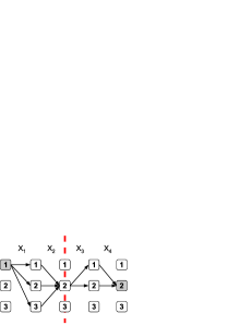
Figure 5: Layered graph for a Regular constraint.

6 Implementation

Our implementation of DDS extends Gecode, a C++ constraint programming library. In this section, we give an overview of relevant technical details of Gecode, and discuss the four main additions to Gecode that enable DDS: access to the constraint graph, decomposing global constraints, integrating Decompose into the search heuristic, and specialized search engines. The additions to Gecode comprise only 2500 lines (5%) of C++code and enable the use of DDS in any CSP modeled in Gecode. DDS will be available as part of the next release of Gecode.

6.1 Gecode

The Gecode library [11] is an open source constraint solver implemented in C++. It lends itself to a prototype implementation of DDS because of four facts:

1. Full source code enables changes to the available propagators.

2. The reflection capabilities allow access to the constraint graph.

3. Search is based on recomputation and copying, which significantly eases the implementation of specialized branchings and search engines.

4. It provides good performance, so that benchmarks give meaningful results.

6.2 Constraint graph

In most CP systems, the constraint graph is implicit in the data structures for variables and propagators. Gecode, e.g., maintains a list of propagators, and each propagator has access to the variables it depends on.

For DDS, a more explicit representation is needed that supports the computation of connected components. We can thus either maintain an additional, explicit constraint graph during propagation and search, or extract the graph from the implicit information each time we need it. For the prototype implementation, we chose the latter approach. We make use of Gecode’s reflection API, which allows to iterate over all propagators and their variables. Through reflection, we construct a graph using data structures from the boost graph library [6], which also provides the algorithm that computes connected components.

Assigned variables are independent of all other variables as discussed in Sec. 4. Therefore, they are reported as individual partial problems (connected components) but are ignored to avoid useless trivial decompositions without any effect. Instead these already solved single variable CSPs are added to an arbitrary partial problem that covers at least one unassigned variable. If the final number of such “non-solved” partial problems is at least two, a problem decomposition is initialised. This significantly speeds up the search process because only profitable decompositions are done.

6.3 Global constraint decomposition

As discussed in Sec. 5, it is absolutely essential for the success of DDS to consider constraint decompositions of global constraints when computing the connected components.

There are two possible implementation strategies for decomposing global constraints. A propagator can either detect decomposability during propagation and replace itself with several propagators on subsets of the variables. Or, alternatively, the constraint decompositions are only computed on demand when the constraint graph is required for connected component analysis. We implemented the latter option.

This again leaves two possible implementations. When the constraint graph is decomposed, one propagator (for a global constraint) may belong to two connected components. When search continues in the individual components, we can either use the propagator as it is in both components, or replace it by its decomposition. The latter option has the advantage that the smaller propagator may be more efficient (as it can ignore the variables outside its connected component). However, for simplicity, we implemented the former.

6.4 Decomposing branchings

Once we have identified connected components in the constraint graph, we have to create the partial problems that correspond to these components. In Gecode, we exploit the duality of choice and decomposition: both add branches to the search tree. The following observation leads to a simple and efficient implementation. If the heuristic is restricted such that it only selects variables inside one connected component, also propagation will only occur for variables of that component: For $\hat{\mathcal{X}}$ independent in $P$, ${\operatorname{propagate}(P)}_{|\hat{\mathcal{X}}}=\operatorname{propagate}({P}_{|\hat{\mathcal{X}}})$.

For our Gecode implementation, Decompose is thus realized as a branching. A branching in Gecode usually implements LeftChoice/RightChoice. For DDS, we extend it to also implement Decompose: If decomposition is possible, the branching limits further search to the variables in one connected component per branch. Otherwise, it just creates the usual choices according to the heuristic.

Branchings in Gecode are fully programmable. They have to support two operations: description and commit. description returns an abstract description of the possible branches while commit executes the branching according to a given description and alternative number.

A decomposing branching in Gecode is a wrapper around a standard variable-value branching. The actual work is done by description: it requests the constraint graph and performs the connected component analysis. If decomposition is possible, a special description is returned, representing the independent subsets $\hat{{\mathcal{X}}_{i}}\subset{\mathcal{X}}$. Otherwise, description is delegated to the embedded variable-value branching. Note that Gecode supports $n$-ary branchings, so decompositions do not have to be binary (as presented so far).

When commit is invoked with a variable-value description, the call is again delegated to the embedded branching. For a decomposition description, the branching’s list of variables is updated to $\hat{{\mathcal{X}}_{i}}$ for branch $i$, those still active in the selected component.

6.5 Decomposition search engines

As decomposition is performed by the branching, the search engines have to be specialized accordingly. We developed four search engines for DDS. A counting search engine computes the number of solutions of a given problem. A general-purpose search engine allows to incrementally search the whole tree and access all the partial solutions. Based on that we provide a search engine that enumerates all full solutions. A graphical search engine based on Gecode’s Gist (graphical interactive search tool) displays the search tree with special decomposition nodes, and allows to get an overview of where and how a particular problem can be decomposed. Figure 6 shows a screen shot of a partial search using DDS. Circular nodes with inner squares represent decompositions. All search engines accept cut-off parameters for the number of (full, not partial!) solutions to be explored.

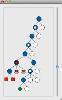
Figure 6: Gist, with decomposition nodes

7 Applications and Empirical Results

To illustrate possible use cases of DDS we applied it to two counting problems with global constraints. At first, the widely known graph coloring problem allows for a good and scalable illustration of the DDS effects due to the coherence of problem and constraint graph structure. It serves therefore as a model to investigate the impact of the problem structure on DDS in the presence of global constraints. Afterwards, we study the benefit of DDS on the real world problem of optimal protein structure prediction. This problem can be modelled using constraint programming [2] but necessitates the presence of global constraints covering the whole problem. Thus, the discussed constraint decomposition is an essential prerequisite to enable DDS.

Both applications show tremendous reductions in runtime and search tree size.

The applications were realized using our DDS implementation in Gecode. Only the search strategy was changed (DFS to DDS) – modeling, variable and value selection were kept the same for an appropriate comparison of the results. We chose maximal degree with minimal domain size as tie breaker as dynamic variable selection, which enforces decomposition and works well for DFS, too.

7.1 Graph coloring

Graph coloring is an important and hard problem with applications in scheduling, assignment of radio frequencies, and computer optimization [17, 23, 26]. A proper coloring assigns different colors to adjacent nodes. We want the chromatic polynomial for the chromatic number, i.e. the number of graph colorings with minimal colors. Graph coloring is a useful benchmark, because it gives us a scalable problem, so that we can apply DDS to instances of varying complexity.

The constraint model. For a given undirected graph $g$ and a number of colors $c$ we introduce one variable per node with the initial domains $0..(c-1)$. For each maximal clique of size $>2$, we post an All-different constraint on the corresponding variables. This maximizes the propagation necessary to solve these problems but still enables DDS as we discuss below. For all remaining edges we add binary inequality constraints.

The test sets. We generated the two test sets GC-30 and GC-50 of graphs with 30 and 50 nodes. For each size, random graphs were obtained by inserting an edge of the complete graph with a fixed uniform edge probability $P^{e}$. This was done using the Erdős-Rényi random graph generator GTgraph [12]. For each edge probability $P^{e}$ from 16 to 40 percent, 2000 graphs were generated and their colorings counted via DFS and DDS. To test highly degenerated problems (with many solutions) as well, we stopped after 1 million solutions.

Results. For the test sets, Tab. 1 compares the time consumption and search tree size by average ratios of DFS and DDS ($\frac{DFS}{DDS}$). A figure of 100 thus means that DDS is 100 times faster than DFS, or that the DFS search tree has 100 times as many nodes as the one for DDS. A dash means that most of the problems were not solved within a given time-out.

DFS/DDS:	Test set	16 %	18 %	20 %	22 %
rel. RT:	GC-30	411.2	197.7	75.74	34.6
	GC-50	242.7	151.8	34.23	16.5
ST size:	GC-30	680.3	344.4	142.0	74.48
	GC-50	646.1	383.8	94.28	47.26
DFS/DDS:	Test set	24 %	28 %	32 %	40 %
rel. RT:	GC-30	23.1	11.9	3.85	2.14
	GC-50	18.2	3.4	2.71	–
ST size:	GC-30	62.27	33.96	10.90	4.97
	GC-50	41.69	11.6	9.28	–

Table 1: Average ratios of DFS vs. DDS for various edge probabilities (RT = runtime, ST = search tree)

The presented runtime ratios show the high speedup for graphs with edge probabilities $P^{e}\leq 40$%. The distribution of speedup is exemplified in Fig. 7. The speedup corresponds to an even larger reduction of the search tree for DDS, which was only increased for 0.5% of all problems. Furthermore, sparse graphs yield a much higher runtime improvement than dense graphs, visualized by Fig. 8. The number of fails and propagations show no significant effect of DDS in contrast to runtime or search tree size.

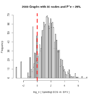
Figure 7: Histogram of logarithmic speedup for $P^{e}=28$ and 30 nodes (the dashed line marks equal runtime).

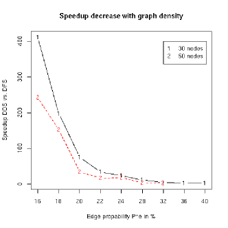
Figure 8: Avg. speedup decrease from 400 to 2 by graph density.

Still, the search tree reduction is not completely reflected in runtime speedup, which illustrates the computational overhead of DDS in the current prototypic implementation. Anyway, our data shows that DDS is well suited to improve solution counting even for dense graphs with $P^{e}$ about 40%. We expect even higher speedups and search-tree reductions if the solutions are counted completely, i.e. without the current upper bound of 1 million. Table 1 suggests that the speedup decreases with increasing number of nodes to color in the graph. With increasing number of nodes, the graph as well as the constraint graph grow quadratically.

The speedup is significantly lower than the reduction of the search tree. In part this can be ascribed to our implementation that rebuilds the constraint graph in each search step. A system that provides cheaper constraint graph access, e.g. by maintaining it incrementally, is expected to perform much better.

7.2 Optimal protein structure prediction

The prediction of optimal (minimal energy) structures of simplified lattice proteins is a hard (NP-complete) problem in bioinformatics. Here we focus on the HP-model introduced by Lau and Dill [13]. In this model, a protein chain is reduced to a sequence of monomers of equal size, whereby the 20 aminoacids are grouped into hydrophobic (H) or polar (P). A structure is a self-avoiding walk of the underlying lattice (e.g. square or cubic). A contact energy function is used to determine the energy of a structure. The energy table and an example is given in Fig. 9. The problem is to predict minimal energy structures for a given HP-sequence.

The number and quality of optimal structures has applications in the study of energy landscape properties, protein evolution and kinetics [9, 20, 25].

a) H P H -1 0 P 0 0	b)
c)

Figure 9: (a) Contact energy function (b) Example HP-structure with energy -2 (H-monomer: black, P-monomer: white, structure back bone: grey, HH-contact: dotted) (c) Compression of the solution space from 9 complete down to 3 by 3 partial structures.

The constraint model. In [2], the problem was successfully modeled as CSP and named Constraint-based Protein Structure Prediction (CPSP). Here, a variable is introduced for each sequence position and with lattice points as domains. The self-avoiding walk is modeled by a sequence of binary neighboring constraints (ensuring the connectivity of successive monomers) and a global All-different constraint for self-avoidingness. Supporting decomposition of the All-different propagator, see Sec. 5, is therefore essential for profiting from DDS.

CPSP uses a database of pre-calculated point sets, called H-cores, that represent possible optimal distributions of H-monomers. By that, the optimization problem is reduced to a satisfaction problem for a given H-core, if H-variables are restricted to these positions. For optimal H-cores, the solutions of the CSP are optimal structures. Thus, for counting all optimal structures, one iterates through the optimal cores.

The test sets. We generated two test sets, PS-48 and PS-64, with uniformly distributed random HP-sequences of length 48 and 64. For the generation we used the free available CPSP implementation [7]. With only minimal modifications (new branching) we use the existing CSP model with DDS.

PS-48 contains 6350 HP-sequences and for each up to 1 million optimal structures in the cubic lattice were predicted. For the 2630 HP-sequences in PS-64 up to 2 million structures have been predicted in the cubic lattice, due to the increasing degeneracy in sequence length.

Results. The average ratio results are given in Tab. 2. There, the enormous search tree reduction with an average factor of 11 and 25 respectively is shown. The reduction using DDS compared to DFS leads to much less propagations (3- to 5-fold). This and the slightly less fails result in a runtime speedup of 3-/4-fold using the same variable selection heuristics for both search strategies. Here, the immense possibilities of DDS even without advanced constraint-graph specific heuristics are demonstrated. This also shows the rising advantage of DDS over DFS for increasing problem sizes (with higher solution numbers).

DFS / DDS
 runtime  ST size  fails  propagations PS-48 2.98 11.30 1.40 3.27 PS-64 4.23 25.33 1.76 5.43

Table 2: Average ratios for CPSP using DFS vs. DDS (ST = search tree)

8 Discussion

The paper introduces decomposition during search (DDS), an integration of And/Or search with propagation-based constraint solvers. DDS dynamically decomposes CSPs, avoiding much of the redundant work of standard tree search when exploring huge search spaces, e.g. of $\#P$-hard counting problems.

We discuss the interaction of DDS with such vital and essential features as global constraints and dynamic variable ordering. The techniques presented here have been implemented for Gecode.

The empirical evaluation on graph coloring and protein structure prediction shows the huge potential of DDS in terms of search tree size reduction and already high true runtime speedup. The speedup proves that DDS can be implemented competitively, and with a reasonable overhead. We expect even higher speedups by improving the constraint graph representation and its incremental maintenance, which is a current area of development. However, one experience from our experiments is that it is highly problem-specific whether the constraint graph allows for decomposition. We partly explain this by pointing out that some constraints (e.g. linear (in-)equations) inherently hinder decomposition.

We envision promising future research in the following directions. First, providing efficient access to the constraint graph. Second, the development of specifically tailored heuristics for DDS focusing on dynamic variable selection or domain splitting. Such heuristics should employ information about the constraint graph, to decompose the problem as often as possible and in a well-balanced way. Decomposition-directed heuristics might however counteract problem specific heuristics. Balancing such heuristics is a further research direction.

Finally, solving optimization problems using And/Or branch-and-bound (BAB) search [15] seems an obvious extension. However, our first experiments using a prototypical DDS extension of BAB show much smaller benefits than for counting (similar to the results in [15, 16]).

Acknowledgements. We thank Christian Schulte and Mikael Lagerkvist for fruitful discussions about the architecture and the paper, and the reviewers of earlier versions of this paper for constructive comments. Martin Mann is supported by the EU project EMBIO (EC contract number 012835). Sebastian Will is partially supported by the EU Network of Excellence REWERSE (project number 506779).

References

- [1] O. Angelsmark and P. Jonsson. Improved algorithms for counting solutions in constraint satisfaction problems. In Proc. of 9th CP, pages 81–95, 2003.
- [2] R. Backofen and S. Will. A constraint-based approach to fast and exact structure prediction in 3D protein models. Constraints, 11(1):5–30, 2006.
- [3] R. J. Bayardo Jr. and J. D. Pehoushek. Counting models using connected components. In Proc. of the 7th National Conference on AI, pages 157–162, 2000.
- [4] C. Bessiere, E. Hebrard, B. Hnich, Z. Kiziltan, C.-G. Quimper, and T. Walsh. Reformulating global constraints: the SLIDE and REGULAR constraints. In Proc. of SARA-2007, pages 80–92, 2007.
- [5] A. Biere and C. Sinz. Decomposing SAT problems into connected components. Satisfiability, Boolean Modeling and Computation, 2:191–198, 2006.
- [6] Boost graph library, 2007. Available as an open-source library from www.boost.org.
- [7] CPSP: Tools for constraint-based protein structure prediction, 2006. Available as an open-source library from www.bioinf.uni-freiburg.de/sw/cpsp.
- [8] R. Dechter and R. Mateescu. The impact of AND/OR search spaces on constraint satisfaction and counting. In Proc. of 10th CP, pages 731–736, 2004.
- [9] C. Flamm, I. L. Hofacker, P. F. Stadler, and M. T. Wolfinger. Barrier trees of degenerate landscapes. Z.Phys.Chem, 216:155–173, 2002.
- [10] E. C. Freuder and M. J. Quinn. Taking advantage of stable sets of variables in constraint satisfaction problems. In Proc. of 9th IJCAI, pages 1076–1078, 1985.
- [11] Gecode: Generic constraint development environment, 2007. Available as an open-source library from www.gecode.org.
- [12] GTgraph: A suite of synthetic graph generators, 2006. Available as an open-source library from www-static.cc.gatech.edu/~kamesh/GTgraph.
- [13] K. F. Lau and K. A. Dill. A lattice statistical mechanics model of the conformational and sequence spaces of proteins. ACS, 22:3986 – 3997, 1989.
- [14] W. Li and P. van Beek. Guiding real-world SAT solving with dynamic hypergraph separator decomposition. In Proc. of 16th IEEE ICTAI, pages 542–548, 2004.
- [15] R. Marinescu and R. Dechter. AND/OR branch-and-bound for graphical models. In Proc. of 19th IJCAI, pages 224–229, 2005.
- [16] R. Marinescu and R. Dechter. Dynamic orderings for and/or branch-and-bound search in graphical models. In ECAI, pages 138–142, 2006.
- [17] L. Narayanan and S. M. Shende. Static frequency assignment in cellular networks. Algorithmica, 29(3):396–409, 2001.
- [18] G. Pesant. A regular language membership constraint for finite sequences of variables. In Proc. of 10th CP, pages 482–495, 2004.
- [19] G. Pesant. Counting solutions of CSPs: A structural approach. In Proc. of 19th IJCAI, pages 260–265, 2005.
- [20] A. Renner and E. Bornberg-Bauer. Exploring the fitness landscapes of lattice proteins. In 2nd. Pacif. Symp. Biocomp. Singapore, 1997.
- [21] D. Roth. On the hardness of approximate reasoning. Artif. Intelligence, 82(1-2):273–302, 1996.
- [22] J.-C. Régin. A filtering algorithm for constraints of difference in CSPs. In Proc. of 12th National Conference on AI, pages 362–367, 1994.
- [23] Y.-T. Tsai, Y.-L. Lin, and F. R. Hsu. The on-line first-fit algorithm for radio frequency assignment problems. Inf. Process. Lett., 84(4):195–199, 2002.
- [24] L. G. Valiant. The complexity of computing the permanent. Theoretical Computer Science, 8(2):189–201, 1979.
- [25] M. Wolfinger, S. Will, I. Hofacker, R. Backofen, and P. Stadler. Exploring the lower part of discrete polymer model energy landscapes. EPL, 74:725–732, 2006.
- [26] H.-G. Yeh and X. Zhu. Resource-sharing system scheduling and circular chromatic number. Theor. Comput. Sci., 332(1-3):447–460, 2005.