Inflation and Quintessence: Theoretical Approach of Cosmological Reconstruction

Abstract:

In the first part of this paper, we outline the construction of an inflationary cosmology in the framework where inflation is described by a universally evolving scalar field $\phi$ with potential $V(\phi)$. By considering a generic situation that inflaton attains a nearly constant velocity, during inflation, $m_{\lower 2.0pt\hbox{$\scriptstyle P$}}^{-1}|d\phi/dN|\equiv\alpha+\beta\exp(\beta N)$ (where $N\equiv\ln a$ is the e-folding time), we reconstruct a scalar potential and find the conditions that have to satisfied by the (reconstructed) potential to be consistent with the WMAP inflationary data. The consistency of our model with WMAP result (such as $n_{\lower 2.0pt\hbox{$\scriptstyle s$}}=0.951^{+0.015}_{-0.019}$ and $r<0.3$) would require $0.16<\alpha<0.26$ and $\beta<0$. The running of spectral index, $\widetilde{\alpha}\equiv dn_{\lower 2.0pt\hbox{$\scriptstyle s$}}/d\ln k$, is found to be small for a wide range of $\alpha$.

In the second part of this paper, we introduce a novel approach of constructing dark energy within the context of the standard scalar-tensor theory. The assumption that a scalar field might roll with a nearly constant velocity, during inflation, can also be applied to quintessence or dark energy models. For the minimally coupled quintessence, $\alpha_{\lower 2.0pt\hbox{$\scriptstyle Q$}}\equiv dA(Q)/d(\kappa Q)=0$ (where $A(Q)$ is the standard matter-quintessence coupling), the dark energy equation of state in the range $-1\leq w_{\lower 2.0pt\hbox{$\scriptstyle\rm DE$}}<-0.82$ can be obtained for $0\leq\alpha<0.63$. For $\alpha<0.1$, the model allows for only modest evolution of dark energy density with redshift. We also show, under certain conditions, that the $\alpha_{\lower 2.0pt\hbox{$\scriptstyle Q$}}>0$ solution decreases the dark energy equation of state $w_{\lower 2.0pt\hbox{$\scriptstyle Q$}}$ with decreasing redshift as compared to the $\alpha_{\lower 2.0pt\hbox{$\scriptstyle Q$}}=0$ solution. This effect can be opposite in the $\alpha_{\lower 2.0pt\hbox{$\scriptstyle Q$}}<0$ case. The effect of the matter-quintessence coupling can be significant only if $|\alpha_{\lower 2.0pt\hbox{$\scriptstyle Q$}}|\gtrsim 0.1$, while a small coupling $|\alpha_{\lower 2.0pt\hbox{$\scriptstyle Q$}}|<0.1$ will have almost no effect on cosmological parameters, including $\Omega_{\lower 2.0pt\hbox{$\scriptstyle Q$}}$, $w_{\lower 2.0pt\hbox{$\scriptstyle Q$}}$ and $H(z)$. The best fit value of $\alpha_{\lower 2.0pt\hbox{$\scriptstyle Q$}}$ in our model is found to be $\alpha_{\lower 2.0pt\hbox{$\scriptstyle Q$}}\simeq 0.06$, but it may contain significant numerical errors, viz $\alpha_{\lower 2.0pt\hbox{$\scriptstyle Q$}}=0.06\pm 0.35$, which thereby implies the consistency of our model with general relativity (for which $\alpha_{\lower 2.0pt\hbox{$\scriptstyle Q$}}=0$) at $1\sigma$ level.

1 Introduction and Overview

It is true and remarkable that our understanding of the physical universe has deepened profoundly in the last few decades through thoughts, experiments and observations. Along with significant advancements in observational cosmology [1, 2, 3], Einstein’s general relativity has been established as a successful classical theory of gravitational interactions, from scales of millimeters through to kiloparsecs ($1$ pc$=3.27$ light years). It has also been learned that at very short distance scales large quantum fluctuations make gravity very strongly interacting, implying that general relativity cannot be used to probe spacetime (geometry) for distances close to Planck’s length, $l_{P}\sim 10^{-33}~{}{\rm cm}$. In addition to this difficulty, three striking facts about nature’s clues suggest that we are missing a few important parts of the picture, notably the extreme weakness of gravity relative to the other forces, the huge size and flatness of the observable universe, and the late time cosmic acceleration.

Much is not understood: what is the nature of the mysterious smooth dark energy and the clumped non-baryonic dark-matter, which respectively form $73\%$ and $22\%$ of the mass-energy in the universe. That means, we do not see and really understand yet about $95\%$ of the total matter density of the universe. To understand the need for dark energy, or a mysterious force propelling the universe, and dark matter, one has to look at the different constituents of the universe, their properties and observational evidences (for reviews, see, e.g. [4, 5, 6, 7]). The current standard model of cosmology somehow combines the original hot big bang model and the early universe inflation, by virtue of the existence of a fundamental scalar field, called inflaton. The standard model of cosmology is, however, not completely satisfactory and it appears to have some gaps. If the universe is currently accelerating (on largest scales), what recent observations seem to indicate, then we need in the fabric of the cosmos a self-repulsive dark energy component, or a cosmological constant term, which had almost no role in the early universe, or need to modify Einstein’s theory of gravity on largest scales in order to explain this acceleration.

When in 1917 Einstein proposed the field equations for general relativity

$$R_{\mu\nu}-\frac{1}{2}\,Rg_{\mu\nu}+\Lambda g_{\mu\nu}=8\pi G_{N}\,T_{\mu\nu},$$ (1)

he had the choice of adding an extra term proportional to the metric $g_{\mu\nu}$ either on the left-hand or right-hand side of eq. (1). This extra term, so-called the cosmological constant $\Lambda$, is not fixed by the structure of the theory. One also finds no good reason to set it to zero either, unless the underlying theory is purely supersymmetric. Adding the term $\Lambda g_{\mu\nu}$ on the left hand side of his famous equation, Einstein used to tune the constant $\Lambda$ in such a way that he would get a non-expanding solution. Einstein later dismissed the cosmological constant as his “greatest blunder”, when Hubble found a clear indication for an (ever) expanding universe. Today this constant is mainly written on the right hand side of the Einstein equations but still with a positive sign, which therefore acts as an extra repulsive force (or dark energy) in cosmological (time-dependent) backgrounds.

Before presenting further thoughts on the nature of this puzzling form of energy, it is logical to recapitulate the independent pieces of evidence for its existence. The key measurements, leading to the result of DE density fraction being $\Omega_{\rm DE}\simeq 0.7$ have been made, rather unexpectedly, in 1998 by two independent groups (Supernova Cosmology Project and High-z Supernova Search Team)  [1]. These observations revealed, for the first time, that the universe is not only expanding now but its expansion is speeding up for the last $5-6$ billion years, i.e. since when the redshift $z$ dropped below $0.85$.

Evidence for the existence of dark energy also comes from observations of the Cosmic Microwave Background (CMB) for which the most recent ones have been obtained by NASA’s Wilkinson Microwave Anisotropy Probe (WMAP) [3]. As first observed in 1992 by the COBE satellite [8] and afterwards by several other ground-and balloon-based experiments, the nearly perfect black body spectrum of the CMB has little temperature fluctuations of the order $\delta T/T\sim\frac{18\mu K}{2.725K}\sim 10^{-5}$. The angular size of these fluctuations encodes the density and velocity fluctuations at the surface of last scattering, with redshift $z\simeq 1100$. This corresponds to the cosmological epoch when the presently observed CMB photons first decoupled from matter. By plotting the squared of amplitude of CMB temperature fluctuations against their wavelengths (or multipoles in an equivalent Fourier power spectrum), there can be allocated several peaks at different angular sizes. The position of the first peak is often viewed as an indicator for the spatial curvature of the universe, which reveals that the present universe is nearly flat and homogeneous on large cosmological scales ($>100~{}{\rm Mpc}$), meaning that $\Omega_{tot}\approx 1$ with high accuracy. However, when assuming a flat universe only containing pressureless dust (including DM) and assuming the current Hubble parameter to be $h=0.72\pm 0.08$ with $H_{0}=100{\rm h\,km}\,{\rm sec}^{-1}\,{\rm Mpc}^{-1}$ (in agreement with observations of the Hubble Space Telescope Key project [9]), it is figured out that $t_{0}=9\pm 1Gyrs$. This result, simply following from Einstein’s general relativity, implies that a flat universe without the cosmological constant term may suffer from a serious age problem. Introducing DE in the form of a constant $\Lambda$, with $\Omega_{\Lambda,0}\simeq 0.73$, somehow resolves the problem, giving $t_{0}\simeq 13.8~{}{\rm Gyrs}$ with $h=0.72$.

When accepting the existence of DE, naturally the question arises, what it really is. Since the late $1960^{\prime}s$ when it was realized that [10] the zero point vacuum fluctuations in quantum field theories are Lorentz invariant, it has been attempted to associate this (quantum) vacuum energy with the present value of $\Lambda$ but without much success. Even when placing a cutoff at some reasonable energy scale, this quantum vacuum energy is still several orders of magnitude larger than the mysterious dark energy today, $\rho_{\Lambda}\sim 5\times 10^{-47}~{}{\rm GeV^{4}}$ or $\rho_{\Lambda}\sim 10^{-123}$ in Planck units (for reviews, see, e.g. [11, 12]). Apparently, $\rho_{\lower 2.0pt\hbox{$\scriptstyle\Lambda$}}^{1/4}$ is fifteen orders of magnitude smaller than the electroweak scale, $m_{\lower 2.0pt\hbox{$\scriptstyle EW$}}\sim 10^{12}~{}{\rm eV}$. No theoretical model, not even the most sophisticated, such as supersymmetry or string theory, is able to explain the presence of a small positive $\Lambda$.

Another hurdle in understanding the nature of dark energy is that only a very small window in the magnitude of the cosmological constant allows the universe to develop as it obviously has. It is still a mystery why $\Omega_{\Lambda}$ has the value it has today. It could have been several magnitudes of order larger or smaller than the matter density today, instead of $\Omega_{\Lambda}\simeq 3\Omega_{\lower 2.0pt\hbox{$\scriptstyle\rm m$}}$. This is known as cosmological coincidence problem.

At present the most common view is that dark energy is presumably constant and has a constant equation of state, $w_{\lower 2.0pt\hbox{$\scriptstyle DE$}}=-1$. But there remains the possibility that the cosmological constant (or the gravitational vacuum energy) is fundamentally variable. In a more realistic picture, at least, from field theoretic viewpoints, dark energy should be dynamical in nature [13]. This is the case, for instance, with all time dependent solutions arising out of evolving scalar fields, with an accelerated expansion coming from modified gravity models, holographic dark energy, and the likes.

Interestingly enough, the recent observations (WMAP+SDSS [3]) only demand that $-1.04<w_{\lower 2.0pt\hbox{$\scriptstyle DE$}}<-0.82$. In view of this wide range for the present value of dark energy equation of state (EoS), it is certainly worth constructing an explicit model cosmology, where dark energy arises because of a dynamically evolving scalar field, and see what other consequences would arise from such a modification of Einstein’s general relativity.

2 Constructing Inflationary Cosmology

A complete model of the universe should perhaps feature a period of inflation in a distant past, leading to a generation of density (or scalar) perturbations via quantum fluctuations. This expectation has now received considerable observational support from measurements of anisotropies in the CMB as detected by WMAP and other experiments.

In the simplest class of inflationary models, inflation is described by a single scalar (or an inflaton) field $\phi$, with some potential $V(\phi)$. The corresponding action is

$$S=\int d^{4}{x}\sqrt{-g}\left(\frac{R}{2\kappa^{2}}-\frac{1}{2}(\partial\phi)^{2}-V(\phi)\right),$$ (2)

where $\kappa\equiv m_{P}^{-1}=\left(8\,\pi\,G_{N}\right)^{1/2}$ is the inverse Planck mass, with $G_{N}$ being Newton’s constant, $\sqrt{-g}=\det g_{\mu\nu}$ is the determinant of the metric tensor.

Constructing concrete models of inflation and matching them to the CMB and large scale structure (LSS) experiments has become one of the major pursuits in cosmology. Most earlier studies regarding the form of an inflationary potential relied on a prior choice of the potential $V(\phi)$, or on slow-roll approximations in the calculation of power spectra and their relation to the mass of the field $\phi$ during inflation (see [14] for a review). The latter approach can at best produce the tail of an inflationary potential, but not its full shape [15]. Indeed, recent studies show that the type or variety of scalar potential allowed by array of WMAP inflationary data is still large [16]. Although, in order to understand the dynamics of inflation, the idea of utilizing one or the other form of the scalar field potential (motivated by physics beyond the standard model or even by theories of higher dimensional gravity, such as, string theory) is not bad at all, there might exist a more elegant way of confronting the WMAP inflationary data with a theoretical model.

In this paper we present a different and robust approach to tackle this problem: we do not make a specific choice for $V(\phi)$, rather we make a simple ansatz for the scalar field $\phi$ and then construct an inflationary potential, using the symmetry of Einstein’s field equations. Our approach would be novel in the sense that it provides a unique shape (and slope) to the scalar (or inflaton) potential. The model also makes falsifiable predictions. The basic ideas and some of the results were presented in a recent paper [17].

For simplicity, we consider a spatially flat Friedmann-Robertson-Walker spacetime. The evolution of the field $\phi$ is then described by the equation (see, e.g. [18])

$$\dot{\phi}=m_{\lower 2.0pt\hbox{$\scriptstyle P$}}(-2\dot{H})^{1/2}=-2m_{\lower 2.0pt\hbox{$\scriptstyle P$}}^{2}\frac{d}{d\phi}H(\phi)$$ (3)

and the evolution of the scalar potential $V(\phi)$ is governed by

$$\frac{V(\phi)}{m_{\lower 2.0pt\hbox{$\scriptstyle P$}}^{2}}=3H^{2}(\phi)+\dot{\phi}\frac{d}{d\phi}H(\phi)=3H^{2}(\phi)-2m_{\lower 2.0pt\hbox{$\scriptstyle P$}}^{2}\left[\frac{d}{d\phi}H(\phi)\right]^{2},$$ (4)

where $H(\phi(t))\equiv\dot{a}/a$ is the Hubble parameter and $a(t)$ is the FRW scale factor, and the dot denotes a derivative with respect to the cosmic time $t$.

Let us first briefly discuss how the model that we are going to construct could satisfy inflationary constraints from the WMAP and other experiments. First, note that the term

$$2m_{\lower 2.0pt\hbox{$\scriptstyle P$}}^{2}\left[\frac{d}{d\phi}H(\phi)\right]^{2}$$

is usually non-negligible (as compared to $3H^{2}(\phi)$) at the onset of inflation. This would be the case, for instance, if the mass of the inflaton field, $m_{\lower 2.0pt\hbox{$\scriptstyle\phi$}}\equiv\left(d^{2}V(\phi)/d\phi^{2}\right)^{1/2}$, is large enough initially, $m_{\lower 2.0pt\hbox{$\scriptstyle\phi$}}\sim m_{\lower 2.0pt\hbox{$\scriptstyle P$}}$. Once the field $\phi$ rolls satisfying $|\ddot{\phi}|\ll 3H|\dot{\phi}|$, or equivalently, $\Delta\phi\propto\ln[a(t)]$, the scalar potential is well approximated by an exponential term:

$$V(\phi)\sim 3m_{\lower 2.0pt\hbox{$\scriptstyle P$}}^{2}H^{2}(\phi)\sim\frac{H_{\lower 2.0pt\hbox{$\scriptstyle 0$}}^{2}}{2}(6-{\phi^{\prime}}^{2})\,{\rm e}^{2\kappa\phi^{\prime}}\,{\rm e}^{\kappa^{2}\phi^{\prime}\phi}\sim\frac{H_{\lower 2.0pt\hbox{$\scriptstyle 0$}}^{2}}{2}(6-\alpha^{2}){\rm e}^{2\alpha}{\rm e}^{\alpha\kappa\phi},$$ (5)

where $\kappa\phi^{\prime}\equiv\alpha$ is the slope of the potential, during a slow-roll regime. The condition $\kappa\dot{\phi}<\sqrt{6}H$ holds in general, so $V(\phi)>0$. Inflation occurs as long as the condition

$$\frac{\ddot{a}}{a}=H^{2}(\phi)-2m_{\lower 2.0pt\hbox{$\scriptstyle P$}}^{2}\left(\frac{dH(\phi)}{d\phi}\right)^{2}>0$$

holds, meaning that $V(\phi)>\dot{\phi}^{2}$. But, after a sufficient number of e-folds of expansion, inflation has to end. This is possible when the quantity $(m_{\lower 2.0pt\hbox{$\scriptstyle P$}}/H(\phi))(dH(\phi)/d\phi)$ becomes comparable to (or even larger than) unity. Recent results from WMAP [3] indicate that the spectral index of the scalar perturbations is consistent with almost flat one, $n_{\lower 2.0pt\hbox{$\scriptstyle s$}}=0.958^{+0.015}_{-0.019}$. To a good approximation, $1-n_{\lower 2.0pt\hbox{$\scriptstyle s$}}\simeq\alpha^{2}$, implying that $\alpha<0.25$. This simple picture has obvious and intuitive appeal, which can be realized through an explicit construction.

To illustrate the construction, we make the following ansatz

$$\frac{\phi}{m_{\lower 2.0pt\hbox{$\scriptstyle P$}}}\equiv{\rm const}-\alpha\ln\left(\frac{a}{a_{\lower 2.0pt\hbox{$\scriptstyle i$}}}\right)-\left(\frac{a}{a_{\lower 2.0pt\hbox{$\scriptstyle i$}}}\right)^{\beta},$$ (6)

where $a_{\lower 2.0pt\hbox{$\scriptstyle i$}}$ is the initial value of the scale factor before inflation, and $\alpha$ and $\beta$ are free parameters for now. We take $\beta<0$, so that after few number of e-folds, since $a\gg a_{\lower 2.0pt\hbox{$\scriptstyle i$}}$, the inflaton $\phi$ naturally satisfies $\frac{\phi^{\prime}}{m_{\lower 2.0pt\hbox{$\scriptstyle P$}}}=\frac{1}{m_{\lower 2.0pt\hbox{$\scriptstyle P$}}}\frac{d\phi}{d\ln a}\simeq-\alpha$. One may think that the above choice for $\phi$ is ad hoc and/or no more motivated than a particular choice of $V(\phi)$, but it is not exactly! Indeed (6) is the property of an inflaton field in many well motivated inflationary models that satisfy slow roll conditions, after a few e-folds of inflation. It can also be compared to a generic solution for a dilaton (or modulus field), i.e. $\phi(t)\sim\phi_{\lower 2.0pt\hbox{$\scriptstyle 0$}}+\alpha_{\lower 2.0pt\hbox{$\scriptstyle 0$}}\ln t+\alpha_{\lower 2.0pt\hbox{$\scriptstyle 1$}}/t^{\gamma}$ (where $\gamma>0$), in four-dimensional superstring models (see, e.g. [19, 18]). Additionally, the ansatz (6) allows us to construct an explicit inflationary model, providing an appropriate shape (and slope) to the scalar field potential.

The evolution of $\phi$ as given in eq. (6) is provided by the Hubble parameter

$$H(\phi)=H_{\lower 2.0pt\hbox{$\scriptstyle 0$}}\exp\left[{-\frac{\alpha^{2}}{2}N(\phi)}-\alpha\,e^{-\beta N(\phi)}-\frac{\beta}{4}\,e^{-2\beta N(\phi)}\right],$$ (7)

where $N(\phi)\equiv\ln(a/a_{\lower 2.0pt\hbox{$\scriptstyle i$}})$, $a\equiv a(\phi(t))$ and $H_{\lower 2.0pt\hbox{$\scriptstyle 0$}}$ is an integration constant. We can easily evaluate the following two inflationary variables

$$\epsilon_{\lower 2.0pt\hbox{$\scriptstyle H$}}(\phi) = {2m_{\lower 2.0pt\hbox{$\scriptstyle P$}}^{2}}\left(\frac{1}{H}\frac{dH(\phi)}{d\phi}\right)^{2}=\frac{1}{2}\left(\alpha+\beta\,e^{\beta N(\phi)}\right)^{2},$$ (8)

$$\eta_{\lower 2.0pt\hbox{$\scriptstyle H$}}(\phi) = 2m_{\lower 2.0pt\hbox{$\scriptstyle P$}}^{2}\frac{1}{H(\phi)}\left(\frac{d^{2}H(\phi)}{d\phi^{2}}\right)=\epsilon_{\lower 2.0pt\hbox{$\scriptstyle H$}}-\frac{\beta^{2}}{\beta+\alpha\,{\rm e}^{-\beta N(\phi)}}$$ (9)

(which are first-order in slow roll approximations). The magnitude of these quantities must be much smaller than unity, during inflation, in order to get a sufficient number of e-folds of expansion, like ${\cal N}_{e}\equiv\ln(a_{\lower 2.0pt\hbox{$\scriptstyle f$}}/a_{\lower 2.0pt\hbox{$\scriptstyle i$}})\gtrsim 50$. More precisely, we require $|\epsilon_{\lower 2.0pt\hbox{$\scriptstyle H$}}|\ll 1$, $|\eta_{\lower 2.0pt\hbox{$\scriptstyle H$}}|<1$, except near to the exit from inflation where $\epsilon_{\lower 2.0pt\hbox{$\scriptstyle H$}}\gtrsim 1$. One may actually demand that $0\leq\epsilon_{\lower 2.0pt\hbox{$\scriptstyle H$}}\leq 3$, so that the scalar field potential

$$V(\phi)=m_{\lower 2.0pt\hbox{$\scriptstyle P$}}^{2}H^{2}(\phi)\left(3-\epsilon_{\lower 2.0pt\hbox{$\scriptstyle H$}}\right)$$ (10)

is non-negative. A typical shape of this potential is depicted in Fig. 1. The magnitude of $H_{\lower 2.0pt\hbox{$\scriptstyle 0$}}$ (cf eq. (7)) can be fixed using the amplitude of density perturbations observed at the COBE experiments, using the normalization [20]:

$$(dV/d\phi)^{-1}V^{3/2}/(\sqrt{75}\pi m_{\rm Pl}^{3})\simeq 1.92\times 10^{-5}.$$

Typically, with $\alpha\sim 0.2$ and ${\cal N}_{e}\equiv\ln(a_{\lower 2.0pt\hbox{$\scriptstyle f$}}/a_{\lower 2.0pt\hbox{$\scriptstyle i$}})\sim 55$, we find (assuming that $\beta<0$)

$$H_{\lower 2.0pt\hbox{$\scriptstyle 0$}}\sim 7.42\times 10^{-5}\,m_{\lower 2.0pt\hbox{$\scriptstyle P$}}.$$ (11)

This is a perfectly reasonable value, which also characterizes the average energy scale of inflation in most inflationary models.

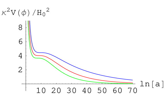
Figure 1: The shape of the potential, for some representative values of $\alpha=0.2,~{}0.3,~{}0.4$ (top to bottom), $\beta=-\,0.2$ and $N(\phi)\equiv\ln a+c$. We have taken $c=-10$.

As long as the parameter $\epsilon_{\lower 2.0pt\hbox{$\scriptstyle H$}}(\phi)$ is slowly varying, the scalar curvature perturbation can be shown to be [21]

$$P_{\lower 2.0pt\hbox{$\scriptstyle\cal R$}}^{1/2}(k)=2^{\nu-3/2}\frac{\Gamma(\nu)}{\Gamma(3/2)}(1-\epsilon_{\lower 2.0pt\hbox{$\scriptstyle H$}})^{\nu-1/2}\left(\frac{H^{2}}{2\pi|\dot{\phi}|}\right)_{\lower 2.0pt\hbox{$\scriptstyle aH=k$}},$$ (12)

where $\nu=3/2+1/(p-1)$ and $a\propto t^{p}$. The scalar spectral index $n_{\lower 2.0pt\hbox{$\scriptstyle s$}}$ for $P_{\lower 2.0pt\hbox{$\scriptstyle\cal R$}}$ is defined by

$$n_{\lower 2.0pt\hbox{$\scriptstyle s$}}(k)\equiv 1+\frac{d\ln P_{\lower 2.0pt\hbox{$\scriptstyle\cal R$}}}{d\ln k}.$$ (13)

The fluctuation power spectrum is in general a function of wave number $k$, and is evaluated when a given comoving mode crosses outside the (cosmological) horizon during inflation: $k=aH=a_{\lower 2.0pt\hbox{$\scriptstyle e$}}H(\phi)e^{-\Delta N}$ is, by definition, a scale matching condition and $a_{\lower 2.0pt\hbox{$\scriptstyle e$}}$ is the value of the scale factor at the end of inflation. Instead of specifying the fluctuation amplitude directly as a function of $k$, it is convenient to specify it as a function of the number of $e$-folds ${\cal N}_{e}$ of expansion between the epoch when the horizon scale modes left the horizon and the end of inflation. To leading order in slow roll parameters, $n_{s}$ is given by [14]

$$n_{\lower 2.0pt\hbox{$\scriptstyle s$}}-1=2\eta_{\lower 2.0pt\hbox{$\scriptstyle H$}}-4\epsilon_{\lower 2.0pt\hbox{$\scriptstyle H$}}=-\frac{\alpha^{3}+3\alpha^{2}\mu+3\alpha\mu^{2}+2\beta\mu+\mu^{3}}{\alpha+\mu},$$ (14)

where $\mu\equiv\beta{\rm e}^{\beta{\cal N}_{e}}$. In the conventional case that $\beta=0$, which corresponds to a scenario where inflation is driven by a simple exponential potential, $V(\phi)\propto{\rm e}^{\alpha(\phi/m_{\lower 2.0pt\hbox{$\scriptstyle P$}})}$, we obtain a well known result that $1-n_{\lower 2.0pt\hbox{$\scriptstyle s$}}\simeq\alpha^{2}$. Here we shall assume that ${\cal N}_{e}\geq 47$ and $\beta<0$.

Let us also define the slope or running of the spectral index $n_{\lower 2.0pt\hbox{$\scriptstyle s$}}$, which is given by

$$\widetilde{\alpha}\equiv\frac{dn_{\lower 2.0pt\hbox{$\scriptstyle s$}}}{d\ln k}=\frac{dn_{s}}{dN}\frac{dN}{d\phi}\frac{d\phi}{d\ln k}$$ (15)

(tilde is introduced here to avoid confusion with the exponent parameter $\alpha$ introduced in eq. (6)), where $\phi$ and $k$ are related by

$$\frac{d\phi}{d\ln k}=-m_{\lower 2.0pt\hbox{$\scriptstyle P$}}\frac{\sqrt{2\epsilon_{\lower 2.0pt\hbox{$\scriptstyle H$}}(\phi)}}{(1-\epsilon_{\lower 2.0pt\hbox{$\scriptstyle H$}}(\phi))},$$ (16)

while $N$ and $\phi$ are related by

$$m_{\lower 2.0pt\hbox{$\scriptstyle P$}}\frac{dN}{d\phi}=-\frac{1}{\sqrt{2\epsilon_{\lower 2.0pt\hbox{$\scriptstyle H$}}(\phi)}}.$$ (17)

These relations hold independent of our ansatz (6).

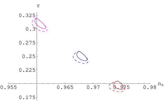
Figure 2: The tensor-to-scalar ratio $r\simeq 16\epsilon_{\lower 2.0pt\hbox{$\scriptstyle H$}}$ vs the scalar spectral index $n_{\lower 2.0pt\hbox{$\scriptstyle s$}}$ with $\alpha=0.2,0.18$ and $0.16$ (top to bottom) and $\beta=(-0.5,0)$. The solid (dotted) lines are for ${\cal N}_{e}=60$ (${\cal N}_{e}=47$).

The WMAP bound on the tensor-to-scalar ratio, $r\simeq 16\epsilon_{\lower 2.0pt\hbox{$\scriptstyle H$}}<0.3$ ($95\%$ confidence level), implies $\epsilon_{\lower 2.0pt\hbox{$\scriptstyle H$}}<0.0187$. This bound is satisfied for

$$\alpha\lesssim 0.1936\quad{\rm and}\quad n_{\lower 2.0pt\hbox{$\scriptstyle s$}}\gtrsim 0.9624.$$ (18)

The spectral index obtained in this way is within the range indicated by three year WMAP results [3]

$$n_{\lower 2.0pt\hbox{$\scriptstyle s$}}=0.958^{+0.015}_{-0.019}.$$ (19)

Of course, one may directly use the above bound for $n_{\lower 2.0pt\hbox{$\scriptstyle s$}}$ and find the corresponding bound on $r$. Again by demanding that ${\cal N}_{e}\gtrsim 50$ and $\beta\lesssim-0.2$, we find

$$\alpha=0.2213^{-0.0360}_{+0.0394},\qquad r=0.3918^{-0.1200}_{+0.1520}.$$ (20)

The smaller is the value of $\alpha$, the smaller will be the tensor-to-scalar ratio (see Fig. 2), allowing only a small running of spectral index. For instance, if $|\alpha|\lesssim 0.1$ and $\beta\lesssim-0.2$, then we find

$$n_{\lower 2.0pt\hbox{$\scriptstyle s$}}\gtrsim 0.98,\qquad r<0.08.$$ (21)

The WMAP data requires a spectral index that is significantly less than the Harrison-Zel’dovich-Peebles scale-invariant spectrum ($n_{\lower 2.0pt\hbox{$\scriptstyle s$}}=1$, $r=0$). Thus, given that $\beta<0$, consistency of our model (with WMAP result) seems to require $0.16<\alpha<0.26$.

         

Figure 3: Contour plots for $n_{\lower 2.0pt\hbox{$\scriptstyle s$}}=0.95$ with ${\cal N}_{e}=50$ (left plot) and ${\cal N}_{e}=60$ (right plot).

It is also significant to note that, for $\alpha\ll|\beta|$, there exists a small window in the parameter space where

$$n_{\lower 2.0pt\hbox{$\scriptstyle s$}}\simeq 0.95,\qquad r\sim{\cal O}(10^{-3}-10^{-6}),$$

in which case, however, the slope parameters $\alpha$ and $\beta$ must be finely tuned. In Fig. 3 we show the contour plots with ${\cal N}_{e}=50$ and ${\cal N}_{e}=60$, representing such a case. In fact, in the case $|\alpha|<0.05$, the gravity waves (or tensor modes) are almost nonexistent. On the right plot in Fig. 4 we show the running of spectral index $\widetilde{\alpha}$, which is always very small in the parameter range $0.1<\alpha<1$ and $\beta<0$.

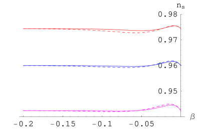
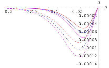
Figure 4: The scalar spectral index $n_{\lower 2.0pt\hbox{$\scriptstyle s$}}$ (left plot) and its running $\widetilde{\alpha}$ with respect to $\beta$ and $\alpha=0.16,0.20$ and $0.24$ (top to bottom). The solid (dotted) lines are for ${\cal N}_{e}=60$ (${\cal N}_{e}=47$). The running of $n_{s}$ could be large only if $|\alpha|\lesssim|\beta|$; for example, $\widetilde{\alpha}\simeq-0.004$ for $\alpha\simeq 0.01$ and $\beta\simeq-0.05$.

In a model with more than one scalar field, the dependency of inflationary variables like $n_{\lower 2.0pt\hbox{$\scriptstyle s$}}$ and $r$ on the slope parameters $\alpha$ and $\beta$ could be more complicated than the simplest explanation provided above. Nonetheless, our approach has great significance as it generically leads to a spectrum of primordial scalar fluctuations that is slightly red-tilted ($n_{\lower 2.0pt\hbox{$\scriptstyle s$}}\lesssim 1$) and hence compatible with WMAP inflationary data.

3 Constructing Quintessence Cosmology

It is reasonable to assume that a late time acceleration of the universe is driven by the same mechanism usually exploited to give early universe inflation, where the potential energy of a scalar field dominates its kinetic term. To this end, let us assume that the current expansion of the universe can be described by the action

$$S=S_{\rm grav}+S_{m}=\int d^{4}{x}\sqrt{-g}\left(\frac{R}{2\kappa^{2}}-\frac{1}{2}\,(\nabla{Q})^{2}-V({Q})\right)+S_{m},$$ (22)

where $Q$ is a fundamental scalar (or dark energy) field, $V(Q)$ is its potential, $S_{\rm grav}$ is the gravitational part of the action, $S_{m}$ is the matter action describing the dynamics of ordinary fields (matter and radiation) and $\nabla$ represents a four-dimensional covariant derivative. The matter part of the action (22) can be written as

$$S_{m}=\int d^{4}{x}\,{\cal L}(\psi_{\lower 2.0pt\hbox{$\scriptstyle m$}},A^{2}({Q})g_{\mu\nu})\equiv\int d^{4}{x}\sqrt{-g}\,A^{4}({Q})\,\sum_{i}\rho_{i},$$ (23)

where $\psi_{m}$ represents collectively the matter degrees of freedom and radiation. In the above definition of the matter Lagrangian, the implicit assumption is that matter couples to $\tilde{g}_{\mu\nu}\equiv A({Q})^{2}g_{\mu\nu}$, rather than the Einstein metric $g_{\mu\nu}$ alone. This assumption then results in a non-minimal coupling between the scalar field ${Q}$ and matter components ($\rho_{i}$). The matter-scalar coupling $A(Q)$ may be understood as a natural modification of Einstein’s GR which can be motivated by, for instance, scalar-tensor theory. For further discussions on theoretical motivations of this coupling, see, for example,[23, 24, 25, 26].

The coupling $A({Q})$ actually generates a new term, namely

$$-\frac{2}{\sqrt{-g}}\,\frac{\delta{\cal L}_{m}^{(i)}}{\delta{Q}}\equiv\frac{dA({Q})}{d{Q}}\,T_{\mu\,(i)}^{\,\mu},$$ (24)

in the scalar wave equation for $Q$. This expression also implies that radiation does not couple to the scalar field ${Q}$ since its trace of the energy-momentum tensor equals zero. As we will show the coupling $\frac{dA({Q})}{d{Q}}$ introduces several qualitatively new cosmological features.

As is well known, the cosmological constant case (or more generally Einstein gravity with a cosmological term) arises as a special limit of the present model, for which

$$\frac{\partial Q}{\partial t}=0$$ (25)

and hence $V({Q})={\rm const}\equiv\Lambda$ and $A(Q)={\rm const}$. The model then reduces to the $\Lambda$CDM cosmology, given that dark matter is characterized by non-relativistic particles alone, $w_{\lower 2.0pt\hbox{$\scriptstyle m$}}=0$. The cosmological term $\Lambda$, which is governed by the equation

$${m_{\lower 2.0pt\hbox{$\scriptstyle P$}}^{2}}\,G^{\mu}_{\nu}=2\Lambda\delta^{\mu}_{\nu}+T^{\mu}_{\nu},$$ (26)

can clearly act as a source of gravitational repulsion or putative dark energy.

All the discussions so far have been made without making any particular choice of metric. Thus the nature of $V(Q)$ acting as a repulsive force is rather general. For a more detailed treatment, it is necessary to evaluate the equations generated by variation of the total action $S=S_{\lower 2.0pt\hbox{$\scriptstyle\rm grav$}}+S_{\lower 2.0pt\hbox{$\scriptstyle m$}}$. Therefore a particular choice of a metric has to be made. We make rather standard choice of a spatially flat FRW metric:

$$ds^{2}=-dt^{2}+a\left(t\right)^{2}\,d{\bf x}^{2},$$ (27)

where $a(t)$ is the scale factor of a FRW universe. This choice of the line element is well motivated by the observational fact that the universe is spatially flat on largest scales, which is consistent with the concept of inflation, discussed in the previous section. Of course, this choice of metric may lead to systematic errors in the calculation, as the universe actually is not homogenous at smaller (or galactic) scales, as pointed out, for example, in [22], which is ignored in this simplified assumption.

In the minimal coupling case, $A({Q})\equiv 1$, it is easy to see that

$$\rho_{\lower 2.0pt\hbox{$\scriptstyle i$}}\propto\left[a(t)\right]^{-3\,\left(1+w_{i}\right)},$$ (28)

where $w_{\lower 2.0pt\hbox{$\scriptstyle i$}}\equiv p_{i}/\rho_{i}$. In the non-minimal coupling case the modified scale factor $\widehat{a}$ is given by $\widehat{a}=a(t)\,A(Q)$. As a consequence, different equation of state parameters (cf eq. (24)) would cause different energy densities to evolve differently with changing scale factor:

$$\rho_{\lower 2.0pt\hbox{$\scriptstyle i$}}\propto(a(t)\,A(Q))^{-3\,\left(1+w_{\lower 2.0pt\hbox{$\scriptstyle i$}}\right)}.$$ (29)

This implies that $\rho_{m}\propto(a(t)A({Q}))^{-3}$ and $\rho_{r}\propto\left(a(t)A({Q})\right)^{-4}$, respectively, for ordinary matter and radiation. It also shows that radiation never directly couples to the scalar field, even with $A({Q})$ being an arbitrary function of ${Q}$. As explained in [17], the coupling $A({Q})$ can be relevant, especially, in a background where $\rho_{\lower 2.0pt\hbox{$\scriptstyle m$}}$ is much larger than $\rho_{\lower 2.0pt\hbox{$\scriptstyle\rm crit$}}$ (where $\rho_{\lower 2.0pt\hbox{$\scriptstyle\rm crit$}}\equiv 3H_{\lower 2.0pt\hbox{$\scriptstyle 0$}}^{2}/8\pi G$), e.g., a galactic environment.

3.1 Basic Equations

Taking a variation of the action (22) with respect to $g^{\mu\nu}$ and then evaluating the $tt$ and $xx$ components of Einstein’s equation leads to the following two equations (cf eq. (A.1)):

$$-\frac{3}{\kappa^{2}}\,H^{2}+\frac{1}{2}\,\dot{{Q}}^{2}+V\left({Q}\right)+A^{4}\left({Q}\right)\,\sum_{i}\rho_{\lower 2.0pt\hbox{$\scriptstyle i$}}=0$$ (30)

$$\frac{1}{\kappa^{2}}\,\left(2\,\dot{H}+3\,H^{2}\right)+\frac{1}{2}\,\dot{{Q}}^{2}-V\left({Q}\right)+A^{4}\left({Q}\right)\,\sum_{i}\left(w_{\lower 2.0pt\hbox{$\scriptstyle i$}}\,\rho_{\lower 2.0pt\hbox{$\scriptstyle i$}}\right)=0$$ (31)

A variation with respect to the scalar field ${Q}$, while considering an explicit matter-scalar coupling, yields the following equation of motion for $Q$ (cf eq. (A.2)):

$$\ddot{{Q}}+3\,H\,\dot{{Q}}+\frac{dV\left({Q}\right)}{d{Q}}-A^{3}\,\frac{dA\left({Q}\right)}{d{Q}}\,\sum_{i}\left(1-3\,w_{\lower 2.0pt\hbox{$\scriptstyle i$}}\right)\,\rho_{\lower 2.0pt\hbox{$\scriptstyle i$}}=0,$$ (32)

the so-called the Klein-Gordon equation for ${Q}$. It shows that the scalar field ${Q}$ couples to the trace of the energy-momentum tensor $g^{\mu\nu}T_{\mu\nu}$ satisfying

$$-\nabla^{2}{Q}=\ddot{{Q}}+3H\dot{{Q}}=-\frac{d\,V({Q})}{d\,{Q}}-A^{3}\,\frac{dA\left({Q}\right)}{d{Q}}\,T_{\lower 2.0pt\hbox{$\scriptstyle\mu$}}^{\mu}.$$ (33)

There is dissension about the sign of the coupling term between the scalar field and matter in above equation in the way that it might be $+A^{3}\,\frac{dA\left({Q}\right)}{d{Q}}\,T_{\lower 2.0pt\hbox{$\scriptstyle\mu$}}^{\mu}$ instead of $-A^{3}\,\frac{dA\left({Q}\right)}{d{Q}}\,T_{\lower 2.0pt\hbox{$\scriptstyle\mu$}}^{\mu}$. In this paper, the negative sign, as written in eq. (32), will be used.

The above set of equations can be supplemented by a fourth equation, arising from the equation of motion for a perfect barotropic fluid

$$\left(a\,A\right)\,\frac{d\rho_{\lower 2.0pt\hbox{$\scriptstyle i$}}}{d\left(a\,A\right)}=-\rho_{\lower 2.0pt\hbox{$\scriptstyle i$}}\,3\,\left(1+w_{\lower 2.0pt\hbox{$\scriptstyle i$}}\right).$$ (34)

This finally leads to (cf eq. (A.7), see also [27])

$$\dot{\rho_{\lower 2.0pt\hbox{$\scriptstyle i$}}}+3H\left(1+w_{\lower 2.0pt\hbox{$\scriptstyle i$}}\right)\rho_{\lower 2.0pt\hbox{$\scriptstyle i$}}=\frac{\dot{{Q}}}{A}\frac{dA\left({Q}\right)}{d{Q}}\,\left(1-3\,w_{\lower 2.0pt\hbox{$\scriptstyle i$}}\right)\,\rho_{\lower 2.0pt\hbox{$\scriptstyle i$}}.$$ (35)

Out of the four equations (30)-(32) and (35), only three are independent, meaning the conservation equation of the perfect fluid (35) can be derived without the assumption (34) but only by combining (30)-(32). General covariance requires the conservation of the total energy density, $\rho_{\lower 2.0pt\hbox{$\scriptstyle\rm tot$}}=\rho_{\lower 2.0pt\hbox{$\scriptstyle Q$}}+\sum\rho_{\lower 2.0pt\hbox{$\scriptstyle i$}}$, which is obviously the case in our model (see also the appendix in [28]).

Next we make the following substitutions:

$$\epsilon\equiv\frac{\dot{H}}{H^{2}}=\frac{H^{\prime}}{H},\quad\Omega_{\lower 2.0pt\hbox{$\scriptstyle i$}}\equiv\frac{\kappa^{2}\,A^{4}\,\rho_{\lower 2.0pt\hbox{$\scriptstyle i$}}}{3\,H^{2}},\quad\Omega_{{Q}}\equiv\frac{\kappa^{2}\,\left(\frac{1}{2}\,\dot{{Q}}^{2}+V\left({Q}\right)\right)}{3\,H^{2}}\equiv\frac{\kappa^{2}\,\rho_{{Q}}}{3\,H^{2}},$$ (36)

and

$$w_{\lower 2.0pt\hbox{$\scriptstyle Q$}}\equiv\frac{\frac{1}{2}\,\dot{{Q}}^{2}-V\left({Q}\right)}{\frac{1}{2}\,\dot{{Q}}^{2}+V\left({Q}\right)}\equiv\frac{p_{{Q}}}{\rho_{{Q}}}.$$ (37)

These substitutions and further simplifications lead to the set of four equations:

$$\sum_{i}\Omega_{\lower 2.0pt\hbox{$\scriptstyle i$}}+\Omega_{{Q}}=1$$ (38)

$$2\,\epsilon+3\,\left(1+w_{\lower 2.0pt\hbox{$\scriptstyle Q$}}\right)\,\Omega_{{Q}}+3\,\sum_{i}\left(1+w_{\lower 2.0pt\hbox{$\scriptstyle i$}}\right)\,\Omega_{\lower 2.0pt\hbox{$\scriptstyle i$}}=0$$ (39)

$$\Omega_{{Q}}^{\prime}+2\,\epsilon\,\Omega_{{Q}}+3\,\Omega_{{Q}}\,\left(1+w_{\lower 2.0pt\hbox{$\scriptstyle Q$}}\right)+{Q}^{\prime}\,\alpha_{\lower 2.0pt\hbox{$\scriptstyle Q$}}\,\sum_{i}\left(\eta_{i}\,\Omega_{\lower 2.0pt\hbox{$\scriptstyle i$}}\right)=0$$ (40)

$$\sum_{i}\Omega_{\lower 2.0pt\hbox{$\scriptstyle i$}}^{\prime}+2\,\epsilon\,\sum_{i}\Omega_{\lower 2.0pt\hbox{$\scriptstyle i$}}+3\,\sum_{i}\left(\Omega_{\lower 2.0pt\hbox{$\scriptstyle i$}}\,\left(1+w_{\lower 2.0pt\hbox{$\scriptstyle i$}}\right)\right)-{Q}^{\prime}\,\alpha_{\lower 2.0pt\hbox{$\scriptstyle Q$}}\,\sum_{i}\left(\eta_{i}\,\Omega_{\lower 2.0pt\hbox{$\scriptstyle i$}}\right)=0,$$ (41)

where, as above, the prime denotes a derivative with respect to e-folding time $N\equiv\ln[a(t)]+{\rm const}$, $Q^{\prime}\equiv\dot{Q}/H$, $\eta_{\lower 2.0pt\hbox{$\scriptstyle i$}}\equiv 1-3w_{\lower 2.0pt\hbox{$\scriptstyle i$}}$ and $\alpha_{\lower 2.0pt\hbox{$\scriptstyle Q$}}\equiv\frac{d\ln\left[A(Q)\right]}{d{\kappa Q}}$. In the above we have used the relation

$$\frac{\partial}{\partial N}=\frac{1}{H}\,\frac{\partial}{\partial t}.$$ (42)

Equations (38)-(41) represent the most general case of an evolving universe based on the general action (22). Equation (38) is simply the Friedmann constraint for the assumed flat universe. Changing the sign of the coupling $\alpha_{\lower 2.0pt\hbox{$\scriptstyle Q$}}$ to the trace of the energy-momentum tensor $T^{\mu}_{\mu}$ in eq. (33) would cause a change of sign from $+{Q}^{\prime}\,\alpha_{\lower 2.0pt\hbox{$\scriptstyle Q$}}\,\sum_{i}\left(\eta_{i}\,\Omega_{\lower 2.0pt\hbox{$\scriptstyle i$}}\right)$ to $-{Q}^{\prime}\,\alpha_{\lower 2.0pt\hbox{$\scriptstyle Q$}}\,\sum_{i}\left(\eta_{i}\,\Omega_{\lower 2.0pt\hbox{$\scriptstyle i$}}\right)$ in eq. (40). Adding eqs. (40) and (41), we find

$$\Omega_{{Q}}^{\prime}+2\,\epsilon\,\Omega_{{Q}}+3\,\Omega_{{Q}}\,\left(1+w_{\lower 2.0pt\hbox{$\scriptstyle Q$}}\right)+\sum_{i}\Omega_{\lower 2.0pt\hbox{$\scriptstyle i$}}^{\prime}+2\,\epsilon\,\sum_{i}\Omega_{\lower 2.0pt\hbox{$\scriptstyle i$}}+3\,\sum_{i}\left(\Omega_{\lower 2.0pt\hbox{$\scriptstyle i$}}\,\left(1+w_{\lower 2.0pt\hbox{$\scriptstyle i$}}\right)\right)=0,$$ (43)

which can be interpreted as a global energy conservation equation. Thus, for not violating this principle of energy conservation (43), a sign change in (40) automatically implies a change in (41) as well.

When having a particular solution of the equations (38)-(41), it is of great interest to study how the corresponding potential looks like and how it affects the cosmic evolution of our universe. From the last expression in eq. (36), we find

$$V\left({Q}\right)\equiv H^{2}\,\left(\frac{3\,\Omega_{{Q}}}{\kappa^{2}}-\frac{1}{2}\,\left({Q}^{\prime}\right)^{2}\right),$$ (44)

which will be used later. Of course, in the case of a minimal coupling ($A({Q})\equiv 1$), $\alpha_{\lower 2.0pt\hbox{$\scriptstyle Q$}}$ vanishes, reducing the number of degrees of freedom in the system of equations (38)-(41) by one, which then makes the system easier to handle. Anyhow in both cases ($\alpha_{\lower 2.0pt\hbox{$\scriptstyle Q$}}=0$ and $\alpha_{\lower 2.0pt\hbox{$\scriptstyle Q$}}\neq 0$) it is not possible to find an analytical solution of this system without making some additional assumptions as there are more degrees of freedom than independent equations. In fact, the number of degrees of freedom depends on the number of matter components included in the analysis.

As the first check for compatibility of the model, it is useful to consider some simplified solution of the equations (35)-(41), by expressing all matter fields as one component, $w_{\lower 2.0pt\hbox{$\scriptstyle i$}}\equiv w_{\lower 2.0pt\hbox{$\scriptstyle m$}}$. By applying eq. (42) to eq. (35), and after a simple integration, we get

$$\rho_{\lower 2.0pt\hbox{$\scriptstyle m$}}=\rho_{\lower 2.0pt\hbox{$\scriptstyle m$}}^{(0)}\,e^{-3\ln{a}}\,\exp\left[\int\left({Q}^{\,\prime}\alpha_{\lower 2.0pt\hbox{$\scriptstyle Q$}}\,\left(3\,w_{\lower 2.0pt\hbox{$\scriptstyle m$}}-1\right)+3\,w_{\lower 2.0pt\hbox{$\scriptstyle m$}}\right)d\ln{a}\right],$$ (45)

with $\rho_{\lower 2.0pt\hbox{$\scriptstyle m$}}^{(0)}$ being an arbitrary constant. The coupling $\alpha_{\lower 2.0pt\hbox{$\scriptstyle Q$}}$ may be constrained by observations perhaps only in the combination $Q^{\,\prime}\alpha_{\lower 2.0pt\hbox{$\scriptstyle Q$}}$. One can study the effect of this coupling on both CMB temperature anisotropies and evolution of linear matter perturbations, as in [29]. In the minimal coupling case, one has

$$\rho_{\lower 2.0pt\hbox{$\scriptstyle m$}}\propto a^{-3(1+w_{\lower 2.0pt\hbox{$\scriptstyle m$}})}.$$ (46)

This is exactly the behaviour one would expect from general relativity. Equation (46) yields $\rho_{\lower 2.0pt\hbox{$\scriptstyle m$}}\propto a^{-3}$ in a universe containing only ordinary matter (or dust), while for radiation $\rho_{r}\propto a^{-4}$. Transposing eq. (39) leads to a general expression for the equation of state of the DE component which can generally be written as

$$w_{\lower 2.0pt\hbox{$\scriptstyle Q$}}=-\frac{2\,\epsilon+3\,\sum_{i}\left(1+w_{\lower 2.0pt\hbox{$\scriptstyle i$}}\right)\,\Omega_{\lower 2.0pt\hbox{$\scriptstyle i$}}+3\,\Omega_{{Q}}}{3\,\Omega_{{Q}}},$$ (47)

where all possible forms of matter are included, e.g. pressureless dust ($w_{\rm m}=0$), radiation ($w_{\rm r}=1/3$), stiff matter ($w_{\rm sm}=1$), domain walls ($w_{\rm dw}=-2/3$), etc.

For further analysis, it is useful to introduce the so called effective equation of state parameter $w_{\lower 2.0pt\hbox{$\scriptstyle\rm eff$}}$, which is defined by

$$w_{\lower 2.0pt\hbox{$\scriptstyle\rm eff$}}\equiv\frac{p_{\rm tot}}{\rho_{\rm tot}},\quad p_{\rm tot}\equiv p_{{Q}}+\widetilde{p}_{\lower 2.0pt\hbox{$\scriptstyle i$}},\quad\rho_{\rm tot}\equiv\rho_{{Q}}+\widetilde{\rho}_{\lower 2.0pt\hbox{$\scriptstyle i$}},$$ (48)

whereas $p_{{Q}}$ and $\rho_{{Q}}$ are as defined in eq. (37), and $\widetilde{p}_{\lower 2.0pt\hbox{$\scriptstyle i$}}\equiv A^{4}(Q)p_{\lower 2.0pt\hbox{$\scriptstyle i$}}$, $\widetilde{\rho}_{\lower 2.0pt\hbox{$\scriptstyle i$}}\equiv A^{4}(Q)\rho_{\lower 2.0pt\hbox{$\scriptstyle i$}}$. The meaning of $w_{\lower 2.0pt\hbox{$\scriptstyle\rm eff$}}$ is somehow that of a mean equation of state of all matter-energy components, including the dark energy component $\rho_{\lower 2.0pt\hbox{$\scriptstyle Q$}}$. From eq. (39), together with eqs.(36)-(37), we find that the total pressure is given by

$$p_{\lower 2.0pt\hbox{$\scriptstyle\rm tot$}}=\frac{3\,H^{2}}{\kappa^{2}}\,\left(-\frac{2\,\epsilon}{3}-\Omega_{{Q}}-\sum_{i}\Omega_{\lower 2.0pt\hbox{$\scriptstyle i$}}\right).$$ (49)

Combining this expression for $p_{\lower 2.0pt\hbox{$\scriptstyle\rm tot$}}$ with the expression of total energy density $\rho_{\lower 2.0pt\hbox{$\scriptstyle tot$}}$, as defined by (48), and using again the substitutions (36)-(37), we get

$$w_{\lower 2.0pt\hbox{$\scriptstyle\rm eff$}}=-1-\frac{2\,\epsilon}{3}.$$ (50)

This expression is valid even in the most general non-minimal coupling case. Similarly, we can define the deceleration parameter $q$ as

$$q\equiv-\frac{\ddot{a}}{a\,H^{2}}=-1-\epsilon,$$ (51)

showing that the name “deceleration parameter” makes sense in such a way that $q>0$ for a decelerated expansion ($\ddot{a}<0$), while $q<0$ for an accelerating expansion ($\ddot{a}>0$).

As explained in the Introduction, one reason for considering a universe containing a nonzero DE component, either in the form of a cosmological constant $\Lambda$ or a dynamically evolving scalar field ${Q}$, is the recently observed accelerated expansion of the universe by the Supernova Cosmology Project and the High-redshift Supernova Search team  [1]. Thus we find it useful to study the solution of equations (38) to (41), which yields an accelerated expansion in a general context of nontrivial matter-scalar coupling.

Indeed, independent of any assumption or specific composition of the universe, simply the condition $w_{\lower 2.0pt\hbox{$\scriptstyle\rm eff$}}<-1/3$ at some stage of cosmic evolution yields an accelerated solution. It should be noted at this stage, that no such general connection can be established between the DE equation of state parameter $w_{\lower 2.0pt\hbox{$\scriptstyle Q$}}$ having a specific value (even like $w_{\lower 2.0pt\hbox{$\scriptstyle Q$}}=-1$) and the universe being in an accelerating phase.

In the notations used in this paper, both the non-baryonic (cold) dark matter and ordinary matter (pressureless dust) are combined in one matter constituent $\Omega_{\lower 2.0pt\hbox{$\scriptstyle\rm m$}}$. As $w_{\lower 2.0pt\hbox{$\scriptscriptstyle DM$}}\approx 0$ is a rather good approximation for the equation of state of cold dark matter (since it is non-relativistic) this combination seems to be reasonable. This assumption as regards the composition of the universe today implies that its only constituents are cold dark matter, ordinary matter, radiation and DE. Putting this composition ($\Omega_{\lower 2.0pt\hbox{$\scriptstyle\rm m$}}\cong 0.27$, $\Omega_{{Q}}\cong 0.73$ and $\Omega_{\lower 2.0pt\hbox{$\scriptstyle\rm r$}}\cong 10^{-4}$) of today’s universe into the very general expression of the DE equation of state parameter $w_{\lower 2.0pt\hbox{$\scriptstyle Q$}}$ (cf eq. (47)) and using again $w_{\rm m}=0$ and $w_{\lower 2.0pt\hbox{$\scriptstyle Q$}}\simeq-1$, the value $\epsilon=-0.4$ is obtained. This implies that for $w_{\lower 2.0pt\hbox{$\scriptstyle Q$}}$ at least being close to $-1$ the universe is in an accelerating phase today, which is what is observed.

The general considerations so far seem to be consistent with observations. As observations seem to indicate a value for $w_{\lower 2.0pt\hbox{$\scriptstyle Q$}}$ close to $-1$, the possibility of a dark energy component simply being a cosmological constant cannot be ruled out. But it is also important to realize that the effects of a slowly rolling scalar field would be almost indistinguishable from that of a pure cosmological constant if $\kappa Q^{\,\prime}\equiv m_{\lower 2.0pt\hbox{$\scriptstyle P$}}^{-1}(\dot{Q}/H)\lesssim 0.1$ at present. Evidence for $w_{\lower 2.0pt\hbox{$\scriptstyle Q$}}\sim-1$ could actually imply that the field $Q$ is rolling only with a tiny velocity at present. This point should be more clear from the discussion below.

All the examinations so far have been in a rather general way without imposing any additional assumptions. For sure that is not really satisfying, as one might be interested in an analytic solution of the system of equations (38) to (41). As mentioned above this is not possible without further input because of the number of degrees of freedom exceeding the number of independent equations. In the next two subsections two different analytic solutions will be presented making some simple additional assumptions. According to the present constitution of the universe being $\Omega_{\lower 2.0pt\hbox{$\scriptstyle m$}}\simeq 0.27$ and $\Omega_{\lower 2.0pt\hbox{$\scriptstyle Q$}}\simeq 0.73$, it is reasonable to neglect the radiation component at least for redshift $z\lesssim{\cal O}(10)$. Therefore the model universe assumed in the next two sections is thought to only consist of cold dark matter and ordinary matter combined in one component with a common equation of state $w_{\rm m}=0$ and a DE component represented by the scalar field ${Q}$ with a variable EoS $w_{\lower 2.0pt\hbox{$\scriptstyle Q$}}$.

The system of equations (38)-(41) can then be expressed in the form:

$$\Omega_{\lower 2.0pt\hbox{$\scriptstyle\rm m$}}+\Omega_{{Q}} = 1$$ (52)

$$2\,\epsilon+3\,\left(1+w_{\lower 2.0pt\hbox{$\scriptstyle Q$}}\right)\,\Omega_{{Q}}+3\,\Omega_{\lower 2.0pt\hbox{$\scriptstyle\rm m$}} = 0$$ (53)

$$\Omega_{{Q}}^{\prime}+2\,\epsilon\,\Omega_{{Q}}+3\,\Omega_{{Q}}\,\left(1+w_{\lower 2.0pt\hbox{$\scriptstyle Q$}}\right)+{Q}^{\prime}\,\alpha_{\lower 2.0pt\hbox{$\scriptstyle Q$}}\,\Omega_{\lower 2.0pt\hbox{$\scriptstyle\rm m$}} = 0$$ (54)

$$\Omega_{\lower 2.0pt\hbox{$\scriptstyle\rm m$}}^{\prime}+2\,\epsilon\,\Omega_{\lower 2.0pt\hbox{$\scriptstyle\rm m$}}+3\,\Omega_{\lower 2.0pt\hbox{$\scriptstyle\rm m$}}-{Q}^{\prime}\,\alpha_{\lower 2.0pt\hbox{$\scriptstyle Q$}}\,\Omega_{\lower 2.0pt\hbox{$\scriptstyle\rm m$}} = 0.$$ (55)

The number of free parameters in this system is five ($\Omega_{\lower 2.0pt\hbox{$\scriptstyle\rm m$}}$, $\Omega_{{Q}}$, $w_{\lower 2.0pt\hbox{$\scriptstyle Q$}}$, $\epsilon$ and $\alpha_{\lower 2.0pt\hbox{$\scriptstyle Q$}}$), meaning two additional assumptions have to be made to find an analytic solution. To proceed further, we make the following assumption:

$${Q}={Q}_{0}+m_{\lower 2.0pt\hbox{$\scriptstyle P$}}\,{\alpha}\,\ln[a(t)]\equiv{Q}_{0}+m_{\lower 2.0pt\hbox{$\scriptstyle P$}}{\alpha}\,\left(N+{\rm const}\right),$$ (56)

where $\alpha$ is a constant which needs to be fixed by observations. This relation actually represents a generic situation that the field ${Q}$ is rolling with a constant velocity, $Q^{\,\prime}={\rm const}$ . In the minimal coupling case this is enough, while in the non-minimal case ($\alpha_{\lower 2.0pt\hbox{$\scriptstyle Q$}}\neq 0$) one more assumption is required, which will be discussed below.

Simply transposing (37) and utilizing the relation between $\frac{\partial}{\partial t}$ and $\frac{\partial}{\partial N}$, as given by (42), yields the following useful relation

$$w_{\lower 2.0pt\hbox{$\scriptstyle Q$}}=\frac{\kappa^{2}\,{{Q}^{\prime}}^{2}-3\,\Omega_{{Q}}}{3\,\Omega_{{Q}}}\equiv\frac{\alpha^{2}-3\,\Omega_{{Q}}}{3\,\Omega_{{Q}}}.$$ (57)

Supplementing equations (52)-(55) with this equation is an elegant way of imposing an additional constraint into the model.

3.2 Uncoupled Quintessence

In the $A(Q)=1$ case, the system of equations (52)-(55), supplemented by eq. (56), can now be solved analytically. The explicit solution is given by

$$\Omega_{{Q}} = 1-\frac{\lambda}{c_{\lower 2.0pt\hbox{$\scriptstyle 1$}}\lambda\,\exp\left[\lambda N\right]+3}$$ (58)

$$w_{\lower 2.0pt\hbox{$\scriptstyle Q$}} = \frac{-\,c_{\lower 2.0pt\hbox{$\scriptstyle 1$}}\lambda^{2}}{3\alpha^{2}\exp\left[-\lambda N\right]+3\lambda c_{\lower 2.0pt\hbox{$\scriptstyle 1$}}}$$ (59)

$$\epsilon = \frac{-c_{\lower 2.0pt\hbox{$\scriptstyle 1$}}\,\alpha^{2}\,\lambda-9\,\exp\left[-\lambda N\right]}{2\,c_{\lower 2.0pt\hbox{$\scriptstyle 1$}}\,\lambda+6\,\exp\left[-\lambda N\right]},$$ (60)

where $N\equiv N(Q)=\ln[a(Q(t))]$ and we have made the substitution

$$\lambda\equiv 3-\alpha^{2}.$$ (61)

Using eqs. (50) and (51) we also evaluate

$$q = \frac{3\,\exp\left[-\lambda N\right]-c_{\lower 2.0pt\hbox{$\scriptstyle 1$}}\,\left(6-5\,\alpha^{2}+\alpha^{4}\right)}{6\,\exp\left[-\lambda N\right]+2\,c_{\lower 2.0pt\hbox{$\scriptstyle 1$}}\,\lambda},$$ (62)

$$w_{\lower 2.0pt\hbox{$\scriptstyle\rm eff$}} = \frac{-\,c_{\lower 2.0pt\hbox{$\scriptstyle 1$}}\,\lambda^{2}}{9\,\exp\left[-\lambda N\right]+3\,c_{\lower 2.0pt\hbox{$\scriptstyle 1$}}\lambda}.$$ (63)

This general solution contains three free parameters ($N$, $\alpha$ and $c_{\lower 2.0pt\hbox{$\scriptstyle 1$}}$). To keep the solution as general as possible it is useful to just fix one free parameter in terms of the other two. The integration constant $c_{\lower 2.0pt\hbox{$\scriptstyle 1$}}$ can be fixed in terms of the field velocity $\alpha$ by using the observational input $\Omega_{\lower 2.0pt\hbox{$\scriptstyle m0$}}=0.27$ at present. The e-folding time $N$ in relation to the cosmic time $t$ is only defined up to an arbitrary constant, so it needs to be normalised in some way. For simplicity, this will be done by taking $N=0$ at present. Thus, the condition $\Omega_{\lower 2.0pt\hbox{$\scriptstyle\rm m$}}[N=0,\alpha,c_{\lower 2.0pt\hbox{$\scriptstyle 1$}}]\equiv\Omega_{\lower 2.0pt\hbox{$\scriptstyle m0$}}$ yields

$$c_{\lower 2.0pt\hbox{$\scriptstyle 1$}}=\frac{3-\alpha^{2}-3\Omega_{\lower 2.0pt\hbox{$\scriptstyle m0$}}}{(3-\alpha^{2})\Omega_{\lower 2.0pt\hbox{$\scriptstyle m0$}}},$$ (64)

which now makes it possible to express eqs. (58)-(60) just in terms of the two free parameters $N$ and $\alpha$. For further analysis it is useful to parameterize the solution in terms of redshift $z$. By utilising the dependence of the redshift on the scale factor $a(t)$, it is easy to obtain the relation between $N$ and $z$:

$$z+1=\frac{\lambda_{obs}}{\lambda_{em}}=\frac{a_{0}}{a\left(t\right)},\quad\exp[N]=\frac{a(t)}{a_{0}}=\frac{1}{1+z}.$$ (65)

Here $t$ is the time when light was emitted, that is observed now. Thus choosing $a_{0}$ to be the present scale factor automatically implies the normalization $N=0$ at $z=0$. From eqs. (58)-(60), one can clearly see that the solution is symmetric in $\alpha$ as only even powers of $\alpha$ occur. Thus, without loss of generality, in the further analysis only positive $\alpha$ will be considered. For the value of $c_{\lower 2.0pt\hbox{$\scriptstyle 1$}}$ satisfying (64), and $\Omega_{\lower 2.0pt\hbox{$\scriptstyle m0$}}\simeq 0.27$, it is easy to see that $c_{\lower 2.0pt\hbox{$\scriptstyle 1$}}=0$ for $\alpha^{2}=2.19$, implying that $\alpha_{\lower 2.0pt\hbox{$\scriptstyle\rm crit$}}=1.48$. This value of $\alpha$ has some significance, when looking at the evolution of $w_{\lower 2.0pt\hbox{$\scriptstyle Q$}}$ for different values of $\alpha$.

         

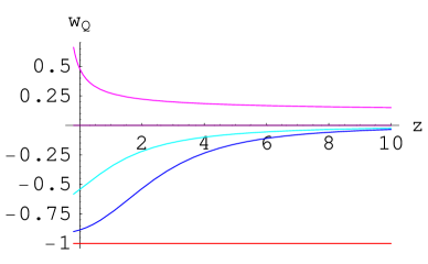
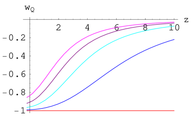
Figure 5: $w_{\lower 2.0pt\hbox{$\scriptstyle Q$}}$ with respect to redshift $z$ (left plot) for $\alpha=0$, $0.5$, $1.0$, $1.48$, $1.8$, and (right plot) $\alpha=0$, $0.15$, $0.3$, $0.45$, $0.6$ (bottom to top).

From the left plot in Fig. 5 it is easily seen that $\alpha=1.48$ yields $w_{\lower 2.0pt\hbox{$\scriptstyle Q$}}\equiv 0$ whereas $w_{\lower 2.0pt\hbox{$\scriptstyle Q$}}<0$ for $\alpha<1.48$. Here $\alpha=1.48$ separates solutions with the energy described by means of ${Q}$ being attractive or repulsive. Thus, if $\Omega_{\lower 2.0pt\hbox{$\scriptstyle m$}}=0.27$ at $z=0$, then a solution with self-repulsive DE requires $0<\alpha<1.48$, whereas $\alpha=0$ equals the cosmological constant case with $w_{\lower 2.0pt\hbox{$\scriptstyle Q$}}\equiv-1$, which can be also seen in Fig. 5. WMAP data combined with the Supernova Legacy Survey (SNLS) data yields a significant constraint on the equation of state of the dark energy, $-1.04<w_{\lower 2.0pt\hbox{$\scriptstyle Q$}}<-0.82$ (with $95\%$ CL), see also refs. [32, 33]. However, here we consider only the region $-1\leq w_{\lower 2.0pt\hbox{$\scriptstyle Q$}}<-0.82$ so that $\dot{Q}^{2}>0$, that is, without going to a phantom regime. This would require $\alpha$ to be in the interval $0<\alpha<0.63$ which can also be inferred from Fig. 5. What can also be seen in Fig. 5 is that for all $\alpha$ in the range $0<\alpha<1.48$, $w_{\lower 2.0pt\hbox{$\scriptstyle Q$}}\rightarrow 0$ for $z\rightarrow\infty$, thus implying the DE component being indistinguishable from pressureless dust for high redshifts and only becoming the observed self-repulsive form of energy in recent time. For a further understanding of this solution it is useful to look at the deceleration parameter $q$.

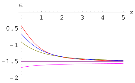
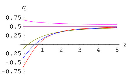
Figure 6: The slow roll parameter $\epsilon\equiv\dot{H}/H^{2}$ and deceleration parameter $q$ with respect to $z$, and $\alpha=0$, $0.7$, $1.0$, $1.48$, $1.6$ (from top to bottom, left plot) or (bottom to top, right plot).

         

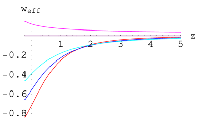
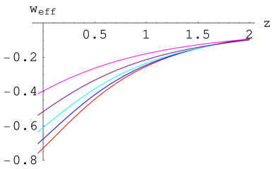
Figure 7: The effective EoS $w_{\lower 2.0pt\hbox{$\scriptstyle\rm eff$}}$ with respect to redshift $z$: (left plot) $\alpha=0$, $0.7$, $1.0$, $1.48$, $1.6$ (bottom to top) and (right plot) $\alpha=0$, $0.4$, $0.6$, $0.8$, $1.0$ (bottom to top).

         

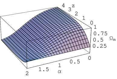
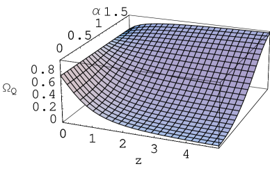
Figure 8: $\Omega_{\lower 2.0pt\hbox{$\scriptstyle m$}}$ and $\Omega_{\lower 2.0pt\hbox{$\scriptstyle Q$}}$ with respect to $\alpha$ and $z$. These quantities may not change with $z$ only if $\alpha=\alpha_{\lower 2.0pt\hbox{$\scriptstyle\rm crit$}}=1.48$, in which case obviously there won’t be a cosmic acceleration.

In Fig. 6, it can be easily seen that, for all $0\leq\alpha<1.48$, $q$ gets negative somewhen between redshifts $z=0$ and $z=1$, which implies that in this model accelerated expansion is a rather late time phenomenon with the universe getting into an accelerated phase the earliest for $\alpha\equiv 0$, corresponding to the cosmological constant case. In the case of $\alpha=1.48$, $q$ exactly equals $0.5$, corresponding to a decelerated expansion at constant deceleration. Finally, for $\alpha>\alpha_{\lower 2.0pt\hbox{$\scriptstyle\rm crit$}}=1.48$, $q$ is greater than $0.5$ and increases with decreasing redshift, yielding a decelerated expansion. This fits to the evolution of the dark energy EoS $w_{\lower 2.0pt\hbox{$\scriptstyle Q$}}$, as seen in Fig. 5 (for $\alpha>\alpha_{\lower 2.0pt\hbox{$\scriptstyle\rm crit$}}$, $w_{\lower 2.0pt\hbox{$\scriptstyle Q$}}>0$).

From Figs. 7 and 8 we can see that for the solution which leads to a late time acceleration ($w_{\lower 2.0pt\hbox{$\scriptstyle\rm eff$}}<-1/3$) the universe is clearly dominated at high redshift by $\Omega_{\rm m}$ with a transition to $\Omega_{{Q}}$ dominance in recent time leading to $\Omega_{\rm m}=0.27$ and $\Omega_{{Q}}=0.73$ at $z=0$. (That for sure does not come surprisingly, since that was the assumption made when fixing $c_{\lower 2.0pt\hbox{$\scriptstyle 1$}}$). It is perhaps more interesting to note that for $\alpha=1.48$ the ratio $\Omega_{\lower 2.0pt\hbox{$\scriptstyle Q$}}/\Omega_{\lower 2.0pt\hbox{$\scriptstyle m$}}$ remains constant for all $z$, whereas, for $\alpha<1.48$, the early universe would be dominated by $\Omega_{\lower 2.0pt\hbox{$\scriptstyle m$}}$ with a shift to dark energy dominance in the recent epoch. The observed acceleration and DE dominance correspond best to values of $\alpha$ closer to zero.

Uncertainties in the current value of $\Omega_{\lower 2.0pt\hbox{$\scriptstyle m$}}$ affect $\alpha_{\lower 2.0pt\hbox{$\scriptstyle\rm crit$}}$, to some extent, and hence the predicted value of $w_{\lower 2.0pt\hbox{$\scriptstyle Q$}}$ at some fixed redshift. That is, for a value of $\Omega_{\lower 2.0pt\hbox{$\scriptstyle m$}}$ different from $0.27$ at present, the critical value of $\alpha$, i.e. $\alpha_{\lower 2.0pt\hbox{$\scriptstyle\rm crit$}}=\sqrt{2.19}$, can also be different. However, the general bahaviour of the solution would be similar.

     

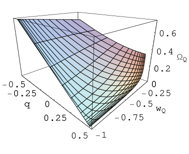
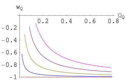
Figure 9: $\Omega_{{Q}}$ with respect to $w_{\lower 2.0pt\hbox{$\scriptstyle Q$}}$ and $q$, for a varying $z=\{5,0\}$ and $\alpha=\{1,0\}$ (left plot) and $\alpha=0$, $0.15$, $0.3$, $0.45$, $0.6$ (right plot, bottom to top). $w_{\lower 2.0pt\hbox{$\scriptstyle Q$}}$ lowers to $-1$ at a low redshift.

The left plot in Fig. 9 is a three-dimensional illustration of the above discussed fact, that a transition to the accelerated phase ($q<0$) occurs for $w_{\lower 2.0pt\hbox{$\scriptstyle Q$}}$ tending to $-1$ and $\Omega_{{Q}}$ tending to $+1$. The right plot in Fig. 9 is a two-dimensional projection of the latter and thus just gives another illustration of the already discussed relation between $w_{\lower 2.0pt\hbox{$\scriptstyle Q$}}$ and $\Omega_{{Q}}$ for the accelerating case, where only accelerating solutions with $\alpha<0.6$, which actually lead to $w_{\lower 2.0pt\hbox{$\scriptstyle Q$}}<-0.83$ at $z=0$, are examined.

         

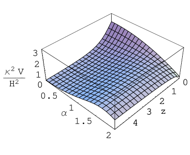
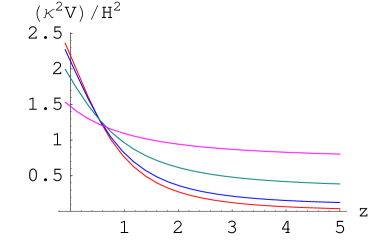
Figure 10: (Left plot) $\frac{\kappa^{2}\,V(Q)}{H^{2}(Q)}$ with respect to $z$ and $\alpha$. (Right plot) $\frac{\kappa^{2}\,V(Q)}{H^{2}(Q)}$ with respect to $z$ for $\alpha=0$, $0.4$, $0.8$ and $1.2$ (from bottom to top, at the right end of the graph).

The discussion so far has been based on the idea of a dark energy as described by the scalar field ${Q}$ with some potential $V(Q)$. For obtaining the analytical solution, (58)-(60), no particular choice was made for the potential. The only one assumption made was that the field might be rolling with a constant velocity $\alpha$, with respect to the e-folding time $N=\ln a$. Thus it would be worth looking at the shape of the potential as determined by this particular solution, following the idea of reconstruction underlying the focus of this paper. For obtaining the analytic expression of $V(Q)$, it is useful to consider the set of substitutions made in (36)-(37). By utilising the additional constraint (57), it is easy to see that

$$Y\equiv\frac{\kappa^{2}\,V(Q)}{H^{2}(Q)}=3\,\Omega_{{Q}}-\frac{\alpha^{2}}{2}.$$ (66)

$Y$ is actually a dimensionless variable, which takes the value $Y=3$ in a pure de Sitter space. The variation of $Y$ shown in Fig. 10 seems quite natural and can be understood in the following way. In order to get an accelerated expansion of the universe, with $w_{\lower 2.0pt\hbox{$\scriptstyle Q$}}$ close to $-1$ at a low redshift, $Y/3$ should exceed $\Omega_{\lower 2.0pt\hbox{$\scriptstyle m$}}$ in the recent past.

In order to find the potential, it is necessary first to evaluate the Hubble parameter $H$, which can be easily done by solving the equation

$$\epsilon[N]\,H[N]=H^{\prime}[N].$$ (67)

The analytic expression of $H$ is given by

$$H=c_{\lower 2.0pt\hbox{$\scriptstyle 2$}}\,\exp\left[\frac{-N\,\alpha^{2}}{2}\right]\sqrt{3\,\exp\left[-\lambda N\right]+c_{\lower 2.0pt\hbox{$\scriptstyle 1$}}\,\lambda},$$ (68)

The numerical constant $c_{\lower 2.0pt\hbox{$\scriptstyle 2$}}$ can be fixed by the assumption that $H[N=0]=H_{0}$. Hence

$$c_{\lower 2.0pt\hbox{$\scriptstyle 2$}}=\frac{H_{0}}{\sqrt{3+c_{\lower 2.0pt\hbox{$\scriptstyle 1$}}\,\lambda}}.$$ (69)

Finally, the quintessence potential takes the form

$$\kappa^{2}\,V(Q(N))=\frac{1}{2}\,c_{\lower 2.0pt\hbox{$\scriptstyle 2$}}^{2}\,\exp\left[-\,\alpha^{2}N\right]\,\left(3\alpha^{2}\,\exp\left[-\lambda N\right]+c_{\lower 2.0pt\hbox{$\scriptstyle 1$}}\,\left(18-9\,\alpha^{2}+\alpha^{4}\right)\right).$$ (70)

         

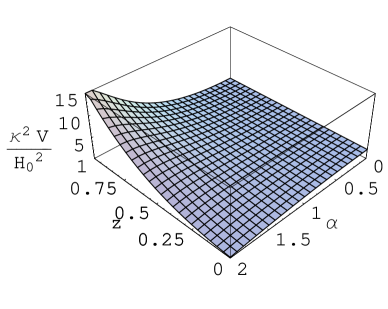
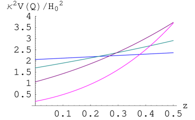
Figure 11: (Left plot) $\frac{\kappa^{2}\,V}{H_{0}^{2}}$ with respect to z and $\alpha$. (Right plot) $\frac{\kappa^{2}\,V}{H_{0}^{2}}$ with respect to $z$ for $\alpha=0.5$, $1.0$, $1.5$, $2.0$ (from top to bottom, along the y-axis).

In Fig. 11 it is clearly seen that $V(Q)$ increases exponentially with increasing redshift $z$, whereas this increment is more steep for larger values of $\alpha$. As it should be, in the $\alpha=0$ case, the potential takes a constant value. In fact, the assumption of ${Q}$ rolling with a constant velocity (${Q}^{\prime}\equiv\alpha$) yields that the potential $V(Q(z))$ must take a shape to cause this behaviour for $Q$. An exponential shape for the potential is no surprise. The quintessence potential constructed in this way takes the following form

$$\kappa^{2}V=\frac{c_{\lower 2.0pt\hbox{$\scriptstyle 2$}}^{2}}{2}\,e^{-\,\alpha\left(c_{\lower 2.0pt\hbox{$\scriptstyle 3$}}+\kappa\,{Q}\right)}\left(3\alpha^{2}\,\exp\left[\frac{\left(\alpha^{2}-3\right)\left(c_{\lower 2.0pt\hbox{$\scriptstyle 3$}}+\kappa{Q}\right)}{\alpha}\right]+c_{\lower 2.0pt\hbox{$\scriptstyle 1$}}\left(18-9\alpha^{2}+\alpha^{4}\right)\right).$$ (71)

The integration constant $c_{\lower 2.0pt\hbox{$\scriptstyle 3$}}$ can be set to zero, without loss of generality, while $c_{\lower 2.0pt\hbox{$\scriptstyle 1$}}$ and $c_{\lower 2.0pt\hbox{$\scriptstyle 2$}}$ can be fixed in terms of $\alpha$ (and $H_{0}$), using eqs. (64) and (69). The potential can be brought into a form where it only depends on ${Q}$ and $\alpha$:

$$V(Q)=m_{\lower 2.0pt\hbox{$\scriptstyle P$}}^{2}\,\exp\left(-\,\frac{\alpha Q}{m_{\lower 2.0pt\hbox{$\scriptstyle P$}}}\right)\left(V_{\lower 2.0pt\hbox{$\scriptstyle 0$}}\,\exp\left[\frac{\left(\alpha^{2}-3\right)Q}{\alpha\,m_{\lower 2.0pt\hbox{$\scriptstyle P$}}}\right]+V_{\lower 2.0pt\hbox{$\scriptstyle 1$}}\right).$$ (72)

This potential is clearly double exponential in form and it would find interesting applications even for the early universe. As discussed in [34], one may be required to have $\alpha<0.8$ in order to satisfy the bound on $\Omega_{\lower 2.0pt\hbox{$\scriptstyle Q$}}$ during big bang nucleosynthesis, namely $\Omega_{\lower 2.0pt\hbox{$\scriptstyle Q$}}(1~{}{\rm MeV})<0.1$. It is also interesting to note that such a potential can easily arise from some fundamental theories of gravity in higher dimensions (see e.g. [35]).

         

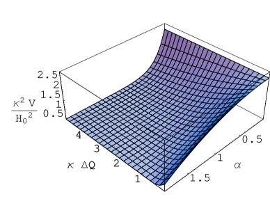
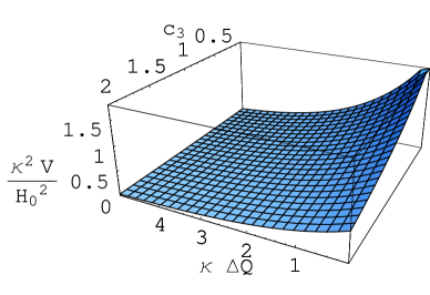
Figure 12: (Left plot) $\frac{\kappa^{2}\,V(Q)}{H_{0}^{2}}$ with respect to $\kappa\,{Q}$ and $\alpha$, for $c_{\lower 2.0pt\hbox{$\scriptstyle 3$}}=0$. (Right plot) $\frac{\kappa^{2}\,V(Q)}{H_{0}^{2}}$ with respect to $\kappa\,{Q}$ and $c_{\lower 2.0pt\hbox{$\scriptstyle 3$}}$, for $\alpha=0.6$.

The form of the potential, as it can be seen in Fig. 12, is not surprising, as it allows the field to “roll down” the slope of a decreasing $V(Q)$ for an increasing ${Q}$, or a decreasing redshift. As expected, the slope of the potential is shallower for smaller values of $\alpha$ and equals zero in the cosmological constant case, $\alpha\equiv 0$.

3.3 Coupled Quintessence

As already mentioned above, when solving the system of equations (52)-(55) with the additional constraint (57) in the general case ($\alpha_{\lower 2.0pt\hbox{$\scriptstyle Q$}}\neq 0$), one more constraint is needed to get an analytic solution. It is most canonical to assume $\kappa\,\alpha_{\lower 2.0pt\hbox{$\scriptstyle Q$}}\equiv const\equiv\chi$, which represents the case of so-called exponential coupling between the scalar field ${Q}$ and matter, as $A(Q)\propto{\rm e}^{\,\chi(Q/m_{\lower 2.0pt\hbox{$\scriptstyle P$}})}$. This additional assumption then leads to a general analytic solution

$$\Omega_{\lower 2.0pt\hbox{$\scriptstyle Q$}} = 1-\frac{\zeta}{3+c_{\lower 2.0pt\hbox{$\scriptstyle 4$}}\left(3+\alpha\chi-\alpha^{2}\right){\rm e}^{\zeta N}},$$ (73)

$$w_{\lower 2.0pt\hbox{$\scriptstyle Q$}} = \frac{c_{\lower 2.0pt\hbox{$\scriptstyle 4$}}\,\zeta\,\exp\left[\zeta N\right]\,\left(\alpha^{2}-3\right)+3\,\chi\alpha}{3c_{\lower 2.0pt\hbox{$\scriptstyle 4$}}\,\zeta\,\exp\left[\zeta N\right]+3\alpha^{2}-3\chi\alpha}$$ (74)

$$\epsilon = -\frac{\alpha^{2}}{2}+\frac{-3\zeta}{2c_{\lower 2.0pt\hbox{$\scriptstyle 4$}}\zeta\,\exp\left[\zeta N\right]+6},$$ (75)

where

$$\zeta\equiv 3+\chi\,\alpha-\alpha^{2},$$ (76)

Further, the analytic expressions for $q$ and $w_{\lower 2.0pt\hbox{$\scriptstyle\rm eff$}}$ are given by

$$q=-1+\frac{\alpha^{2}}{2}+\frac{3\zeta}{2c_{\lower 2.0pt\hbox{$\scriptstyle 4$}}\zeta\,\exp\left[\zeta N\right]+6}$$ (77)

$$w_{\lower 2.0pt\hbox{$\scriptstyle\rm eff$}}=-1+\frac{\alpha^{2}}{3}+\frac{2\zeta}{2c_{\lower 2.0pt\hbox{$\scriptstyle 4$}}\zeta\,\exp[\zeta N]+6}.$$ (78)

By solving the differential equation (67), the Hubble parameter is found to be

$$H(Q)=c_{\lower 2.0pt\hbox{$\scriptstyle 5$}}\,\exp\left[\frac{-\,N\left(3+\alpha\chi\right)}{2}\right]\sqrt{c_{\lower 2.0pt\hbox{$\scriptstyle 4$}}\,\zeta\,\exp\left[\zeta N\right]+3},$$ (79)

where $N\equiv N(Q)$. The integration constant $c_{\lower 2.0pt\hbox{$\scriptstyle 5$}}$ can be fixed by the assumption that $H[N=0]\equiv H_{0}$. This yields

$$c_{\lower 2.0pt\hbox{$\scriptstyle 5$}}=\frac{H_{0}}{\sqrt{3+c_{\lower 2.0pt\hbox{$\scriptstyle 4$}}\,\zeta}}.$$ (80)

One normalizes $N$ such that $N=0$ corresponds to $a\equiv a_{\lower 2.0pt\hbox{$\scriptstyle 0$}}=1$. Further, insisting that $\Omega_{\lower 2.0pt\hbox{$\scriptstyle\rm m$}}\left(N=0,\alpha,c_{\lower 2.0pt\hbox{$\scriptstyle 4$}},\chi\right)\equiv\Omega_{\lower 2.0pt\hbox{$\scriptstyle m$}}^{0}$ at $z=0$ fixes the integration constant $c_{\lower 2.0pt\hbox{$\scriptstyle 4$}}$ in terms of $\alpha$ and $\chi$:

$$c_{\lower 2.0pt\hbox{$\scriptstyle 4$}}=\frac{3(1-\Omega_{\lower 2.0pt\hbox{$\scriptstyle m$}}^{0})+\alpha\chi-\alpha^{2}}{\Omega_{\lower 2.0pt\hbox{$\scriptstyle m$}}^{0}(3+\alpha\chi-\alpha^{2})}.$$ (81)

Compared to the minimal coupling case ($\chi=0$), now the symmetry in the solution between positive and negative $\alpha$ is lost. However, a simultaneous change in sign of the parameters $\alpha$ and $\chi$ keeps $c_{\lower 2.0pt\hbox{$\scriptstyle 4$}}$ unchanged. Thus in further analysis only the properties of a solution with positive $\alpha$ but either sign of $\chi$ will be examined. In the discussion that follows the case $\chi<0$ will characterize solutions with $\alpha$ and $\chi$ having the opposite sign, while the case $\chi>0$ will characterize solutions with $\alpha$ and $\chi$ having the same sign.

As the parameters $q$, $w_{\lower 2.0pt\hbox{$\scriptstyle\rm eff$}}$ and $\epsilon$ are all intimately connected by eqs. (50) and (51), only the $\chi$-dependence of dark energy EoS $w_{\lower 2.0pt\hbox{$\scriptstyle Q$}}$ will be examined as an exemplary.

As can be seen from Fig. 13, the $\chi>0$ solution decreases $w_{\lower 2.0pt\hbox{$\scriptstyle Q$}}$, whereas the $\chi<0$ solution increases $w_{\lower 2.0pt\hbox{$\scriptstyle Q$}}$ (for fixed $\alpha$ and $z$). That is, a negative $\chi$ causes the universe to get into an accelerating phase later than for positive $\chi$. In general, the decrease in $w_{\lower 2.0pt\hbox{$\scriptstyle{Q}$}}$ would be steeper for $\chi<0$ than for $\chi\geq 0$. It is also important to realize that the coupling $\chi$ does not affect the value of $w_{\lower 2.0pt\hbox{$\scriptstyle Q$}}$ at $z\simeq 0$ but only at higher redshifts.

         

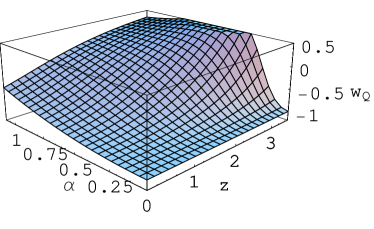
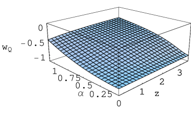
Figure 13: The dark energy equation of state $w_{\lower 2.0pt\hbox{$\scriptstyle Q$}}$ with respect to $z$ and $\alpha$ for $\chi=-0.4$ (left plot) and $\chi=+0.4$ (right plot). The $\chi>0$ solution yields a more negative $w_{\lower 2.0pt\hbox{$\scriptstyle Q$}}$ at a given redshift.

         

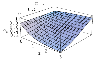
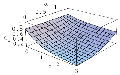
Figure 14: $\Omega_{\lower 2.0pt\hbox{$\scriptstyle Q$}}$ with respect to $z$ and $\alpha$ for $\chi=-0.6$ (left plot) and $\chi=+0.6$ (right plot).

In Fig. 14 we show the variation of dark energy density with the field velocity $\alpha$ and the redshift $z$. It is found that, for fixed $\alpha$ ($<\alpha_{\lower 2.0pt\hbox{$\scriptstyle\rm crit$}}$), $\Omega_{\lower 2.0pt\hbox{$\scriptstyle Q$}}$ can be smaller (larger) at higher redshifts for $\chi>0$ ($\chi<0$). This behavior would be somewhat opposite in an decelerating universe with $\alpha>\alpha_{\lower 2.0pt\hbox{$\scriptstyle\rm crit$}}$. This behaviour is expected by the $\chi$-dependence of $q$, since an increase in matter density also increases $q$ and vice versa. For a better understanding of this situation, it is useful to study the behaviour of the potential $V(Q)$.

It is also worth examining the values of dark energy EoS $w_{\lower 2.0pt\hbox{$\scriptstyle Q$}}$ with a varying $\chi$. In the case $\chi<0$, an increasing negative $\chi$ decreases $w_{\lower 2.0pt\hbox{$\scriptstyle Q$}}$, whereas an increasing positive $\chi$ will increase $w_{\lower 2.0pt\hbox{$\scriptstyle Q$}}$ with respect to the value it has in the minimal coupling case, $\chi=0$; one may compare the figure 15 with 5.

         

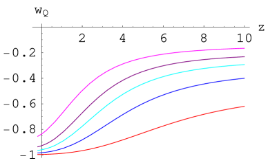
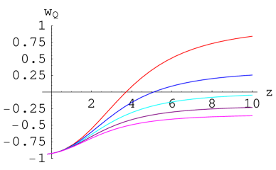
Figure 15: The dark energy EoS $w_{\lower 2.0pt\hbox{$\scriptstyle Q$}}$ with respect to $z$. Left plot: $\chi=+0.1$ and $\alpha=0$, $0.2$, $0.4$, $1.0$, $1.4$ (bottom to top). Right plot: $\alpha=0.4$ and $\chi=-0.2$, $-0.1$, $0$, $0.1$, $0.2$ (top to bottom).

In analogy to the previous section $\frac{\kappa^{2}\,V(Q)}{H^{2}(Q)}$ can be obtained by using eq. (66). In the $\chi\neq 0$ case, the effective potential consists of $V(Q)$ and an additional term depending on the matter-quintessence coupling $\alpha_{\lower 2.0pt\hbox{$\scriptstyle Q$}}$. The functional form of $V_{\lower 2.0pt\hbox{$\scriptstyle\rm eff$}}(Q)$ can be obtained by integrating the right hand side of eq. (33) with respect to $Q$. The result is given by

$$\kappa^{2}\,V_{\lower 2.0pt\hbox{$\scriptstyle\rm eff$}}(Q)=0.5\,c_{\lower 2.0pt\hbox{$\scriptstyle 5$}}^{2}\,\exp\left[\frac{-\left(3+\alpha\chi\right)\,\left(c_{\lower 2.0pt\hbox{$\scriptstyle 6$}}+\kappa\,{Q}\right)}{\alpha}\right]$$

$$\qquad\times\left(c_{\lower 2.0pt\hbox{$\scriptstyle 4$}}\,\zeta\,\exp\left[\frac{\zeta\,\left(c_{\lower 2.0pt\hbox{$\scriptstyle 6$}}+\kappa\,{Q}\right)}{\alpha}\right]\,\left(6-\alpha^{2}\right)-3\,\left(6+4\,\alpha\chi-3\,\alpha^{2}\right)\right),$$ (82)

where $c_{\lower 2.0pt\hbox{$\scriptstyle 6$}}$ is an integration constant. One can fix $c_{\lower 2.0pt\hbox{$\scriptstyle 4$}}$ and $c_{\lower 2.0pt\hbox{$\scriptstyle 5$}}$ using eqs. (81) and (80), and also eq. (65). We exhibit the shape of this potential in Fig. 16.

         

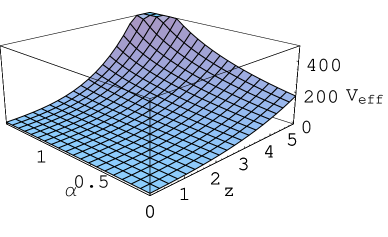
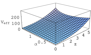
Figure 16: The effective potential $V_{\lower 2.0pt\hbox{$\scriptstyle\rm eff$}}(Q)$ with respect to redshift $z$ and the slope parameter $\alpha$, in the units $H_{\lower 2.0pt\hbox{$\scriptstyle 0$}}=1=\kappa$, for $\chi=-0.5$ (left plot) and $\chi=+0.5$ (right plot). We have taken $c_{\lower 2.0pt\hbox{$\scriptstyle 6$}}=0$.

As can be easily seen in Fig. 16, for a small $\alpha$ ($<\alpha_{\lower 2.0pt\hbox{$\scriptstyle\rm crit$}}$), $V_{\lower 2.0pt\hbox{$\scriptstyle\rm eff$}}(Q)$ increases with an increasing $z$, which allows the field to “roll down” with a constant velocity ${\alpha}$, with the slope being zero for $\alpha=0$, as in the $\chi=0$ case. For large $\alpha$ (like $\alpha\gtrsim\sqrt{2}$), instead, $V_{\lower 2.0pt\hbox{$\scriptstyle\rm eff$}}(Q)$ decreases with an increasing $z$. This should not come as a surprise; this behaviour has its origin in the value of $\alpha_{\lower 2.0pt\hbox{$\scriptstyle\rm crit$}}$ which is lowered for $\chi<0$. For a given $\alpha$, the slope of the potential is shallower for $\chi>0$ than for $\chi<0$, with vanishing difference at lower redshifts.

We conclude this section with the following two remarks. Firstly, in our model, it is possible that the current acceleration of the universe is only transient. This can easily happen, for $\alpha_{\lower 2.0pt\hbox{$\scriptstyle Q$}}<0$, when $\sum_{\lower 2.0pt\hbox{$\scriptstyle i$}}\int\alpha_{\lower 2.0pt\hbox{$\scriptstyle Q$}}(1-3w_{\lower 2.0pt\hbox{$\scriptstyle i$}})\tilde{\rho}_{\lower 2.0pt\hbox{$\scriptstyle i$}}\,dQ$ (where $\widetilde{\rho}_{\lower 2.0pt\hbox{$\scriptstyle i$}}\propto a^{-3-3w_{\lower 2.0pt\hbox{$\scriptstyle i$}}}$) becomes comparable to (or exceeds) $\kappa^{2}V(Q)$, making the effective potential almost vanishing (or negative).

Secondly, in the case both the ordinary and dark matter have same coupling with the quintessence field $Q$, current observational constraints (from Cassini experiments and the likes) only demand that $\alpha_{\lower 2.0pt\hbox{$\scriptstyle Q$}}^{2}<10^{-4}$, while this bound is significantly relaxed if dark matter can have much stronger coupling with $Q$. It should be the astrophysical observations that decide whether $\alpha_{\lower 2.0pt\hbox{$\scriptstyle Q$}}<0$ or $\alpha_{\lower 2.0pt\hbox{$\scriptstyle Q$}}>0$. The answer to this question can have interesting cosmological effects which we aim to study in future work.

4 Confronting models with data

In this section we confront our models with recent cosmological datasets (Supernova Legacy Survey (SNLS) and SNIa Gold06 datasets) following the methods discussed, for example, in refs. [36, 37].

In the minimal coupling case, since $\dot{\rho}_{\lower 2.0pt\hbox{$\scriptstyle Q$}}+3H(1+w_{\lower 2.0pt\hbox{$\scriptstyle Q$}})\rho_{\lower 2.0pt\hbox{$\scriptstyle Q$}}=0$ (i.e. $\rho_{\lower 2.0pt\hbox{$\scriptstyle Q$}}$ and $\rho_{\lower 2.0pt\hbox{$\scriptstyle m$}}$ are separately conserved), we get

$$\rho_{\lower 2.0pt\hbox{$\scriptstyle Q$}}=\rho_{\lower 2.0pt\hbox{$\scriptstyle Q0$}}\exp\left[3\int_{0}^{z}\frac{(1+w(z_{1}))}{1+z_{1}}dz_{1}\right].$$ (83)

Without any prior on $w(z_{1})$ or $\rho_{\lower 2.0pt\hbox{$\scriptstyle Q$}}$, it can be shown that [38]

$$H(z)=H_{\lower 2.0pt\hbox{$\scriptstyle 0$}}\left(\Omega_{\lower 2.0pt\hbox{$\scriptstyle m0$}}(1+z)^{3}+\Omega_{\lower 2.0pt\hbox{$\scriptstyle Q0$}}\exp\left[3\int_{0}^{\ln(1+z)}(1+w(z_{\lower 2.0pt\hbox{$\scriptstyle 1$}}))d\ln(1+z_{\lower 2.0pt\hbox{$\scriptstyle 1$}})\right]\right)^{1/2},$$ (84)

and

$$w_{\lower 2.0pt\hbox{$\scriptstyle Q$}}(z)=\frac{\frac{2}{3}(1+z)\frac{d\ln H}{dz}-1}{1-\frac{H_{\lower 2.0pt\hbox{$\scriptstyle 0$}}^{2}}{H^{2}}\Omega_{\lower 2.0pt\hbox{$\scriptstyle m0$}}(1+z)^{3}}.$$ (85)

In our model we have assumed that $m_{\lower 2.0pt\hbox{$\scriptstyle P$}}\dot{Q}/{H}\equiv\alpha$. In this particular case, with $w_{\lower 2.0pt\hbox{$\scriptstyle m$}}=0$, the Hubble parameter $H(z)$ as a function of the redshift $z$ is given by (cf eq. (68))

$$H(z) = H_{\lower 2.0pt\hbox{$\scriptstyle 0$}}\sqrt{\Omega_{\lower 2.0pt\hbox{$\scriptstyle m0$}}(1+z)^{3}+(1-\Omega_{\lower 2.0pt\hbox{$\scriptstyle m0$}})(1+z)^{\alpha^{2}}},$$ (86)

where $\Omega_{\lower 2.0pt\hbox{$\scriptstyle m0$}}\equiv 3/(3+\widetilde{c}_{\lower 2.0pt\hbox{$\scriptstyle 1$}})$. Using this expression of $H(z)$, we show in Fig. 17 the best fit form of $w(z)$ for the SNLS data with a prior $\Omega_{\lower 2.0pt\hbox{$\scriptstyle m0$}}=0.24$. The dark energy equation of state $w_{\lower 2.0pt\hbox{$\scriptstyle Q$}}(z)$ is given by

$$w_{\lower 2.0pt\hbox{$\scriptstyle Q$}}(z)=\frac{(1-\Omega_{\lower 2.0pt\hbox{$\scriptstyle m0$}})(\alpha^{2}-3)}{3(1-\Omega_{\lower 2.0pt\hbox{$\scriptstyle m0$}})+\alpha^{2}\Omega_{\lower 2.0pt\hbox{$\scriptstyle m0$}}(1+z)^{3-\alpha^{2}}}.$$ (87)

Clearly, knowledge of $\Omega_{\lower 2.0pt\hbox{$\scriptstyle m0$}}$ and $\alpha$ would suffice to determine $w_{\lower 2.0pt\hbox{$\scriptstyle Q$}}(z)$. In the $\alpha=0$ case, $w_{\lower 2.0pt\hbox{$\scriptstyle Q$}}(z)=w_{\lower 2.0pt\hbox{$\scriptstyle\Lambda$}}=-1$. In tables 1 and 2 we present the best fit values of $\alpha$ and $w_{\lower 2.0pt\hbox{$\scriptstyle Q$}}$ for different choices of $\Omega_{\lower 2.0pt\hbox{$\scriptstyle m0$}}$.

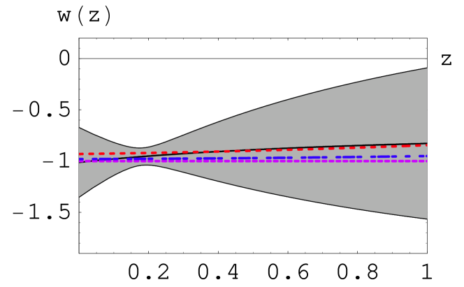
Figure 17: The best fit form of $w(z)$ for the SNLS datasets for a prior of $\Omega_{\lower 2.0pt\hbox{$\scriptstyle m0$}}=0.24$ along with the $1\sigma$ errors (shaded region). The (black) solid line corresponds to the ansatz $w(z_{\lower 2.0pt\hbox{$\scriptstyle 1$}})\equiv w_{\lower 2.0pt\hbox{$\scriptstyle 0$}}+w_{\lower 2.0pt\hbox{$\scriptstyle 1$}}z_{\lower 2.0pt\hbox{$\scriptstyle 1$}}/(1+z_{\lower 2.0pt\hbox{$\scriptstyle 1$}})$ (cf eq. (85)). The three other lines correspond to $\alpha=0.4,0.2109,0$ (top to bottom) and $w_{\lower 2.0pt\hbox{$\scriptstyle Q$}}(z)$ given by eq. (87). With $\Omega_{\lower 2.0pt\hbox{$\scriptstyle m0$}}=0.24$, $\alpha=0.2109$ minimizes the $\chi_{\lower 2.0pt\hbox{$\scriptstyle min$}}^{2}$ ($=104.18$). The SNLS data may favour a lower value of $\Omega_{\lower 2.0pt\hbox{$\scriptstyle m0$}}$ (as compared to the Gold SNIa dataset). Further, with a canonical quintessence, so that $w_{\lower 2.0pt\hbox{$\scriptstyle Q$}}(z=0)\gtrsim-1$, we may require $\Omega_{\lower 2.0pt\hbox{$\scriptstyle m0$}}<0.2592$.

Table 1: The best fit values of $w_{\lower 2.0pt\hbox{$\scriptstyle Q$}}(z)$ and $\alpha$ for the SNLS datasets for a given $\Omega_{\lower 2.0pt\hbox{$\scriptstyle m0$}}$. $\Omega_{\lower 2.0pt\hbox{$\scriptstyle m0$}}$ $|\alpha|$ $w_{\lower 2.0pt\hbox{$\scriptstyle Q$}}(z=0)$ $\chi_{\lower 2.0pt\hbox{$\scriptstyle min$}}^{2}$ $0.22$ $0.2948$ $-0.9628$ $104.23$ $0.23$ $0.2573$ $-0.9713$ $104.21$ $0.24$ $0.2109$ $-0.9805$ $104.18$ $0.25$ $0.1476$ $-0.9903$ $104.16$ $0.259173$ $0.014$ $-0.9999$ $104.14$

Table 2: The best fit values of $w_{\lower 2.0pt\hbox{$\scriptstyle Q$}}(z)$ and $\alpha$ for the Gold SNIa dataset for a given $\Omega_{\lower 2.0pt\hbox{$\scriptstyle m0$}}$. $\Omega_{\lower 2.0pt\hbox{$\scriptstyle m0$}}$ $|\alpha|$ $w_{\lower 2.0pt\hbox{$\scriptstyle Q$}}(z=0)$ $\chi_{\lower 2.0pt\hbox{$\scriptstyle min$}}^{2}$ $0.23$ $0.4001$ $-0.9307$ $178.64$ $0.25$ $0.3376$ $-0.9493$ $178.21$ $0.27$ $0.2544$ $-0.9704$ $177.76$ $0.29$ $0.0933$ $-0.9959$ $177.31$ $0.2929$ $0.0100$ $-0.9999$ $177.25$

The Gold SNIa datasets could actually fit better with coupled quintessence (or interacting dark energy) models (cf Fig. 18).

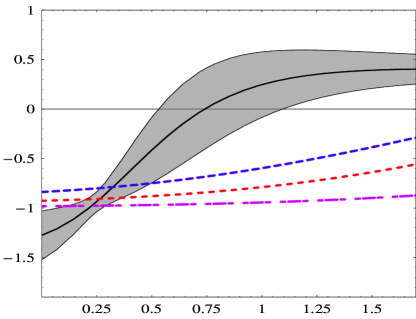
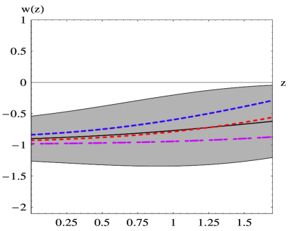
Figure 18: The best fit form of $w(z)$ for the Gold SNIa dataset for a prior of $\Omega_{\lower 2.0pt\hbox{$\scriptstyle m0$}}=0.27$ along with the $1\sigma$ errors (shaded region) with $H(z)$ given by eq. (89) (left plot) and $H_{\lower 2.0pt\hbox{$\scriptstyle\rm obs$}}(z)$ given by (92) (right plot); $\chi^{2}$ is minimized for $\alpha=0.4735$ and $\alpha_{\lower 2.0pt\hbox{$\scriptstyle Q_{0}$}}=0.0633$. The (black) solid line corresponds to the best fit line with $\chi_{\lower 2.0pt\hbox{$\scriptstyle min$}}^{2}$($\simeq 177$) and the three other lines represent $w_{\lower 2.0pt\hbox{$\scriptstyle Q$}}(z)$ (cf eq. (90)) with $\alpha=0.6,0.4,0.2$ (top to bottom) and $\alpha_{\lower 2.0pt\hbox{$\scriptstyle Q$}}\equiv\chi=0.4$.

In the non-minimal coupling case, $\rho_{\lower 2.0pt\hbox{$\scriptstyle Q$}}$ is not separately conserved, since $\dot{\rho}_{\lower 2.0pt\hbox{$\scriptstyle Q$}}+3H(1+w_{\lower 2.0pt\hbox{$\scriptstyle Q$}})\rho_{\lower 2.0pt\hbox{$\scriptstyle Q$}}=\alpha_{\lower 2.0pt\hbox{$\scriptstyle Q$}}HQ^{\prime}\rho_{\lower 2.0pt\hbox{$\scriptstyle m$}}$; of course, the total energy is always conserved: $\dot{\rho}_{\lower 2.0pt\hbox{$\scriptstyle\rm tot$}}+3H(\rho_{\rm tot}+p_{\lower 2.0pt\hbox{$\scriptstyle\rm tot$}})=0$, where $\rho_{\lower 2.0pt\hbox{$\scriptstyle\rm tot$}}=\rho_{\lower 2.0pt\hbox{$\scriptstyle m$}}+\rho_{\lower 2.0pt\hbox{$\scriptstyle Q$}}$. Using the relations $\partial/\partial t=H(\partial/\partial\ln a)$ and $\ln a=-\ln(1+z)$, we get

$$\rho_{\lower 2.0pt\hbox{$\scriptstyle Q$}}=\exp\left[3\int_{0}^{z}\frac{(1+w(z_{1}))}{1+z_{1}}dz_{1}\right]\left(\rho_{\lower 2.0pt\hbox{$\scriptstyle Q0$}}+\int_{0}^{z}\frac{Q^{\prime}\alpha_{\lower 2.0pt\hbox{$\scriptstyle Q$}}\rho_{m}}{1+z_{1}}\exp\left[-3\int_{0}^{z}\frac{(1+w(z_{1}))}{1+z_{1}}dz_{1}\right]dz_{1}\right).$$

In particular, with $m_{\lower 2.0pt\hbox{$\scriptstyle P$}}Q^{\prime}\equiv\alpha$ and $\alpha_{\lower 2.0pt\hbox{$\scriptstyle Q$}}=\frac{d\ln A(Q)}{d(\kappa Q)}\equiv\chi$, the Hubble parameter $H(z)$ is found to be

$$H(z)=H_{\lower 2.0pt\hbox{$\scriptstyle 0$}}\sqrt{\Omega_{\lower 2.0pt\hbox{$\scriptstyle m0$}}(1+z)^{3+\alpha\chi}+(1-\Omega_{\lower 2.0pt\hbox{$\scriptstyle m0$}})(1+z)^{\alpha^{2}}},$$ (89)

where $\Omega_{\lower 2.0pt\hbox{$\scriptstyle m0$}}\equiv 3/(3+\widetilde{c}_{\lower 2.0pt\hbox{$\scriptstyle 4$}}\zeta)$ and $\zeta\equiv 3-\alpha^{2}+\alpha\chi$. The dark energy equation of state is

$$w_{\lower 2.0pt\hbox{$\scriptstyle Q$}}(z)=\frac{\alpha\chi\Omega_{\lower 2.0pt\hbox{$\scriptstyle m0$}}+(1-\Omega_{\lower 2.0pt\hbox{$\scriptstyle m0$}})(\alpha^{2}-3)(1+z)^{-\zeta}}{3(1-\Omega_{\lower 2.0pt\hbox{$\scriptstyle m0$}})(1+z)^{-\zeta}+\alpha(\alpha-\chi)\Omega_{\lower 2.0pt\hbox{$\scriptstyle m0$}}}.$$ (90)

Next we briefly discuss about an interesting possibility (leaving the details and further generalization to a forthcoming paper). In the non-minimal coupling case, the Hubble expansion parameter that one measures (in a physical Jordan frame) could actually be different than the one given by (89) by a conformal factor. Given that

$$\frac{H_{\lower 2.0pt\hbox{$\scriptstyle\rm obs$}}(z)}{H(z)}=\exp[\chi(Q/m_{\lower 2.0pt\hbox{$\scriptstyle P$}})]\propto\exp[\chi\alpha\ln a]=a^{\alpha\chi}=(1+z)^{-\alpha\chi},$$ (91)

we find

$$H_{\lower 2.0pt\hbox{$\scriptstyle\rm obs$}}(z)={H}_{\lower 2.0pt\hbox{$\scriptstyle 0$}}\sqrt{\Omega_{\lower 2.0pt\hbox{$\scriptstyle m0$}}(1+z)^{3}+(1-\Omega_{\lower 2.0pt\hbox{$\scriptstyle m0$}})(1+z)^{\alpha^{2}-\alpha\chi}}.$$ (92)

Using this expression of $H(z)$, we have presented in table 3 the best fit values of $\alpha$ and $\alpha_{\lower 2.0pt\hbox{$\scriptstyle Q_{0}$}}$ which minimize the $\chi^{2}$ for the Gold SNIa, SNIa+CMB-shift (WMAP)+ SDSS data sets for a given $\Omega_{\lower 2.0pt\hbox{$\scriptstyle m0$}}\equiv 0.27$.

Table 3: The best fit values of $\alpha$ and $\alpha_{\lower 2.0pt\hbox{$\scriptstyle Q0$}}$, with $1\sigma$ errors for $w_{\lower 2.0pt\hbox{$\scriptstyle Q_{0}$}}\equiv w_{\lower 2.0pt\hbox{$\scriptstyle Q$}}(z=0)$.

	$\alpha$	$\alpha_{\lower 2.0pt\hbox{$\scriptstyle Q_{0}$}}$	$w_{\lower 2.0pt\hbox{$\scriptstyle Q_{0}$}}$ (eq. (90))	$w_{\lower 2.0pt\hbox{$\scriptstyle Q_{0}$}}$ (eq. (85))
SNIa	$0.4735$	$0.0633$	$-0.90^{+0.35}_{-0.33}$	$-0.94^{+0.10}_{-0.10}$
SNIa+WMAP+SDSS	$0.5142$	$0.0583$	$-0.88^{+0.26}_{-0.31}$	$-0.92^{+0.07}_{-0.08}$

The mean value of $w_{\lower 2.0pt\hbox{$\scriptstyle Q_{0}$}}$ obtained above is within the range indicated by WMAP3+SDSS observations: $w_{\lower 2.0pt\hbox{$\scriptstyle\rm DE$}}=-0.941^{+0.087}_{-0.101}$ [3]. The best fit value of $\alpha_{\lower 2.0pt\hbox{$\scriptstyle Q$}}$ is found to be $\alpha_{\lower 2.0pt\hbox{$\scriptstyle Q$}}\simeq 0.06$, but in our model it may contain significant numerical errors, namely $\alpha_{\lower 2.0pt\hbox{$\scriptstyle Q$}}=0.06\pm 0.35$, which thereby implies the consistency of our model with general relativity (for which $\alpha_{\lower 2.0pt\hbox{$\scriptstyle Q$}}=0$) at $1\sigma$ level. To illustrate this result we show in Fig. 19 the best fit plot with $\alpha_{\lower 2.0pt\hbox{$\scriptstyle Q$}}=0$.

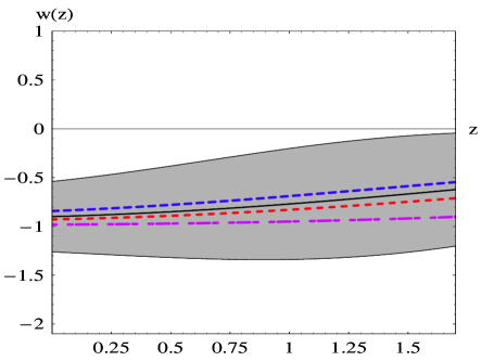
Figure 19: As in Fig.18 (right plot) but with $\alpha_{\lower 2.0pt\hbox{$\scriptstyle Q$}}=0$.

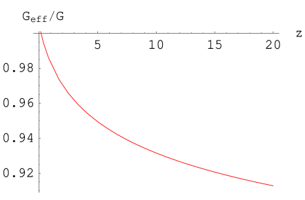
Figure 20: The time variation of Newton’s constant in the non-minimal case.

The post-Newtonian parameter $\tilde{\gamma}$ is related to $\alpha_{\lower 2.0pt\hbox{$\scriptstyle Q_{0}$}}$ ($\equiv\chi$) through the relation [39]

$$\alpha_{\lower 2.0pt\hbox{$\scriptstyle Q_{0}$}}^{2}=\frac{1-\tilde{\gamma}}{1+\tilde{\gamma}}.$$

With the best fit value $\alpha_{\lower 2.0pt\hbox{$\scriptstyle Q_{0}$}}\simeq 0.06$, this yields $|\tilde{\gamma}-1|\simeq 7.1\times 10^{-3}$, which is not far from a constraint coming from the Solar-system experiments, i.e., $|\tilde{\gamma}-1|<2\times 10^{-3}$. Moreover, in the non-minimal coupling case, with $A(Q)=e^{\chi(Q/m_{\lower 2.0pt\hbox{$\scriptstyle P$}})}$ ($\chi\neq 0$) and $Q(t)\equiv\alpha\ln a+{\rm const}$, there arise constraints on the time variation of Newton’s constant. With a scalar field $Q$ conformally coupled to the matter, the effective Newton’s constant (measured, e.g., in a Cavendish type experiment) can be given by

$$\frac{G_{\lower 2.0pt\hbox{$\scriptstyle\rm eff$}}}{G}=A(Q)^{2}\left(1+\alpha_{\lower 2.0pt\hbox{$\scriptstyle Q$}}^{2}\right)=(1+z)^{-\alpha\chi}(1+\chi^{2}).$$ (93)

The time derivative of Newton’s constant generally depends on the coupling $A(Q)$ and its derivative, $\alpha_{\lower 2.0pt\hbox{$\scriptstyle Q$}}$. In our model, with $\alpha\chi>0$, the case of decreasing $w_{\lower 2.0pt\hbox{$\scriptstyle Q$}}(z)$ (at a lower redshift) corresponds to an increasing Newton’s constant that boosts cosmic acceleration.

For the SNIa best fit value $(\alpha,\alpha_{\lower 2.0pt\hbox{$\scriptstyle Q$}})=(0.4735,0.0633)$, the variation of $G_{\lower 2.0pt\hbox{$\scriptstyle\rm eff$}}$ in the redshift range $z=\{0,20\}$ is less than $10\%$ (cf Fig. 20) and $|\frac{dG_{\lower 2.0pt\hbox{$\scriptstyle\rm eff$}}}{dt}|/G_{\lower 2.0pt\hbox{$\scriptstyle\rm eff$}}=0.029hH_{\lower 2.0pt\hbox{$\scriptstyle 0$}}\simeq 2.1\times 10^{-12}{\rm yr}^{-1}$. We should mention that the current solar system constraint on $\dot{G}_{\lower 2.0pt\hbox{$\scriptstyle\rm eff$}}/G_{\lower 2.0pt\hbox{$\scriptstyle\rm eff$}}$ could be more stringent than this, namely $(dG_{\lower 2.0pt\hbox{$\scriptstyle\rm eff$}}/dt)/G_{\lower 2.0pt\hbox{$\scriptstyle\rm eff$}}<10^{-13}~{}{\rm yr}^{-1}$ (see, e.g. ref. [40] which derives constraints on $\dot{G}/G$ and $\ddot{G}/G$ for a model where $Q$-field is explicitly coupled to the Einstein-Hilbert term); it is because the relevant background when studying the solar system is not the cosmological but the solution of (33) corresponding to the galactic environment, where $\dot{Q}/H\approx 0$ and $\rho_{\lower 2.0pt\hbox{$\scriptstyle\rm gal$}}\gg\rho_{\lower 2.0pt\hbox{$\scriptstyle\rm crit$}}\equiv 3H_{\lower 2.0pt\hbox{$\scriptstyle 0$}}^{2}/8\pi G$. In order to properly address the question of time derivative (or variation) of Newton’s constant, one has to consider in detail the dynamical system where $\alpha_{\lower 2.0pt\hbox{$\scriptstyle Q$}}$ is time-varying. This is left for future studies.

5 Conclusion

In this paper we have outlined construction of an effective cosmological model each for inflation and dark energy (or quintessence), within the framework of the standard scalar-tensor theory. The general assumption has been that the evolution of our universe can be described by Einstein’s gravity coupled to a fundamental scalar field plus matter, described by the general action (22). The gravitational part of the action, which is important for constructing a model of inflation, contains a scalar field lagrangian. The matter part of the action contains all possible matter constituents in the form of a perfect fluid plus a coupling term $A({Q})$ which characterizes a universal coupling between a fundamental scalar field $Q$ and ordinary (plus dark) matter.

In Section 2, we have presented an explicit model for inflation, by constructing an inflationary potential that, with proper choice of slope parameters, satisfies the main observational constraints from WMAP data, including the spectral index of scalar perturbations and tensor-to-scalar ratio.

In Section 3, we have first derived a set of autonomous equations, by utilizing a fundamental variational principle, that in a compact form describes the evolution of different cosmological parameters, namely $\Omega_{\lower 2.0pt\hbox{$\scriptstyle Q$}}$, $w_{\lower 2.0pt\hbox{$\scriptstyle Q$}}$, $\Omega_{\lower 2.0pt\hbox{$\scriptstyle i$}}$, $w_{\lower 2.0pt\hbox{$\scriptstyle i$}}$, $\epsilon$ and $\alpha_{\lower 2.0pt\hbox{$\scriptstyle Q$}}$, as a system of four differential equations, of which only three are linearly independent (cf (38) - (41)). By further general considerations, we have shown how the parameters $q$ and $w_{\lower 2.0pt\hbox{$\scriptstyle\rm eff$}}$ can be determined from a solution of the above system. As discussed in the body of text, the system of equations (38)-(41) could be analytically solved only by making a reduction in the number of free parameters or by imposing additional constraints. In this work, one of our aims was to keep the model as general as possible, but for being able to find analytic solutions the number of parameters was restricted to four, neglecting the radiation component, and making a reasonable additional assumption that ${Q}\equiv\alpha\ln a+{\rm const}$ at the present epoch.

First by examining the case with minimal coupling, $A(Q)=1$, a class of exact (analytical) solutions has been found (cf eqs. (58)-(63)), which find interesting applications for the present-day cosmology. The general solution found in the minimal coupling case has the behavior that it is independent of the sign of $\alpha$ (i.e. the sign of $\dot{Q}$). Thus the direction of a “rolling” scalar field ${Q}$ does not seem to have any significant effect (which also directly followed when looking at the scalar field Lagrangian (cf eq. (22)), except in the shape of the potential. It is found that the critical value $\alpha_{\lower 2.0pt\hbox{$\scriptstyle\rm crit$}}=1.48$ separates the parameter spaces of $\alpha$ such that $\alpha<\alpha_{\lower 2.0pt\hbox{$\scriptstyle\rm crit$}}$ allows a late time acceleration while $\alpha>\alpha_{\lower 2.0pt\hbox{$\scriptstyle\rm crit$}}$ does not. Thus the characteristic of the scalar field ${Q}$ acting as an additional self-repulsive or self-attractive form of energy is merely determined by the magnitude of the velocity of the field, $d(\kappa Q)/d\ln a\equiv\alpha$. In several interesting cases we have found a closed form expression for (reconstructed) quintessence potential $V(Q)$.

As the combination of WAMP and type Ia supernova observations show a significant constraint on the present-day DE equation of state, $w_{\lower 2.0pt\hbox{$\scriptstyle Q$}}=-0.941^{+0.087}_{-0.101}$; for the mean value $\omega_{\lower 2.0pt\hbox{$\scriptstyle Q$}}\sim-0.941$, we require $|\alpha|\sim 0.4207\sqrt{\Omega_{\lower 2.0pt\hbox{$\scriptstyle Q$}}}\sim 0.36$, while the WMAP+SSS bound $1\leq w_{\lower 2.0pt\hbox{$\scriptstyle Q$}}<-0.82$ may be satisfied for $|\alpha|<0.62$. Of course, $\alpha=0$ simply represents the cosmological constant case ($w_{\lower 2.0pt\hbox{$\scriptstyle Q$}}=-1$). Claiming the same range of $-1\leq w_{\lower 2.0pt\hbox{$\scriptstyle Q$}}<-0.82$ for $w_{\lower 2.0pt\hbox{$\scriptstyle Q$}}$ at redshift $z\gtrsim 0$ imposes a more restrictive constraint on the slope of the potential $\alpha$ being smaller than $0.6$. When looking at the evolution of different cosmological parameters ($\Omega_{\lower 2.0pt\hbox{$\scriptstyle Q$}}$, $\Omega_{\lower 2.0pt\hbox{$\scriptstyle\rm m$}}$, $w_{\lower 2.0pt\hbox{$\scriptstyle Q$}}$, $\epsilon$, $w_{\lower 2.0pt\hbox{$\scriptstyle\rm eff$}}$, $q$), we find that, for smaller values of $\alpha$, the model shows a late time accelerated expansion (for $z<1$), while a matter dominance at early times. These features are in agreement with recent WMAP and supernova observations.

To see how a non-minimal coupling, $\alpha_{\lower 2.0pt\hbox{$\scriptstyle Q$}}\neq 0$, might affect the cosmic expansion, we studied the simplest case of an exponential coupling $A({Q})\propto e^{\chi(Q/m_{\lower 2.0pt\hbox{$\scriptstyle P$}})}$, which implies $\alpha_{\lower 2.0pt\hbox{$\scriptstyle Q$}}\equiv\chi$. In this case the solution is found to have a dependenc on the sign of the slope parameter $\alpha$ and the coupling $\alpha_{\lower 2.0pt\hbox{$\scriptstyle Q$}}$. A replacement of $\alpha$ by $-\alpha$ is found to be equivalent to the replacement of $\alpha_{\lower 2.0pt\hbox{$\scriptstyle Q$}}$ by $-\alpha_{\lower 2.0pt\hbox{$\scriptstyle Q$}}$. Moreover, a positive coupling is found to decreases the dark energy equation of state $w_{\lower 2.0pt\hbox{$\scriptstyle Q$}}$, with respect to its value in the $\alpha_{\lower 2.0pt\hbox{$\scriptstyle Q$}}=0$ case, while this effect is opposite for $\alpha_{\lower 2.0pt\hbox{$\scriptstyle Q$}}<0$. Thus, for a fixed $\alpha$, the $\alpha_{\lower 2.0pt\hbox{$\scriptstyle Q$}}>0$ solution could make the energy represented by ${Q}$ more repulsive, as compared to the $\alpha_{\lower 2.0pt\hbox{$\scriptstyle Q$}}=0$ case. The coupling dependence of other parameters just resemble this fact ($\alpha_{\lower 2.0pt\hbox{$\scriptstyle Q$}}>0$ in our convention just means $\alpha$ and $\alpha_{\lower 2.0pt\hbox{$\scriptstyle Q$}}$ having the same sign). For $|\alpha_{\lower 2.0pt\hbox{$\scriptstyle Q$}}|\lesssim 0.1$, and at low redshifts, the present-day values of the cosmological parameters showed almost no $\alpha_{\lower 2.0pt\hbox{$\scriptstyle Q$}}$-dependence. That is, an observable effect on the evolution of cosmological parameters, such as $w_{\lower 2.0pt\hbox{$\scriptstyle\rm eff$}}$ and $\Omega_{Q}$ can be expected to be seen only for a strong matter-scalar coupling, like $|\alpha_{\lower 2.0pt\hbox{$\scriptstyle Q$}}|\gg 0.1$. The type Ia supernova data may favor a small value for matter-quintessence coupling, like $\alpha_{\lower 2.0pt\hbox{$\scriptstyle Q$}}\sim 0.06$.

We have also shown how in principle a non-minimal matter-scalar coupling can alter the evolution of the cosmological parameters. In general the coupling $\alpha_{\lower 2.0pt\hbox{$\scriptstyle Q$}}$ always appears in combination with the matter density $\rho_{\lower 2.0pt\hbox{$\scriptstyle m$}}$ (cf eq. (55)). As the mass of the scalar field ${Q}$ can be determined by $\left(d^{2}\,V_{\lower 2.0pt\hbox{$\scriptstyle\rm eff$}}/{d{Q}^{2}}\right)^{1/2}$ evaluated at a local minimum and the scalar-matter coupling in $V_{\lower 2.0pt\hbox{$\scriptstyle\rm eff$}}(Q)$ can involve a $\rho_{\lower 2.0pt\hbox{$\scriptstyle m$}}$-dependent term, the mass of a scalar field depends, in principle, on the ambient matter distribution. Thus in a more sophisticated model, not treating matter as an isotropic perfect fluid, the mass of the scalar field can vary locally due to a possibly strong local variation of $\rho_{\lower 2.0pt\hbox{$\scriptstyle m$}}$ on small scales.

Appendix A Appendix:

Corresponding to the action (22), the equations of motion that describe gravity, the scalar field $Q$ and the background fields (matter and radiation) are given by

$$\frac{1}{2\,\kappa^{2}}\left(R_{\mu\nu}-\frac{1}{2}g_{\mu\nu}R\right)-\frac{1}{2}\left(\nabla_{\mu}{Q}\nabla_{\nu}{Q}\right)+\frac{1}{4}\left(\nabla{Q}\right)^{2}g_{\mu\nu}+\frac{1}{2}V\left({Q}\right)g_{\mu\nu}-\frac{1}{2}A^{4}\left({Q}\right)T_{\mu\nu}=0,$$ (A.1)

$$\nabla_{\mu}\,\left(g^{\mu\nu}\,\nabla_{\nu}\,{Q}\right)-\frac{dV\left({Q}\right)}{d{Q}}+A^{3}\,\frac{dA\left({Q}\right)}{d{Q}}\,\sum_{i}\left(1-3\,w_{\lower 2.0pt\hbox{$\scriptstyle i$}}\right)\rho_{\lower 2.0pt\hbox{$\scriptstyle i$}}=0.$$ (A.2)

These equations may be supplemented with the equation of motion of a barotropic perfect fluid, which is given by

$$\frac{d\left(A^{4}\,\rho_{\lower 2.0pt\hbox{$\scriptstyle i$}}\right)}{d\left(a\,A\right)}=\left(A^{4}\,\dot{\rho_{\lower 2.0pt\hbox{$\scriptstyle i$}}}\,\frac{1}{\left(\dot{a}\,A\right)}+A^{3}\,\frac{\partial A}{\partial{Q}}\,\left(1-3\,w_{\lower 2.0pt\hbox{$\scriptstyle i$}}\right)\,\rho_{\lower 2.0pt\hbox{$\scriptstyle i$}}\,\dot{{Q}}\,\frac{1}{\left(\dot{a}\,A\right)}\right).$$ (A.3)

Combining the $(tt)$ and $(xx)$ components of the equation (A.1), we get

$$-2\,\dot{H}=\kappa^{2}\left(\frac{1}{2}\,\dot{{Q}}^{2}+V\left({Q}\right)+\frac{1}{2}\,\dot{{Q}}^{2}-V\left({Q}\right)+A^{4}\sum_{i}\left(\rho_{\lower 2.0pt\hbox{$\scriptstyle i$}}+w_{\lower 2.0pt\hbox{$\scriptstyle i$}}\rho_{\lower 2.0pt\hbox{$\scriptstyle i$}}\right)\right).$$ (A.4)

Dividing this equation by $H^{2}$ and then using the substitution in (37), yields

$$-\frac{2\,\dot{H}}{H^{2}}=\frac{\kappa^{2}\rho_{{Q}}}{H^{2}}+w_{\lower 2.0pt\hbox{$\scriptstyle Q$}}\,\frac{\kappa^{2}\rho_{{Q}}}{H^{2}}+\sum_{i}\left(\frac{\kappa^{2}A^{4}\rho_{\lower 2.0pt\hbox{$\scriptstyle i$}}}{H^{2}}\,\left(1+w_{\lower 2.0pt\hbox{$\scriptstyle i$}}\right)\right).$$ (A.5)

Multiplying eq. (32) with $\dot{{Q}}$ and using the identities

$$\dot{\rho}_{\lower 2.0pt\hbox{$\scriptstyle Q$}}=\dot{Q}\ddot{Q}+\dot{V},\quad\rho_{\lower 2.0pt\hbox{$\scriptstyle Q$}}\left(1+w_{Q}\right)=\dot{{Q}}^{\,2},$$ (A.6)

which follow from eq. (37), we get

$$\dot{\rho}_{\lower 2.0pt\hbox{$\scriptstyle Q$}}+3H\rho_{\lower 2.0pt\hbox{$\scriptstyle Q$}}\,\left(1+w_{\lower 2.0pt\hbox{$\scriptstyle Q$}}\right)=\dot{Q}\,A^{3}\,\frac{dA\left({Q}\right)}{d{Q}}\,\sum_{i}\left(1-3\,w_{\lower 2.0pt\hbox{$\scriptstyle i$}}\right)\,\rho_{\lower 2.0pt\hbox{$\scriptstyle i$}}.$$ (A.7)

Multiplying (A.7) by $\frac{\kappa^{2}}{3H^{2}}$ and then using equations (42) and (36)-(37) leads to eq. (40). Further, multiplying eq. (35) by $\frac{\kappa^{2}}{3H^{2}}$ and then using eq. (42) leads to

$$\frac{\kappa^{2}\rho_{\lower 2.0pt\hbox{$\scriptstyle i$}}^{\prime}}{3H^{2}}+\frac{\kappa^{2}\rho_{\lower 2.0pt\hbox{$\scriptstyle i$}}}{3H^{2}}\left(1+w_{\lower 2.0pt\hbox{$\scriptstyle i$}}\right)=\frac{\kappa^{2}\,{Q}^{\,\prime}}{3H^{2}}\,\frac{\frac{dA\left({Q}\right)}{d{Q}}}{A\left({Q}\right)}\left(1-3w_{\lower 2.0pt\hbox{$\scriptstyle i$}}\right)\rho_{\lower 2.0pt\hbox{$\scriptstyle i$}}.$$ (A.8)

Combining this equation with the identity

$$\Omega_{\lower 2.0pt\hbox{$\scriptstyle i$}}^{\prime}\equiv\frac{\kappa^{2}\,A^{4}}{3\,H^{2}}\,\rho_{\lower 2.0pt\hbox{$\scriptstyle i$}}^{\prime}-2\,\epsilon\,\Omega_{\lower 2.0pt\hbox{$\scriptstyle i$}},$$ (A.9)

and then using the substitutions in (36)-(37), finally gives equation (41).

References

[1]
A. G. Riess et al. [Supernova Search Team Collaboration],
Astron. J. 116, 1009 (1998)
[arXiv:astro-ph/9805201];
S. Perlmutter et
al. [Supernova Cosmology Project Collaboration],
Astrophys. J. 517, 565 (1999) [astro-ph/9812133];
A.G. Riess et al. [Supernova Search Team Collaboration],
Astrophys. J. 607, 665 (2004) [astro-ph/0402512];
R. A. Knop et al. Astroph. J. 598, 102(K)
[astro-ph/0309368].
[2]
D. N. Spergel et al. [WMAP Collaboration], First Year
Wilkinson Microwave Anisotropy Probe (WMAP) Observations:
Determination of Cosmological Parameters,
Astrophys. J. Suppl. 148, 175 (2003).
[3]
D. N. Spergel et al. [WMAP Collaboration], Wilkinson
Microwave Anisotropy Probe (WMAP) three year results: implications
for cosmology, Astrophys. J. Suppl. 170, 377 (2007)
[astro-ph/0603449]. CITATION = ASTRO-PH 0603449
[4] V. Sahni and A. A. Starobinsky, The
case for a positive cosmological Lambda-term, Int. J. Mod. Phys. D 9, 373 (2000) [arXiv:astro-ph/9904398].
[5]
P. J. E. Peebles and B. Ratra,
The cosmological constant and dark energy,
Rev. Mod. Phys. 75, 559 (2003)
[arXiv:astro-ph/0207347];
V. Sahni,
The cosmological constant problem and quintessence,
Class. Quant. Grav. 19, 3435 (2002)
[arXiv:astro-ph/0202076].
[6]
V. Sahni,
Dark matter and dark energy,
Lect. Notes Phys. 653 (2004) 141
[arXiv:astro-ph/0403324];
[7]
E. J. Copeland, M. Sami and S. Tsujikawa,
Dynamics of dark energy,
Int. J. Mod. Phys. D 15 (2006) 1753
[arXiv:hep-th/0603057].
[8]
G. F. Smoot et al.,
Structure in the COBE differential microwave radiometer first year
maps,
Astrophys. J. 396 (1992) L1.
[9]
W. L. Freedman et al.,
Final Results from the Hubble Space Telescope Key Project to Measure the
Hubble Constant,
Astrophys. J. 553 (2001) 47
[arXiv:astro-ph/0012376].
[10]
Y. B. Zel’dovich,
The Cosmological Constant And The Theory Of Elementary
Particles,
Sov. Phys. Usp. 11 (1968) 381.
[11]
S. Weinberg,
The cosmological constant problem,
Rev. Mod. Phys. 61, 1 (1989).
[12]
T. Padmanabhan,
Cosmological constant: The weight of the vacuum,
Phys. Rept. 380, 235 (2003)[arXiv:hep-th/0212290].
[13]
P. J. E. Peebles and B. Ratra, Cosmology with a time variable
cosmological ‘constant’, Astrophys. J. 325, L17 (1988);
C. Wetterich,
Cosmology and the Fate of Dilatation Symmetry,
Nucl. Phys. B 302, 668 (1988);
I. Zlatev, L. M. Wang and P. J. Steinhardt,
Phys. Rev. Lett. 82, 896 (1999).
[14]
J. E. Lidsey, A. R. Liddle, E. W. Kolb, E. J. Copeland, T. Barreiro and M. Abney,
Reconstructing the inflaton potential: An overview,
Rev. Mod. Phys. 69, 373 (1997)
[arXiv:astro-ph/9508078].
[15]
J. Lesgourgues, A. A. Starobinsky and W. Valkenburg,
What do WMAP and SDSS really tell about inflation?,
arXiv:0710.1630 [astro-ph];
M. Joy, V. Sahni and A. A. Starobinsky,
A New Universal Local Feature in the Inflationary Perturbation
Spectrum,
arXiv:0711.1585 [astro-ph].
[16]
W. H. Kinney, E. W. Kolb, A. Melchiorri and A. Riotto,
Inflation model constraints from the Wilkinson microwave anisotropy probe
three-year data,
Phys. Rev. D 74, 023502 (2006)
[arXiv:astro-ph/0605338];
H. Peiris and R. Easther,
Recovering the Inflationary Potential and Primordial Power Spectrum With a
Slow Roll Prior: Methodology and Application to WMAP 3 Year
Data,
JCAP 0607, 002 (2006)
[arXiv:astro-ph/0603587].
[17]
I. P. Neupane,
Reconstructing a model of quintessential inflation,
arXiv:0706.2654 [hep-th].
[18]
I. P. Neupane,
On compatibility of string effective action with an accelerating universe,
Class. Quant. Grav. 23, 7493 (2006)
[arXiv:hep-th/0602097].
[19]
I. Antoniadis, J. Rizos and K. Tamvakis,
Singularity - free cosmological solutions of the superstring effective
action,
Nucl. Phys. B 415, 497 (1994) [arXiv:hep-th/9305025];
I. P. Neupane, Towards inflation and accelerating cosmologies
in string-generated gravity models,
[arXiv:hep-th/0605265].
[20]
A. D. Linde, Particle Physics and Inflationary Cosmology,
arXiv:hep-th/0503203.
[21]
E. D. Stewart and D. H. Lyth,
A More accurate analytic calculation of the spectrum of cosmological
perturbations produced during inflation,
Phys. Lett. B 302, 171 (1993)
[arXiv:gr-qc/9302019].
[22]
D. L. Wiltshire,
Cosmic clocks, cosmic variance and cosmic averages,
New J. Phys. 9, 377 (2007) [arXiv:gr-qc/0702082].
[23]
T. Damour and A. M. Polyakov, The String Dilaton And A Least
Coupling Principle, Nucl. Phys. B 423, 532 (1994)
[arXiv:hep-th/9401069].
[24]
L. Amendola,
Coupled quintessence,
Phys. Rev. D 62, 043511 (2000)
[arXiv:astro-ph/9908023].
[25]
L. P. Chimento, A. S. Jakubi, D. Pavon and W. Zimdahl,
Interacting quintessence solution to the coincidence
problem,
Phys. Rev. D 67, 083513 (2003)
[arXiv:astro-ph/0303145].
[26]
D. F. Mota and D. J. Shaw,
Evading equivalence principle violations, astrophysical and cosmological
constraints in scalar field theories with a strong coupling to
matter,
Phys. Rev. D 75, 063501 (2007)
[arXiv:hep-ph/0608078].
[27]
B. M. Leith and I. P. Neupane,
Gauss-Bonnet cosmologies: crossing the phantom divide and the transition
from matter dominance to dark energy,
JCAP 0705, 019 (2007) [arXiv:hep-th/0702002];
I. P. Neupane,
Constraints on Gauss-Bonnet Cosmologies,
arXiv:0711.3234 [hep-th].
[28]
I. P. Neupane,
A Note on Agegraphic Dark Energy,
arXiv:0708.2910 [hep-th];
I. P. Neupane,
Remarks on Dynamical Dark Energy Measured by the Conformal Age of the
Universe, Phys. Rev. D 76, 123006 (2007)
[arXiv:0709.3096 [hep-th]].
[29]
S. Lee, G. C. Liu and K. W. Ng,
Constraints on the coupled quintessence from cosmic microwave background
anisotropy and matter power spectrum,
Phys. Rev. D 73, 083516 (2006)
[arXiv:astro-ph/0601333];
Z. K. Guo, N. Ohta and S. Tsujikawa,
Phys. Rev. D 76, 023508 (2007)
[arXiv:astro-ph/0702015].
[30]
V. Sahni and A. Starobinsky,
Reconstructing dark energy,
Int. J. Mod. Phys. D 15, 2105 (2006)
[arXiv:astro-ph/0610026].
[31]
S. Nojiri and S. D. Odintsov, Unifying phatom inflation with
late-time acceleration: Scalar phatom-non-phantom transition model
and generalised holographic dark energy, Gen. Rel. Grav. 38, 1285 (2006) [arxiv:hep-th/0506212].
[32]
H. K. Jassal, J. S. Bagla and T. Padmanabhan,
WMAP constraints on low redshift evolution of dark energy,
Mon. Not. Roy. Astron. Soc. 356, L11 (2005)
[arXiv:astro-ph/0404378].
[33] D. Huterer and H. V. Peiris, Dynamical behavior of generic quitessence potentials: Constraints
on key dark energy observables, Phys. Rev. D 75, 083503
(2007) [arXiv:astro-ph/0610427].
[34]
T. Barreiro, E. J. Copeland and N. J. Nunes,
Quintessence arising from exponential potentials,
Phys. Rev. D 61, 127301 (2000).
[35]
I. P. Neupane,
Accelerating cosmologies from exponential potentials,
Class. Quant. Grav. 21, 4383 (2004)
[arXiv:hep-th/0311071];
Cosmic acceleration and M theory cosmology,
Mod. Phys. Lett. A 19, 1093 (2004)
[arXiv:hep-th/0402021].
[36] S. Nesseris and L. Perivolaropoulos, Crossing the Phantom Divide: Theoretical Implications and
Observationsal Status, JCAP 0701, 018 (2007)
[arXiv:astro-ph/0610092];
ibid, Tension and Sytematics in the Gold06 SnIa
Dataset, JCAP 0702, 025 (2007) [arXiv:astro-ph/0612653].
[37] U. Alam, V. Sahni and A. A. Starobinsky, Exploring the Properties of Dark Energy Using Type Ia Supernovae
and Other Datasets, JCAP 0702, 011 (2007)
[arXiv:astroph/0612381].
[38] T. D. Saini, S. Raychaudhury, V. Sahni and
A. A. Starobinsky, Reconstructing the cosmic equation of
state from supernova distances, Phys. Rev. Lett. 85,
1162 (2000) [arXiv:astro-ph/9910231].
[39] T. Damour and G. Esposito-Farese, Nonperturbative strong field effects in tensor-scalar theories of
gravitation, Phys. Rev. Lett. 70, 2220 (1993).
[40] S. Nesseris and L. Perivolaropoulos, The limits of extended quintessence, Phys. Rev. D 75
023517 (2007) [astro-ph/0611238].