A semi–implicit Hall-MHD solver using whistler wave preconditioning

Abstract

The dispersive character of the Hall-MHD solutions, in particular the whistler waves, is a strong restriction to numerical treatments of this system. Numerical stability demands a time step dependence of the form $\Delta t\propto(\Delta x)^{2}$ for explicit calculations. A new semi–implicit scheme for integrating the induction equation is proposed and applied to a reconnection problem. It it based on a fix point iteration with a physically motivated preconditioning. Due to its convergence properties, short wavelengths converge faster than long ones, thus it can be used as a smoother in a nonlinear multigrid method.

1 Introduction

In many space-, astrophysical and high temperature plasma systems collisions do not play the most important role in describing the departure from the ideal magnetohydrodynamics (MHD)

$$\partial_{t}\rho =-\nabla\cdot(\rho\vec{v})$$ (1)

$$\partial_{t}\vec{v} =-\left(\vec{v}\cdot\nabla\right)\vec{v}+\frac{\vec{j}\times\vec{B}}{\rho}-\frac{\nabla p}{\rho}$$ (2)

$$\partial_{t}\vec{B} =-\nabla\times\vec{E}$$ (3)

$$\vec{j} =\nabla\times\vec{B}\;,$$ (4)

where $\rho$, $\vec{v}$, $\vec{B}$ and $p$ denote mass density, velocity, magnetic field and pressure, respectively. Typical examples include filamentation and singularity formation, collisionless reconnection and collisionless shocks [1, 2, 3, 4, 5, 6, 7, 8, 9]. Therefore, on scales smaller than the ion inertia length additional processes have to be taken into account in a generalized Ohm’s law

$$\vec{E}=\eta\vec{j}-\vec{v}\times\vec{B}+\frac{m_{i}}{Ze\rho}\left(\vec{j}\times\vec{B}-\nabla p_{e}\right)\;.$$ (5)

Numerically, the most difficult term is the Hall-term:

$$\vec{E}_{Hall}=\frac{m_{i}}{Ze\rho}\vec{j}\times\vec{B}=\frac{d_{i}}{\rho}\vec{j}\times\vec{B}\;.$$ (6)

It allows for whistler wave solutions with a quadratic dispersion relation and thus poses a severe time step restriction for a temporal explicit discretisation.

To introduce our treatment of the Hall-term, we simplify our system and use only this electric field in the induction equation which decouples it from the other part of the MHD equations and yields the following nonlinear equation

$$\partial_{t}\vec{B}=-\nabla\times\left(\frac{d_{i}}{\rho}\left(\nabla\times\vec{B}\right)\times\vec{B}\right).$$ (7)

Solutions of the linearized equations are the whistler waves mentioned above which satisfy the dispersion relation $\omega=\frac{d_{i}|\vec{B}|}{\rho}k^{2}$, for a constant density $\rho$ and a guiding field magnitude $|\vec{B}|$. Numerical approaches using explicit schemes applied to this equation must ensure that the chosen time step fulfills $\Delta t\propto(\Delta x)^{2}$, due to the Courant-Levy-Friedrichs criterion – $\Delta x$ denoting the grid spacing. The CFL number is given by the ratio of the phase velocity to the grid velocity $\left(\frac{\Delta x}{\Delta t}\right)$

$$\mbox{CFL}=\frac{\omega(k)}{k}\frac{\Delta t}{\Delta x}=\frac{d_{i}\Delta t\left|\vec{B}\right|}{\rho\Delta x^{2}}\quad\Longrightarrow\Delta t=\mbox{CFL}\frac{\rho}{d_{i}\left|\vec{B}\right|}\Delta x^{2}\;,$$

where $k=k_{max}=\frac{2\pi}{\Delta x}$ is the maximum wave number. Thus resolving small structures, e.g. the reconnection zone, results in large computation times, due to the unavoidable small time steps.

Implicit schemes allow to avoid this restrictive condition by providing unconditional numerical stability. Much progress on implicit solvers has been done by Harned and Mikić [10] and Chacón and Knoll [11]. However, the approach of [10] requires a guiding magnetic field and the approach of [11] can’t easily be adopted for simulations with adaptive mesh refinements [12, 13, 14, 15], although work in this direction is in progress.

Here we present a simple physics based semi–implicit Crank-Nicolson type scheme which due to its locality properties is suitable for parallel computations as well as for use in adaptive mesh refinement simulations. This physics based solver uses a whistler wave decomposition to accelerate the fix-point iteration. Due to its convergence properties it can act as a smoother for a nonlinear multigrid scheme.

The first part of this paper presents the general numerical method which then is specialized to one dimension. This allows us to show analytically its convergence. After that the nonlinear two-dimensional case and its convergence are presented, while in the last section our method is used to solve a two-dimensional reconnection problem.

2 Numerical Method

The Richardson iteration [16] is the base of our solver. A Richardson iteration is the most general fix point iteration for a nonlinear equation $\vec{F}(\vec{x})=0$

$$\vec{x}^{k+1}=\vec{K}(\vec{x}^{k})\quad\mbox{with}\quad\vec{K}(\vec{x})=\vec{x}-\alpha\vec{F}(\vec{x})\;,$$ (8)

where $k$ is the iteration index. Given a contractive map $\vec{K}$, the $\vec{x}^{k}$ converge in the limit $k\rightarrow\infty$. The rate of convergence will in general depend on $\alpha$. The main task is to find a suitable preconditioner adapted to the Hall-term. This can be realized as a matrix ${\bf{P}}$

$$\vec{K}(\vec{x})=\vec{x}-\alpha{\bf{P}}\vec{F}(\vec{x})\;.$$ (9)

In the special case of the Newton iteration ${\bf{P}}$ is the inverse of the Jacobi matrix of $\vec{F}$. Here, we try to find a physics based preconditioner which is more local and thus suitable for parallel and block-adaptive calculations.

For the Crank-Nicolson type discretisation, we obtain

$$\frac{\vec{B}^{n+1}-\vec{B}^{n}}{\Delta t}=-\nabla\times\left(\frac{d_{i}}{\rho}\left(\nabla\times\vec{B}^{*}\right)\times\vec{B}^{*}\right)$$ (10)

with $\vec{B}^{*}=\frac{1}{2}(\vec{B}^{n+1}+\vec{B}^{n})$ and where $\vec{B}^{n}$ is the magnetic field taken at the time step $n$ (time steps are indicated by the first upper index). The equation to be solved reads now

$$\vec{F}(\vec{B}^{n+1}) =\frac{\vec{B}^{n+1}-\vec{B}^{n}}{\Delta t}+\nabla\times\left(\frac{d_{i}}{\rho}\left(\nabla\times\vec{B}^{*}\right)\times\vec{B}^{*}\right)$$ (11)

$$=0\;.$$ (12)

Its solution with a given $\vec{B}^{n}$ is the magnetic field at the next time step $n+1$. To determine a solution we iterate equation (11) following the method given by (8). At this point we introduce an additional upper index which defines the iteration step. So that $\vec{B}^{n+1,k}$ is $k$-th iteration of the magnetic field for the time step $n+1$.

As mentioned above, the important point in this iteration is the preconditioning. To motivate our preconditioner, we start with the one-dimensional version of eqn. (7), where $\vec{B}$ depends only on $x$. In the one-dimensional case, we have the special situation that the fix-point problem reduces to a linear one. In this case, our physics based preconditioner reduces to the standard $\omega$-Jacobi iteration. In more than one dimensions the situation is genuinely nonlinear but the smoothing properties of our preconditioner are still similar to that of a Jacobi iteration for linear problems.

3 Linear 1D Case

Considering only the $x$ direction results in the following system of equations

$$\partial_{t}\left(\begin{array}[]{c}B_{x}\\ B_{y}\\ B_{z}\end{array}\right)=\left(\begin{array}[]{c}0\\ \frac{B_{0}d_{i}}{\rho}\partial_{xx}(B_{z})\\ -\frac{B_{0}d_{i}}{\rho}\partial_{xx}(B_{y})\end{array}\right)$$ (13)

The $x$ component of $\vec{B}$ is initially set to a constant $B_{0}$ in space and stays constant. The discretised equations for $\vec{F}$ are needed for the iteration. Following equation (11) and again using $\vec{B}^{*}=\frac{1}{2}\left(\vec{B}^{n}+\vec{B}^{n+1}\right)$ these are given for each grid point $i$

$$F_{x}(\vec{B}_{i}^{n+1})= B_{x,i}^{n+1}-B_{x,i}^{n}$$

$$F_{y}(\vec{B}_{i}^{n+1})= B_{y,i}^{n+1}-B_{y,i}^{n}-c_{x}(B_{z,i-1}^{*}-2B_{z,i}^{*}+B_{z,i+1}^{*})$$ (14)

$$F_{z}(\vec{B}_{i}^{n+1})= B_{z,i}^{n+1}-B_{z,i}^{n}+c_{x}(B_{y,i-1}^{*}-2B_{y,i}^{*}+B_{y,i+1}^{*})$$

with $c_{x}=\frac{B_{0}d_{i}\Delta t}{\rho(\Delta x)^{2}}$. To calculate the next time step $\vec{B}_{i}^{n+1}$ we consider the iteration such that $\lim_{k\rightarrow\infty}\vec{B}^{n+1,k}=\vec{B}^{n+1}$.

The usual choice for a preconditioning matrix would be the inverse of the full Jacobian matrix. Even in the one-dimensional case this would lead to an inversion of a $2N\times 2N$ matrix ($N$ is the number of grid points). In our treatment of the Hall-term, we introduce a local approximation to the Jacobian matrix. The Richardson iteration (8) for $\vec{F}=0$ reads

$$F_{x}(\vec{B}_{i}^{n+1,k})= B_{x,i}^{n+1,k}+r_{x,i}$$

$$F_{y}(\vec{B}_{i}^{n+1,k})= B_{y,i}^{n+1,k}-\frac{c_{x}}{2}(B_{z,i-1}^{n+1,k}-2B_{z,i}^{n+1,k}+B_{z,i+1}^{n+1,k})+r_{y,i}$$

$$F_{z}(\vec{B}_{i}^{n+1,k})= B_{z,i}^{n+1,k}+\frac{c_{x}}{2}(B_{y,i-1}^{n+1,k}-2B_{y,i}^{n+1,k}+B_{y,i+1}^{n+1,k})+r_{z,i}\;,$$ (15)

where $r_{x,i},r_{y,i},r_{z,i}$ are constants depending only on the values $\vec{B}^{n}$.

The matrix elements of the local preconditioner are calculated by differentiating Eqs. (3) with respect to $\vec{B}_{i}^{n+1,k}$; this is a differentiation with respect to the value of $\vec{B}$ at one grid point, e.g. the derivative of $B_{y,i+1}^{n+1,k}$ with respect to $B_{y,i}^{n+1,k}$ vanishes. This leads to the following local preconditioner

$${\bf{J}}^{*}_{i}=\frac{\partial\vec{F}(\vec{B}_{i}^{n+1,k})}{\partial\vec{B}_{i}^{n+1,k}}=\left(\begin{array}[]{ccc}1&0&0\\ 0&1&c_{x}\\ 0&-c_{x}&1\end{array}\right).$$ (16)

The preconditioning matrix ${\bf{J}}^{*}$ is now a block diagonal matrix containing only the ${\bf{J}}_{i}^{*}$. This local construction allows an easy inversion, which is again a block matrix and thus $({\bf{J}}^{*})^{-1}$ is local. A fast inversion of the general Jacobian is not easy and results in a non local matrix. Using $({\bf{J}}^{*})^{-1}$ as a preconditioner results in the following local iteration for each grid point $i$.

$$\vec{B}_{i}^{n+1,k+1}=\vec{B}_{i}^{n+1,k}-\frac{\alpha}{1+c_{x}^{2}}\left(\begin{array}[]{ccc}1+c_{x}^{2}&0&0\\ 0&1&-c_{x}\\ 0&c_{x}&1\end{array}\right)\vec{F}(\vec{B}^{n+1,k}_{i})\;.$$ (17)

This iteration is the $\omega$-Jacobi iteration, which in this case is known to converge. This way we have created a well known iteration scheme, but it was motivated by the physical properties of a whistler wave. While the Jacobi iteration cannot be used for nonlinear problems, we can transfer our iteration to the nonlinear two-dimensional case using the same strategy. The iteration obtained so far has the desirable property that high wavenumbers converge fast and thus can be used as a smoother in a multigrid scheme. We anticipate that this property translates to the two-dimensional case.

4 Nonlinear 2D case

The strategy here will be the same as above:

$$\vec{B}^{n+1,k+1}_{i,j}=\vec{B}^{n+1,k}_{i,j}-\alpha{\bf{J}}_{i,j}^{*-1}\vec{F}_{i,j}(\vec{B}^{n+1,k})\;.$$ (18)

The local preconditioner is motivated by the one-dimensional calculation, taking into account the two directions $x$ and $y$ of whistler wave propagation. In two dimensions the function $\vec{F}$ can be derived the same way as the in the one-dimensional case and takes the form

$$F_{x} =B_{x}^{n+1}-B_{x}^{n}+\frac{d_{i}\Delta t}{\rho}\left({B^{*}_{y}}\partial_{yy}{B^{*}_{z}}+\partial_{y}{B^{*}_{y}}\partial_{y}{B^{*}_{z}}+\partial_{y}{B^{*}_{x}}\partial_{x}{B^{*}_{z}}+{B^{*}_{x}}\partial_{xy}{B^{*}_{z}}\right)$$

$$F_{y} =B_{y}^{n+1}-B_{y}^{n}-\frac{d_{i}\Delta t}{\rho}\left({B^{*}_{y}}\partial_{xy}{B^{*}_{z}}+\partial_{x}{B^{*}_{y}}\partial_{y}{B^{*}_{z}}+\partial_{x}{B^{*}_{x}}\partial_{x}{B^{*}_{z}}+{B^{*}_{x}}\partial_{xx}{B^{*}_{z}}\right)$$

$$F_{z} =B_{z}^{n+1}-B_{z}^{n}+\frac{d_{i}\Delta t}{\rho}\Big{(}\left(\partial_{x}{B^{*}_{x}}+\partial_{y}{B^{*}_{y}}\right)\left(\partial_{x}{B^{*}_{y}}-\partial_{y}{B^{*}_{x}}\right)$$ (19)

$$\phantom{=B_{z}^{k}-B_{z}^{n}+\frac{d_{i}\Delta t}{\rho}\Big{(}(}+{B^{*}_{x}}\left(\partial_{xx}{B^{*}_{y}}-\partial_{xy}{B^{*}_{x}}\right)+{B^{*}_{y}}\left(\partial_{xy}{B^{*}_{y}}-\partial_{yy}{B^{*}_{x}}\right)\Big{)}.$$

To obtain the local preconditioner, Eq. (19) has to be discretised in space and derived with respect to $\vec{B}_{ij}^{n+1}$ which yields

$${\bf{J}}_{i,j}^{*}=\left(\begin{array}[]{ccc}1&0&-c_{y,i,j}\\ 0&1&c_{x,i,j}\\ c_{y,i,j}&-c_{x,i,j}&1\end{array}\right)$$ (20)

with $c_{x,i,j}=\frac{d_{i}B^{n}_{x,i,j}\Delta t}{\rho{\Delta x}^{2}}$ and $c_{y,i,j}=\frac{d_{i}B^{n}_{y,i,j}\Delta t}{\rho{\Delta y}^{2}}$. Note that the elements of this Jacobian matrix are not constant anymore, but depend on $B^{n}_{x,i,j}$ and $B^{n}_{y,i,j}$. Thus again the preconditioning is it’s inverse

$${\bf{J}}_{i,j}^{*-1}=\frac{1}{1+c_{x,i,j}^{2}+c_{y,i,j}^{2}}\left(\begin{array}[]{ccc}1+c_{x,i,j}^{2}&c_{x,i,j}c_{y,i,j}&c_{y,i,j}\\ c_{x,i,j}c_{y,i,j}&1+c_{y,i,j}^{2}&-c_{x,i,j}\\ c_{y,i,j}&c_{x,i,j}&1\end{array}\right).$$ (21)

To show numerically the convergence properties of this iteration, a simple numerical experiment is used. The two-dimensional computational domain is a periodic box in $x$- and $y$-direction. The initial condition is a single whistler wave with a wave number in $x$- and $y$-direction. This is done for all possible modes (combinations of $k_{x}$ and $k_{y}$) on a $64\times 64$ mesh. The number of iterations needed for a prescribed accuracy is plotted in Fig. 1 as a function of $k=\sqrt{k_{x}^{2}+k_{y}^{2}}$.

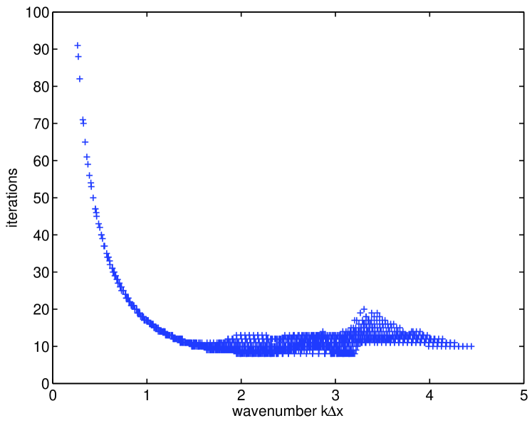
Figure 1: The number of iterations needed to reduce the error by two orders of magnitude as a function of the norm of the wave vector $k=\sqrt{k_{x}^{2}+k_{y}^{2}}$.

As we already anticipated the convergence rate for the long and the short wavelengths show the same behavior as in the one-dimensional case.

To accelerate the convergence of the long wavelengths, this iteration is applied as a smoothing function for the nonlinear multigrid scheme [17]. Using V-cycles and two pre– and post–smoothings in the multigrid scheme one achieves convergence already after two to three cycles.

5 GEM Reconnection

To verify the new iteration scheme, we choose a standard reconnection problem. A similar setup is used as in GEM reconnection challenge [7]. It is based on a perturbed Harris sheet. A schematic plot and the computational domain are shown in Fig. 2.

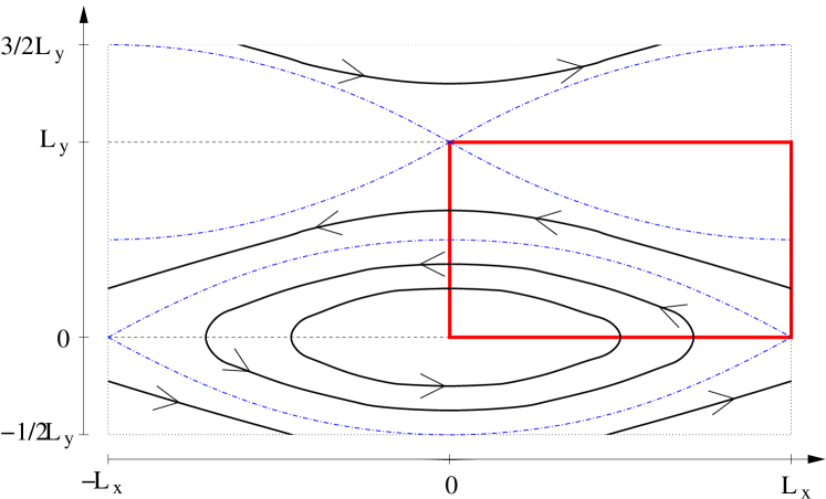
Figure 2: The GEM reconnection setup. The black lines indicate the magnetic field, the blue ones the seperatrices and the red box is our computational domain.

The numerical parameter are chosen to: $L_{x}=2L_{y}=5d_{i}$ and $N_{x}=2N_{y}=256$. Symmetric or antisymmetric boundary conditions are applied for all quantities and the initial conditions, including the perturbation, are equal to the one in the GEM reconnection challenge [7].

We solve the full Hall-MHD equations explicitly except for the Hall part of the induction equation. This splits the induction equation into the resistive MHD part (22) and the part including only the Hall term (23)

$$\partial_{t}\vec{B}_{\footnotesize\mbox{MHD}} =\nabla\times\left(\vec{v}\times\vec{B}\right)+\eta\Delta\vec{B}$$ (22)

$$\partial_{t}\vec{B}_{\footnotesize\mbox{Hall}} =-\nabla\times\left(\frac{d_{i}\vec{j}\times\vec{B}}{\rho}\right)$$ (23)

$$\partial_{t}\vec{B} =\partial_{t}\vec{B}_{\footnotesize\mbox{MHD}}+\partial_{t}\vec{B}_{\footnotesize\mbox{Hall}}\;.$$ (24)

The time stepping was performed with a standard second order Runge-Kutta method.

The maximum time step for the semi–implicit simulations is given by the linear Alfvén wave dispersion relation $\omega=v_{A}k$. There is no possibility to use larger time steps than these, because the Alfvén waves must be well resolved.

To compare the results obtained with the fully explicit simulation and with our semi–implicit treatment of the Hall term, we choose as a physically relevant measure the reconnected flux $\psi$ given in our setup by

$$\psi=\int^{L_{x}}_{0}B_{y}\ dx.$$ (25)

Four different simulation runs have been done, an explicit one, used as the reference run, and three semi–implicit ones. The time steps and corresponding CFL numbers are shown in Table 1.

	$\Delta t\cdot 10^{-3}$	CFL number	$\frac{\Delta t_{imp}}{\Delta t_{exp}}$
explicit	0.2	0.2	1
semi–implicit	2.0	2	10
semi–implicit	4.0	4	20
semi–implicit	8.2	8.2	41

Table 1: Time steps chosen for the simulations. The CFL number is based on the whistler wave dispersion relation.

Fig. 3 shows the developed structure of the $z$-component of the electric current density $\vec{j}=\nabla\times\vec{B}$ at time $t=12$ obtained from a semi–implicit simulation.

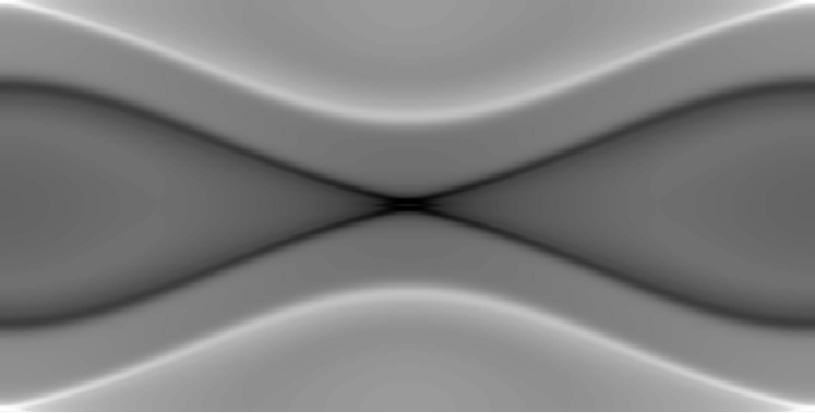
Figure 3: The $z$-component of the electric current density at $t=12$.

The corresponding reconnected flux (Fig. 4) obtained from the explicit reference simulation and the semi–implicit runs show that the the semi–implicit simulations result in nearly identical reconnection rates and that, by reducing the time step, they converge to the values obtained from the explicit simulation.

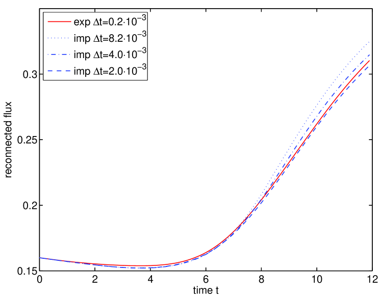
Figure 4: The temporal evolution of the reconnected flux for different time steps and schemes.

6 Summary

We presented a semi–implicit iterative method for solving the Hall part of the induction equation to overcome the time step restriction resulting from the quadratic whistler wave dispersion relation. The method utilizes a simple precondioner based on the whistler wave dispersion. The iteration scheme based on this precondioner has the two desirable features of being local and possessing strong high frequency smoothing. Therefore, this method can easily be implemented in a nonlinear multigrid solver. Due to the locality property, it is also best suited for adaptive and parallel simulations. The part of execution time of Hall term turns out to be about 7 times longer than the time needed for ideal MHD part. Using a time step 40 times larger than necessary for an explicit treatment, this results in an 80% reduction of the computation time for the GEM setup achieving nearly identical results as an expensive explicit simulation.

References

- [1] J. Dreher, D. Laveder, R. Grauer, T. Passot, P. Sulem, Formation and disruption of Alfvénic filaments in Hall-magnetohydrodynamics, Phys. Plasmas 12 (2005) 052319.
- [2] J. Dreher, V. Ruban, R. Grauer, Axisymmetric flows in Hall-MHD: A tendency towards finite-time singularity formation, Physica Scripta 72 (2005) 450.
- [3] R. F. Lottermoser, M. Scholer, Undriven magnetic reconnection in magnetohydrodynamics and Hall magnetohydrodynamics, J. Geophys. Res. 102 (1997) 4875.
- [4] M. Shay, J. Drake, The role of electron dissipation on the rate of collisionless magnetic reconnection, Geophys. Res. Lett. 25 (1998) 3759.
- [5] J. Büchner, J.-P. Kuska, Sausage mode instability of thin current sheets as a cause of magnetospheric substorms, Ann. Geophys. 17 (1999) 64.
- [6] R. Horiuchi, T. Sato, Three-dimensional particle simulation of plasma instability and collisionless reconnection in a current sheet, Phys. Plasmas 6 (1999) 4565.
- [7] J. Birn, J. Drake, M. Shay, B. Rogers, R. Denton, M. Hesse, M. Kuznetsova, Z. Ma, A. Bhattacharjee, A. Otto, P. Pritchett, Geospace environmental modeling (GEM) magnetic reconnection challenge, J. Geophys. Res. 106 (2001) 3715–3720.
- [8] P. Ricci, G. Lapenta, J. U. Brackbill, GEM reconnection challenge: Implicit kinetic simulations with the physical mass ratio, Geophys. Res. Lett. 29 (2002) 2088.
- [9] H. Schmitz, R. Grauer, Kinetic Vlasov simulations of collisionless magnetic reconnection, Phys. Plasmas 13 (2006) 092309.
- [10] D. Harned, Z. Mikić, Accurate semi-implicit treatment of the Hall effect in magnetohydrodynamic computations, J. Comp. Phys 83 (1989) 1–15.
- [11] L. Chacón, D. Knoll, A 2d high- Hall MHD implicit nonlinear solver, J. Comp. Phys 188 (2003) 573–592.
- [12] M. Berger, P. Collela, Local adaptive mesh refinement for shock hydrodynamics, J. Comp. Phys 82 (1989) 64.
- [13] B. Fryxell, K. Olsen, F. T. P. Ricker, M. Zingale, P. M. D.Q. Lamb, H. T. R. Rosner, J.W. Truran, FLASH: An adaptive mesh hydrodynamics code for modelling astrophysical thermonuclear flashes, Astrophys. J. 131 (2000) 273.
- [14] J. Dreher, R. Grauer, Racoon: A parallel mesh-adaptive framework for hyperbolic conservation laws, Parallel Computing 31 (2005) 913–932.
- [15] R. Teyssier, S. Fromang, E. Dormy, Kinematic dynamos using constrained transport with high order Godunov schemes and adaptive mesh refinement, J. Comp. Phys 218 (2006) 44–67.
- [16] C. T. Kelley, Iterative Methods for Linear and Nonlinear Equations, SIAM, 1995.
- [17] W. L. Briggs, A Multigrid Tutorial, SIAM, 2000.