Binary search trees for generalized measurement

Abstract

Generalized quantum measurements (POVMs or POMs) are important for optimally extracting information for quantum communication and computation. The standard realization via the Neumark extension requires extensive resources in the form of operations in an extended Hilbert space. For an arbitrary measurement, we show how to construct a binary search tree with a depth logarithmic in the number of possible outcomes. This could be implemented experimentally by coupling the measured quantum system to a probe qubit which is measured, and then iterating.

I Introduction

A crucial element of quantum information processing (QIP) and communication is measurement of a quantum system to access its information content, hence determining optimal measurements is important. As QIP steps out from the pages of theory and into the laboratory, one has to find implementations given the usual limited resources of the real world. The most general measurement one can perform on a quantum system is given by a positive operator valued measure (POVM) helstrom which can be considered as a projective measurement on an extended Hilbert space of which the original state resides on a (proper) sub-space. Its realization via the Neumark extension neumark ; peres requires, broadly speaking, that the extended Hilbert space should have as many dimensions as there are possible outcomes of the POVM. This has been described for atoms or ions atompom1 ; atompom2 and for linear optics hillerypom , and POVMs have been realised on optically encoded quantum information huttner ; clarke1 ; clarke2 ; steinberg .

For many physical systems, however, it is difficult or impossible to find enough extra dimensions, let alone perform operations on the extended system, hence a more efficient method is desirable. Recently, a method was discovered which allows an arbitrary POVM to be performed by adding only a single extra dimension to a system, essentially checking the measurement outcomes one by one WY2006 . However, when the number of possible measurement outcomes becomes large, more time efficient measurement strategies, also carrying a minimal dimensional overhead, would be useful. It is clear that a sequence of partial conditional measurements implements a final effective POVM with many elements peres ; GP2006 . Here we show, given any POVM, how to construct a suitable binary search tree of two-outcome POVMs by coupling the original system with a single qubit . This way, a measurement with $N=2^{t}$ outcomes can be implemented in $t$ steps, resulting in a significant speedup. Existing experimental realizations could easily be adapted to this method guerlin2007 .

II Generalized Measurement

A quantum measurement is often considered to be a projection in a complete basis of the $d$-dimensional Hilbert space. However, many experimental measurements are not well described by this. More generally, we only require of a measurement that the outcome probabilities are positive and sum to one, and satisfy convex linearity over mixtures of states. This leads to the framework of generalized quantum measurements, where a measurement is represented by a set of positive operators $\{M_{j}\}_{j=1}^{N},\text{ }\langle\psi|M_{j}|\psi\rangle\geq 0\text{ }\forall|\psi\rangle$, which sum to unity, $\sum_{j}M_{j}=\mathbb{I}$. Each outcome $j$ is associated with an operator $M_{j}$, and occurs with probability $p_{j}=\text{Tr}[M_{j}\rho]$, where $\rho$ is the measured state. Hence a generalized measurement is usually called a positive operator valued measure (POVM) or probability operator measure (POM).

The Neumark extension provides a way of performing any POVM via projective measurements, albeit in an extended space. Without loss of generality, assume that each measurement operator $M_{j}$ is proportional to a one-dimensional projector $M_{j}=|\psi_{j}\rangle\langle\psi_{j}|$ where $|\psi_{j}\rangle$ is not neccessarily normalized . If $N$ is the number of outcomes and $d$ the dimension of the Hilbert space, then $N\geq d$ will hold. If we form the $d\times N$ rectangular array $(M)_{jk}=\langle k|\psi_{j}\rangle$, where $\{|k\rangle\}$ is the computational basis, then the completeness relation implies that the columns of $(M)$ are orthonormal $N$-dimensional vectors. Hence $(M)$ can be completed to an $N$-dimensional unitary matrix $U_{M}$ whose $j^{th}$ row represents a state $|\psi_{j}^{ext}\rangle$ in an $N$-dimensional extended Hilbert space. The normalized projector $|\psi_{j}^{ext}\rangle\langle\psi_{j}^{ext}|$ corresponds to outcome $j$ for the original system. This procedure corresponds to applying $U_{M}^{\dagger}$ to the extended Hilbert space in which the original system is embedded, and then making a projective measurement in the computational basis. If $N$ is large, it may be infeasible to manipulate the required extended quantum system all at once, and we will therefore look at a way to reduce the number of ancillary dimensions by making sequential measurements.

III Sequential Measurement

The $\{M_{j}\}$ are sufficient to determine the measurement probabilities, but the post-measurement state is not uniquely defined. However, for any realization we can find Kraus operators $\{m_{j}\}$, where $M_{j}=m_{j}^{\dagger}m_{j}\text{ }\forall j$, which tell us how the quantum state is affected kraus ; peres . If outcome $j$ is obtained, then the quantum state $\rho$ is transformed to $\rho_{j}=m_{j}\rho m_{j}^{\dagger}/\text{Tr}[m_{j}\rho m_{j}^{\dagger}]$. A subsequent measurement, in general depending on the outcome $j$, acts on this transformed state.

A series of measurements can be viewed as an effective single generalized measurement, the sequence of outcomes determining the cumulative measurement operator. If the sequence $j_{1},j_{2},...,j_{t}$ of outcomes have $\{M_{j_{1}}^{1},M_{j_{2}}^{2},\ldots,M_{j_{t}}^{t}\}$ and $\{m_{j_{k}}^{k}\}$ as corresponding measurement and Kraus operators, then the final effective measurement operator and Kraus operator are given by

$$M_{j_{1},j_{2},\ldots,j_{t}} = m_{j_{1},j_{2},\ldots,j_{t}}^{\dagger}m_{j_{1},j_{2},\ldots,j_{t}},$$ (1a)

$$m_{j_{1},j_{2},\ldots,j_{t}} = m_{j_{t}}^{t}m_{j_{t-1}}^{t-1}\ldots m_{j_{1}}^{1}.$$ (1b)

Here we assume that the measurement operators and the Kraus operators are $d\times d$ operators, i.e. the measurements map the system to a Hilbert space of the same dimension . Hence, a sequence of measurements requires non-destructive measurement, e.g. indirect measurement of a system by measuring a probe after it has interacted with the system.

A series of binary outcome measurements is shown in Figure 1. The simplest probe is a two-level system (qubit), giving a binary measurement, a $d$-level probe allowing a $d$-outcome measurement. A unitary operator couples the probe with the system, e.g. via a coupling Hamiltonian over a set period. This in general entangles the state of the probe with the state of the system. Measuring the probe performs an indirect measurement of the system. From the Stinespring dilation Stinespring , this effectively implements a completely positive map with Kraus operators given by $b_{j}=\langle j|U|0\rangle$, where $\{|j\rangle\}$ is the computational basis of the probe. Outcome $j$ corresponds to the measurement operator $B_{j}=b_{j}^{\dagger}b_{j}$ and the conditional post-measurement state is

$$\rho_{j}=\frac{b_{j}\rho b_{j}^{\dagger}}{\text{Tr}[b_{j}\rho b_{j}^{\dagger}]}.$$ (2)

By choosing suitable unitaries, any binary outcome POVM can be implemented at each stage.

Conditioned on the result of the first measurement, a second measurement is performed, a third, and so on (Fig. 1). This builds up a binary measurement tree with each pair of branches representing a different binary POVM, depending on the previous results. Each node represents the effective measurement operator (given by Eq. 1b) obtained at that point. Hence, after $t$ measurements, the effective POVM may have as many as $N=d^{t}$ elements at the lowest level for a $d$-level probe.

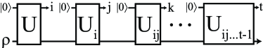
Figure 1: Sequential POVM. A probe system in the state $|0\rangle$ interacts with the measured system $\rho$ via unitaries. The probe is measured in the computational basis. Subsequent measurements, determined by $U_{x}$, are conditional upon the preceding results $i,j,k,\ldots$. The probe is reset before each measurement.

IV Binary Measurement Trees

It is easy to build up POVMs with many elements from a binary measurement tree. However, given an arbitrary POVM with elements $M_{j}$, constructing such a measurement tree which implements it is not so obvious. Here we show how it may be done.

It is instructive to look at the simplest non-trivial binary POVM tree with $t=2$ (Fig. 2). Let $B_{i}$ and $B_{ij}$ denote the binary measurement operators performed at the first and second stage, and $M_{i},M_{ij}$ denote the cumulative measurement operators. The following should hold, where $j,k=0,1$:

$$M_{j} = B_{j},$$ (3a)

$$\mathbb{I} = B_{0}+B_{1}=B_{j0}+B_{j1},$$ (3b)

$$M_{j} = M_{j0}+M_{j1},$$ (3c)

$$m_{jk} = b_{jk}m_{j}.$$ (3d)

Let us take $b_{0}=m_{0}$, $b_{1}=m_{1}$ and use the ansatz $b_{ij}=m_{ij}\tilde{b}_{i}^{-1}$ where the Moore-Penrose pseudo-inverse $\tilde{A}^{-1}$ of an operator $A$ is uniquely defined by hornjohnson

$$A\tilde{A}^{-1}A = A,$$ (4a)

$$\tilde{A}^{-1}A\tilde{A}^{-1} = \tilde{A}^{-1},$$ (4b)

$$A\tilde{A}^{-1} = (A\tilde{A}^{-1})^{\dagger},$$ (4c)

$$\tilde{A}^{-1}A = (\tilde{A}^{-1}A)^{\dagger}.$$ (4d)

We shall prove that the $b_{ij}$ so constructed correspond to POVM operators and solve the task.

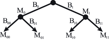
Figure 2: Four-outcome POVM. The effective measurement operators $\{M_{ij}\}$ are given by the $B$ measurements at each step. We want to determine what binary measurements $B$ are required to implement $\{M_{ij}\}$.

First, since $M_{i}$ is a positive operator, $M_{i}=\sum_{k=1}^{r}\lambda_{ik}|e_{ik}\rangle\langle e_{ik}|$, with positive eigenvalues $\lambda_{ik}$ and corresponding eigenvectors $|e_{ik}\rangle$; $r$ is the rank of $M_{i}$. The $M_{ij}$ are positive operators and $\sum_{j}M_{ij}=M_{i}$, so the null space of $M_{i}$ is contained in the null spaces of $M_{ij}$, hence $M_{ij}=\sum_{k,l=1}^{r}\phi_{ij,kl}|e_{ik}\rangle\langle e_{il}|$ for some $\phi_{ij,kl}$. Similarly, $m_{ij}=\sum_{kl=1}^{r}\varphi_{ij,kl}|e_{ik}\rangle\langle e_{il}|$ for some $\varphi_{ij,kl}$.

We can expand $b_{i}=m_{i}=\sum_{k}\sqrt{\lambda_{ik}}V_{i}|e_{ik}\rangle\langle e_{ik}|$ for some unitary $V_{i}$, similarly $\tilde{b}_{i}^{-1}=\sum_{k}1/\sqrt{\lambda_{ik}}|e_{ik}\rangle\langle e_{ik}|V_{i}^{\dagger}$. Hence, we can see that

$$(m_{ij}\tilde{b}_{i}^{-1})b_{i} = \sum_{kl=1}^{r}\varphi_{ij,kl}|e_{ik}\rangle\langle e_{il}|\sum_{s=1}^{r}\frac{1}{\sqrt{\lambda_{is}}}|e_{is}\rangle\langle e_{is}|V_{i}^{\dagger}\times$$

$$\sum_{t=1}^{r}\sqrt{\lambda_{it}}V_{i}|e_{it}\rangle\langle e_{it}|=m_{ij}.$$

In general, completeness of $\{B_{ij}\}_{j}$ requires us to modify our original ansatz by adding an extra operator,

$$b_{ij}=m_{ij}\tilde{b}_{i}^{-1}+a_{j}g_{i},$$ (5)

where $g_{i}=\sum_{j=r+1}^{d}|e_{ij}\rangle\langle e_{ij}|V_{i}^{\dagger}$ is an isometry on the null space of $b_{i}^{\dagger}$ and the coefficients satisfy $\sum_{j}|a_{j}|^{2}=1$. We have defined $g_{i}$ so that $g_{i}b_{i}=0$. With this slight modification, it is easy to show that $\sum_{k}B_{jk}=\mathbb{I}$.

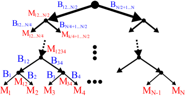
Figure 3: Binary POVM Tree. An arbitrary POVM is given by operators $M_{j}=m_{j}^{\dagger}m_{j}$. A sequence of binary outcomes with measurement operators $B_{\mu},B_{\nu},\ldots,B_{\xi}$ leads to the measurement $M_{j}=m_{j}^{\dagger}m_{j}$ where $m_{j}=b_{\xi}\ldots b_{\nu}b_{\mu}$. Half of the possible results in the branches below are eliminated at each step.

For a general POVM $\{M_{k}\}$ with $K$ elements, we first pad the set with null operators until it contains $N$ elements for $N=2^{t},t=\lceil\log_{2}K\rceil$ (Fig. 3). In a convenient change of notation, the cumulative POVM at the $j^{\text{th}}$ level consists of $2^{j}$ operators $M_{x}$ where $x$ is a sequence of $2^{t-j}$ numbers indicating which of the possible outcomes $M_{x}=\sum_{i=1}^{2^{t-j}}M_{x_{i}}$ sit in the corresponding branches below. A binary POVM $\{B_{x_{a}},B_{x_{b}}\}$ splits each node into two possible branches, each containing half of the remaining outcomes. We now determine the binary POVMs $B$ which take us from a higher to lower branch.

At the first level, $B_{12\ldots N/2}=\sum_{i=1}^{N/2}M_{i}=M_{12\ldots N/2}$ and $B_{N/2\ldots N}=\sum_{i=n/2+1}^{N}M_{i}=M_{N/2+1\ldots N}$. At the second level, from the previous section we have

$$b_{12\ldots N/4} = m_{12\ldots N/4}\tilde{b}_{12\ldots N/2}^{-1}+g_{12\ldots N/2}$$

$$b_{N/4+1\ldots N/2} = m_{N/4+1\ldots N/2}\tilde{b}_{12\ldots N/2}^{-1}+g_{12\ldots N/2}$$

$$b_{N/2+1\ldots 3N/4} = m_{N/2+1\ldots 3N/4}\tilde{b}_{N/2+1\ldots N}^{-1}+g_{N/2+1\ldots N}$$

$$b_{3N/4+1\ldots N} = m_{3N/4+1\ldots N}\tilde{b}_{N/2+1\ldots N}^{-1}+g_{N/2+1\ldots N}$$

where we have absorbed the normalization of the $g_{x}$ operators. At subsequent levels, we can express the required binary POVMs as

$$b_{x_{a}} = m_{x_{a}}\tilde{m}_{x_{a}x_{b}}^{-1}+g_{x_{a}x_{b}}$$ (6a)

$$b_{x_{b}} = m_{x_{b}}\tilde{m}_{x_{a}x_{b}}^{-1}+g_{x_{a}x_{b}}$$ (6b)

where $x_{a}x_{b}$ is the concatenation of the strings $x_{a}$ and $x_{b}$. At the last level $b_{1}=m_{1}\tilde{m}_{12}^{-1}+g_{12}$ and $b_{2}=m_{2}\tilde{m}_{12}^{-1}+g_{12}$. Note that the unitary freedom $m_{x}\rightarrow V_{j}m_{j}$ leaves the observed probabilities invariant but simply rotates the post-selected states after each measurement.

For an $N$ element POVM, we need only a probe qubit and $\lceil\log_{2}{N}\rceil$ rounds of binary measurements. Let us determine the number of operations required to implement this measurement compared to other methods. For a measurement with $N$ outcomes on a $d$-dimensional quantum system, the standard Neumark extension requires a $N\times N$ unitary transform. This can be realized with $N(N-1)/2$ operations between pairs of basis states reck , followed by a projective measurement in the $N$-dimensional space. The realization using just a single extra degree of freedom WY2006 requires a $(d+1)\times(d+1)$ unitary transform to be implemented a maximum of $N-d$ times, giving in total a maximum of $(N-d)(d+1)d/2$ operations . The binary search requires a $2d\times 2d$ transform to be implemented $\lceil\log_{2}{N}\rceil$ times, that is, $\lceil\log_{2}{N}\rceil d(2d-1)$ pairwise interactions, a significant speedup if $N$ is large.

V Example: Tetrad Measurement

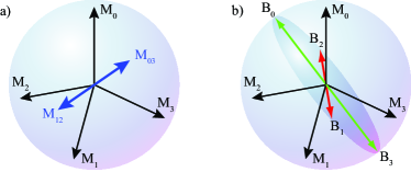
Figure 4: Tetrad POVM. a) The first binary measurement is a partial filtering with operators $\{M_{03},M_{12}\}$. b) The second (projective) measurements depend on the outcome of the first measurement. If $M_{03}$ ($M_{12}$) was obtained, then $\{B_{0},B_{3}\}$ ($\{B_{0},B_{3}\}$) is measured. The second binary measurements are projective measurements in the plane perpedicular to the directions of the first measurement and the $B_{j}$ lie in the direction of the projection of the $M_{j}$ upon this plane.

As an example of the method, consider the symmetric informationally complete POVM of a single qubit, the so-called tetrad measurement, with measurement operators $M_{j}=|\psi_{j}\rangle\langle\psi_{j}|$ given by singapore

$$|\psi_{0}\rangle = \frac{1}{\sqrt{2}}|0\rangle,$$ (7a)

$$|\psi_{1}\rangle = \frac{1}{\sqrt{6}}(|0\rangle+\sqrt{2}e^{\frac{2\pi i}{3}}|1\rangle),$$ (7b)

$$|\psi_{2}\rangle = \frac{1}{\sqrt{6}}(|0\rangle+\sqrt{2}e^{\frac{4\pi i}{3}}|1\rangle),$$ (7c)

$$|\psi_{3}\rangle = \frac{1}{\sqrt{6}}(|0\rangle+\sqrt{2}|1\rangle).$$ (7d)

Although the tetrad POVM can be performed in one projective step with the addition of just one extra qubit, it is instructive to demonstrate the binary tree approach using this example.

At the first stage, we are free to choose which two final measurement operators to group together, for instance,

$$M_{03}=B_{03}=M_{0}+M_{3}=\frac{1}{3}\left(\begin{array}[]{cc}1&\frac{1}{\sqrt{2}}\\ \frac{1}{\sqrt{2}}&2\end{array}\right),$$ (8c)

$$M_{12}=B_{12}=M_{1}+M_{2}=\frac{1}{3}\left(\begin{array}[]{cc}2&\frac{-1}{\sqrt{2}}\\ \frac{-1}{\sqrt{2}}&1\end{array}\right).$$ (8f)

We are also free to choose the Kraus operators $m_{x}=\sqrt{M_{x}}$ using the singular value decomposition. For example,

$$m_{03} = \sqrt{\lambda_{+}}|e_{+}\rangle\langle e_{+}|+\sqrt{\lambda_{-}}|e_{-}\rangle\langle e_{-}|,$$ (9a)

$$m_{12} = \sqrt{\lambda_{-}}|e_{+}\rangle\langle e_{+}|+\sqrt{\lambda_{+}}|e_{-}\rangle\langle e_{-}|,$$ (9b)

where the eigenvalues and eigenvectors are

$$\lambda_{\pm} = (1\pm\/\sqrt{3})/2,$$ (10a)

$$|e_{\pm}\rangle = (\pm\sqrt{3\pm\sqrt{3}}|0\rangle+\sqrt{3\mp\sqrt{3}}|1\rangle)/\sqrt{6}.$$ (10b)

Although $M_{03}$ and $M_{12}$ share their eigenbases, we need a full $4\times 4$ Neumark extension binary POVM so that the post-measurement state is ready for the next stage. We couple the system via $U$ to a auxiliary probe qubit prepared in the state $|0\rangle_{a}$. Then, projecting the probe onto states $|0\rangle_{a}$ and $|1\rangle_{a}$ corresponds to operations ${}_{a}\langle 0|U|0\rangle_{a}=m_{03}$ and ${}_{a}\langle 1|U|0\rangle_{a}=m_{12}$ on the system. A suitable coupling $U$ is constructed by making a $4\times 4$ Neumark extension of the two-column matrix with its first two rows given by $m_{03}$, and last two rows by $m_{12}$. In the basis $\{|e_{\pm}\rangle|j\rangle_{a}\}$, one possible $U$ is

$$U=\left(\begin{array}[]{c c c c}\sqrt{\lambda_{+}}&0&\sqrt{\lambda_{-}}&0\\ 0&\sqrt{\lambda_{-}}&0&\sqrt{\lambda_{+}}\\ \sqrt{\lambda_{-}}&0&-\sqrt{\lambda_{+}}&0\\ 0&\sqrt{\lambda_{+}}&0&-\sqrt{\lambda_{-}}\end{array}\right).$$ (11)

In this example, the positive operators $m_{jk}$ are invertible so the $b_{j}$ for the next step are easily obtained as

$$b_{0} = \sqrt{M_{0}}\sqrt{M_{03}}^{-1},\quad b_{1}=\sqrt{M_{1}}\sqrt{M_{12}}^{-1}$$ (12a)

$$b_{2} = \sqrt{M_{2}}\sqrt{M_{12}}^{-1},\quad b_{3}=\sqrt{M_{3}}\sqrt{M_{03}}^{-1},$$ (12b)

which gives

$$B_{0} = b_{0}^{\dagger}b_{0}=\frac{1}{2}\left(\begin{array}[]{cc}1+\sqrt{\frac{2}{3}}&\frac{-1}{\sqrt{3}}\\ \frac{-1}{\sqrt{3}}&1+\sqrt{\frac{2}{3}}\end{array}\right),$$ (15)

$$B_{1} = b_{1}^{\dagger}b_{1}=\frac{1}{2}\left(\begin{array}[]{cc}1&-i\\ i&1\end{array}\right),$$ (18)

$$B_{2} = b_{2}^{\dagger}b_{2}=\frac{1}{2}\left(\begin{array}[]{cc}1&i\\ -i&1\end{array}\right),$$ (21)

$$B_{3} = b_{3}^{\dagger}b_{3}=\frac{1}{2}\left(\begin{array}[]{cc}1-\sqrt{\frac{2}{3}}&\frac{1}{\sqrt{3}}\\ \frac{1}{\sqrt{3}}&1-\sqrt{\frac{2}{3}}\end{array}\right).$$ (24)

The $b_{j}$ are rank one operators but are not Hermitian. We can visualize the sequence of measurements on the Bloch ball (Fig. 4).

VI Conclusion

In conclusion, we provide a constructive proof of the universality of sequential two-outcome POVMs. We show how to construct binary measurement trees to implement any generalized measurement through a sequence of indirect binary POVMs requiring only an extra auxiliary qubit. This avoids having to manipulate extended Hilbert spaces (larger than twice the dimension of the measured system) and reduces the number of required operations when the number of outcomes becomes large. The number of steps is logarithmic in the number of measurement outcomes. The required interaction to perform binary POVMs exists in physical systems such as cavity quantum electrodynamics (CQED) guerlin2007 where the state of a field can be probed by an atom-cavity interaction and the atom measured. So far, projective measurements have been performed with a fixed interaction and measurement, but it should be possible with feed-forward and suitable control fields to implement a full POVM measurement as described here.

- (1) C. Helstrom, Quantum Detection and Estimation Theory, Academic Press, New York (1976).
- (2) M. A. Neumark, Izv. Akad. Nauk. SSSR, Ser. Mat. 4, 53277 (1940).
- (3) A. Peres, Quantum Theory: Concepts and Methods, Kluwer Academic Publishers, Dordrecht (1995).
- (4) G. Wang and M. Ying, quant-ph/0608235.
- (5) S. Franke-Arnold, E. Andersson, S. M. Barnett, and S. Stenholm, Phys. Rev. A 63, 052301 (2001).
- (6) E. Andersson, Phys. Rev. A 64, 032303 (2001).
- (7) Y. Sun, M. Hillery and J. Bergou, Phys. Rev. A 64, 022311 (2001).
- (8) B. Huttner, A. Muller, J. D. Gautier, H. Zbinden, and N. Gisin, Phys. Rev. A 54, 3783 (1996).
- (9) R. B. Clarke, A. Chefles, S. M. Barnett, and E. Riis, Phys. Rev. A 63,040305 (2001).
- (10) R. B. M. Clarke, V. M. Kendon, A. Chefles, S. M. Barnett, E. Riis, and M. Sasaki, Phys. Rev. A 64, 012303 (2001).
- (11) M. Mohseni, A. Steinberg and J. Bergou, Phys. Rev. Lett. 93, 200403 (2004).
- (12) M. G. Genoni and M. G. A. Paris, J. Phys.: Conf. Ser. 67, 012029 (2007).
- (13) C. H. Bennett, D. P. DiVincenzo, C. A. Fuchs, T. Mor, E. Rains, P. W. Shor, J. A. Smolin, and W. K. Wootters, Phys. Rev. A 59, 1070 (1999).
- (14) O. Oreshkov and T. A. Brun, Phys. Rev. Lett. 95, 110409 (2005).
- (15) S. Lloyd and L. Viola, Phys. Rev. A 65, 010101(R) (2001).
- (16) C. Guerlin, J. Bernu, S. Deléglise, C. Sayrin, S. Gleyzes, S. Kuhr, M. Brune, J.-M. Raimond and S. Haroche, Nature 448, 889 (2007).
- (17) K. Kraus, States, Effects and Operations, Springer-Verlag, Berlin (1983).
- (18) W. F. Stinespring, Proc. Amer. Math. Soc. 6, 211 (1955).
- (19) R. A. Horn and C. R. Johnson, Matrix Analysis, Cambridge University Press, Cambridge (1985).
- (20) M. Reck, A. Zeilinger, H. J. Bernstein, and P. Bertani, Phys. Rev. Lett. 73, 58 (1994).
- (21) A. Ling, K. P. Song, A. Lamas-Linares, and C. Kurtsiefer, Phys. Rev. A 74, 022309 (2006).