Fronts in randomly advected and heterogeneous media and
nonuniversality of Burgers turbulence: Theory and numerics

Abstract

A recently established mathematical equivalence—between weakly perturbed Huygens fronts (e.g., flames in weak turbulence or geometrical-optics wave fronts in slightly nonuniform media) and the inviscid limit of white-noise-driven Burgers turbulence—motivates theoretical and numerical estimates of Burgers-turbulence properties for specific types of white-in-time forcing. Existing mathematical relations between Burgers turbulence and the statistical mechanics of directed polymers, allowing use of the replica method, are exploited to obtain systematic upper bounds on the Burgers energy density, corresponding to the ground-state binding energy of the directed polymer and the speedup of the Huygens front. The results are complementary to previous studies of both Burgers turbulence and directed polymers, which have focused on universal scaling properties instead of forcing-dependent parameters. The upper-bound formula can be heuristically understood in terms of renormalization of a different kind from that previously used in combustion models, and also shows that the burning velocity of an idealized turbulent flame does not diverge with increasing Reynolds number at fixed turbulence intensity, a conclusion that applies even to strong turbulence. Numerical simulations of the one-dimensional inviscid Burgers equation using a Lagrangian finite-element method confirm that the theoretical upper bounds are sharp within about 15% for various forcing spectra (corresponding to various two-dimensional random media). These computations provide a new quantitative test of the replica method. The inferred nonuniversality (spectrum dependence) of the front speedup is of direct importance for combustion modeling.

I Introduction

In the geometrical optics of a “quenched” medium with static spatial variations in refractive index, or in the combustion of a heterogeneous solid propellant, each spatial point is characterized by a local speed $v(\mathbf{x})$ at which a wave front or flame sheet can advance normal to itself in accordance with Huygens’ principle Kerstein and Ashurst (1994). A key problem is to determine the time needed for an influence (light or combustion) to propagate from one region of space to another; Fermat’s principle asserts that the propagation effectively occurs along all possible trajectories that obey the local speed $v(\mathbf{x})$, with the first-arriving trajectory giving the desired answer.

A preliminary connection with statistical mechanics is suggested by writing the travel time for a spatial path $C$ as

$$t(C)=\int_{C}ds\,\frac{1}{v(\mathbf{x})}=\langle v^{-1}\rangle\,l(C)+\int_{C}ds\,\sigma(\mathbf{x}),$$ (1)

where $l(C)$ is the path length, $\langle v^{-1}\rangle$ is a spatial average over the medium, and $\sigma=v^{-1}-\langle v^{-1}\rangle$ is a zero-mean field. We can interpret $C$ as a material curve—a polymer string—and $t(C)$ as its potential energy, with $\langle v^{-1}\rangle$ being the constant tension and $\sigma$ an external potential. The polymer is infinitely flexible, since there is no curvature energy in Eq. (1). And the polymer is “directed” because each endpoint is confined to a different region of space. Fermat’s principle requires us to find the minimum-energy configuration (classical ground state) of this directed polymer.

So far this is just a complicated optimization problem, but it can be made more explicitly statistical in two ways. First, in many cases of interest, $\sigma$ is a homogeneous random field with specified statistics, and we are satisfied with calculating the ensemble-averaged propagation time or minimum energy (which, for a very long polymer, nearly equals the minimum energy in a single realization of $\sigma$). Second, even within a given realization of the potential, it may be convenient to consider the canonical ensemble of directed-polymer configurations at finite temperature, calculate the thermodynamic free energy, and then take the zero-temperature limit to obtain the ground-state energy. The most powerful theoretical methods arise from combining both types of ensemble.

This paper focuses on the case in which $\sigma$ is a homogeneous and isotropic (but not necessarily Gaussian) random field that is small in magnitude compared to $\langle v^{-1}\rangle$. In this weak-fluctuation limit, there is in fact a more general and useful relation between propagation and directed polymers, one that applies even to random media with time dependence and advection, such as turbulent fluids. In this paper, we focus on the quenched-medium interpretation of the analysis, but relate our approach to turbulent combustion and other applications when useful. As was recently shown Mayo and Kerstein (2007), the propagation of Huygens fronts in a broad class of weakly random $d$-dimensional media reduces to the $(d-1)$-dimensional inviscid Burgers equation with white-in-time forcing. Furthermore, the statistical properties of the inviscid Burgers dynamics are equivalent to those of viscous “Burgers turbulence” (with the same forcing) in the limit of vanishing viscosity $\nu$ Gomes et al. (2005). The white-noise-driven viscous Burgers equation, in turn, has a known relation to the canonical ensemble for a near-straight directed polymer (at a temperature proportional to $\nu$) in a $d$-dimensional static random potential that is white in one direction Bouchaud et al. (1995). This is precisely the kind of random potential commonly assumed in theoretical directed-polymer studies Mézard and Parisi (1991); Goldschmidt (1993); Blum (1994).

In Sec. II we systematically discuss some known relations among different theoretical representations of our problem, and indicate how the recent results can be linked with this framework to allow calculation of the speedup of Huygens fronts. In Sec. III we describe three rigorous “monotonicity properties” obeyed by random Huygens propagation, which provide not only checks on our later results but also further implications from them. In Sec. IV we present the replica method in a form suited to our problem, and derive explicit upper bounds on the front speedup. In Sec. V we review existing numerical simulations that provide relevant speedup values for comparison, and describe our new higher-precision simulation results. A summary and discussion are presented in Sec. VI.

II Relations among theories

II.1 KPZ, Burgers, and Huygens

The Kardar-Parisi-Zhang (KPZ) equation for interface growth Kardar et al. (1986) is well known as a unifying model for diverse phenomena. The equation can be written

$$\frac{\partial h}{\partial t}=\tfrac{1}{2}|\bm{\nabla}_{\perp}h|^{2}+\nu\nabla_{\perp}^{2}h+\eta(t,\mathbf{x}_{\perp}),$$ (2)

where $h(t,\mathbf{x}_{\perp})$ is a fluctuation in the height of an interface as a function of $d-1$ transverse dimensions and time, $\nu>0$ is a surface tension that smooths the interface, and $\eta(t,\mathbf{x}_{\perp})$ is a zero-mean external perturbation (not necessarily the white noise assumed by KPZ). Equation (2) is equivalent to the $(d-1)$-dimensional forced viscous Burgers equation

$$\frac{\partial\mathbf{w}}{\partial t}+(\mathbf{w}\cdot\bm{\nabla}_{\perp})\mathbf{w}=\nu\nabla_{\perp}^{2}\mathbf{w}-\bm{\nabla}_{\perp}\eta$$ (3)

for the velocity field $\mathbf{w}=-\bm{\nabla}_{\perp}h$, and also to the $(d-1)$-dimensional imaginary-time Schrödinger equation for the “wave function” $\exp(h/2\nu)$, with potential $-\eta$ and Planck’s constant $2\nu$. The solution of this Schrödinger equation is given by the Feynman path integral Feynman and Hibbs (1965)

$$\exp\frac{h(t,\mathbf{x}_{\perp})}{2\nu}=\int_{\mathbf{y}(t)=\mathbf{x}_{\perp}}\mathcal{D}\mathbf{y}(u)\,\exp\biggl{(}\frac{h\bm{(}0,\mathbf{y}(0)\bm{)}}{2\nu}\\ -\frac{1}{2\nu}\int_{0}^{t}du\,[\tfrac{1}{2}|\mathbf{y}^{\prime}(u)|^{2}-\eta\bm{(}u,\mathbf{y}(u)\bm{)}]\biggr{)}.$$ (4)

The simplest connection between these ideas and Huygens propagation is to assume a quenched medium with weak refractive-index fluctuations given by a smooth function $\sigma(x_{\parallel},\mathbf{x}_{\perp})$, and to write the position of a nearly flat front as the unperturbed position plus a small displacement:

$$x_{\parallel}(t,\mathbf{x}_{\perp})=t+h(t,\mathbf{x}_{\perp}),$$ (5)

in units where $\langle v^{-1}\rangle=1$. We can approximate the incremental speed $\eta(t,\mathbf{x}_{\perp})$ in Eq. (2) as the negative of the index fluctuation at the unperturbed location, i.e., $\eta(t,\mathbf{x}_{\perp})\simeq-\sigma(t,\mathbf{x}_{\perp})$. Equation (2) then governs the dynamics of $h$, with the nonlinear term describing the leading-order effect of tilted propagation, and the Laplacian term smoothing the cusps (or Burgers shocks) that would otherwise develop. (We work to leading order in the fluctuation $\sigma$ and the tilt $\bm{\nabla}_{\perp}h$, neglecting their higher-order and joint effects.) The parameter $\nu$, which corresponds to the Markstein length in premixed flamelet combustion Williams (1985), contributes a stabilizing dependence of front speed on local curvature, with concave regions propagating faster than convex regions. Pure Huygens propagation is obtained as a “viscosity solution” in the $\nu\to 0$ limit Crandall and Lions (1983); Sethian (1985).

A useful alternative description is based on a field $T_{0}(x_{\parallel},\mathbf{x}_{\perp})$ giving the time at which the front reaches a given point. From Eq. (5), we see that to leading order

$$T_{0}(x_{\parallel},\mathbf{x}_{\perp})=x_{\parallel}-h(x_{\parallel},\mathbf{x}_{\perp}).$$ (6)

Thus, in the weak-fluctuation framework, we are free to write $x_{\parallel}$ in place of $t$ as an independent variable and interpret $-h$ as the time deviation. With this perspective, the path integral (4) is, upon suitable normalization, the canonical partition function for the simple “Fermat’s principle” directed polymer described in the Introduction. With weak fluctuations, only paths that are nearly aligned with the $x_{\parallel}$-direction are competitive in travel time (energy). Such a path, described by a function $\mathbf{y}(u)$ so that $\mathbf{x}_{\perp}=\mathbf{y}(x_{\parallel})$, has arc-length element $ds=du\,[1+\tfrac{1}{2}|\mathbf{y}^{\prime}(u)|^{2}]$ and travel time

$$\begin{split}t\bm{(}\mathbf{y}(u)\bm{)}&=\int ds\,[1+\sigma\bm{(}u,\mathbf{y}(u)\bm{)}]\\ &=\int du\,[1+\tfrac{1}{2}|\mathbf{y}^{\prime}(u)|^{2}+\sigma\bm{(}u,\mathbf{y}(u)\bm{)}].\end{split}$$ (7)

Then, assuming a flat initial front with $h=0$, Eq. (4) asserts that

$$\exp\frac{-T_{0}(x_{\parallel},\mathbf{x}_{\perp})}{2\nu} =\exp\frac{-x_{\parallel}}{2\nu}\times\int_{\mathbf{y}(x_{\parallel})=\mathbf{x}_{\perp}}\mathcal{D}\mathbf{y}(u)\,\exp\biggl{(}-\frac{1}{2\nu}\int_{0}^{x_{\parallel}}du\,[\tfrac{1}{2}|\mathbf{y}^{\prime}(u)|^{2}+\sigma\bm{(}u,\mathbf{y}(u)\bm{)}]\biggr{)}$$

$$=\int_{\mathbf{y}(x_{\parallel})=\mathbf{x}_{\perp}}\mathcal{D}\mathbf{y}(u)\,\exp\frac{-t\bm{(}\mathbf{y}(u)\bm{)}}{2\nu}.$$ (8)

With the travel time as the energy, the right-hand side is the partition function at temperature $2\nu$ for a polymer with one end constrained to the initial front and the other end fixed at $(x_{\parallel},\mathbf{x}_{\perp})$. Consequently, $T_{0}(x_{\parallel},\mathbf{x}_{\perp})$ is the free energy of this polymer. As expected, Eq. (8) indicates that $T_{0}$ approaches the absolute minimum travel time (ground-state energy) in the Huygens-propagation limit $\nu\to 0$.

If $\sigma$ is a homogeneous random field, we expect the free energy $T_{0}$ to scale linearly with the longitudinal extent $x_{\parallel}$ of the polymer in the thermodynamic limit $x_{\parallel}\to\infty$. Since the ground-state energy in the absence of fluctuations would be just $x_{\parallel}$, we define the binding energy per unit length as

$$\Delta=\lim_{x_{\parallel}\to\infty}\left(1-\frac{T_{0}(x_{\parallel},\mathbf{x}_{\perp})}{x_{\parallel}}\right)=\lim_{x_{\parallel}\to\infty}\frac{h(x_{\parallel},\mathbf{x}_{\perp})}{x_{\parallel}}>0,$$ (9)

which is independent of $\mathbf{x}_{\perp}$ by homogeneity, and is positive because the nonlinear term in Eq. (2) makes $h$ increase on average. This nonlinear term equals $\tfrac{1}{2}w^{2}$, and so $\Delta$ can also be described as the steady-state energy density of the Burgers fluid. [The other two terms on the right-hand side of Eq. (2) average to zero because $h$ is statistically homogeneous in $\mathbf{x}_{\perp}$ and $\eta$ is a centered perturbation.] The effect of the weak fluctuations $\sigma$, whose rms value we denote by $\epsilon\ll 1$, is to renormalize the overall front speed upward to $v_{*}=\lim_{x_{\parallel}\to\infty}x_{\parallel}/T_{0}=1+\Delta$. Our analysis applies to the asymptotic limit $\epsilon\to 0$ and is expected to be accurate when the dimensionless parameter $\epsilon$ is small; previous numerical work Roth et al. (1993) discussed in Sec. V.1 indicates that the asymptotic scaling holds within a few percent for $\epsilon\leq 0.1$.

II.2 White-noise reduction

For media of a given structure, with fluctuations related by overall rescaling, it is clear that $\Delta\to 0$ as $\epsilon\to 0$; but the form of this dependence is subtle. If $\nu$ is fixed, then for sufficiently small $\epsilon$, Eq. (2) can be linearized; the lowest-order solution for $h$ is proportional to $\epsilon$ and thus the nonlinear term (producing the secular growth of $h$ measured by $\Delta$) is proportional to $\epsilon^{2}$. This is the weak-perturbation scenario normally associated with the KPZ equation, corresponding to a laminar solution of the viscous Burgers equation (3). On the other hand, if we take $\nu\to 0$ at finite $\epsilon$ to obtain Huygens propagation, and only then take $\epsilon\to 0$, the linearization is invalid (because the Burgers flow is fully turbulent) and the scaling of $\Delta$ with $\epsilon$ is not immediately obvious. Subject to mild conditions on the medium structure, we have shown mathematically Mayo and Kerstein (2007) that $\Delta\propto\epsilon^{4/3}$ in this regime, confirming a previous conjecture Kerstein and Ashurst (1992). Here we provide a somewhat more physical argument based on dimensional analysis.

Let us denote by $\alpha_{\parallel}$ and $\alpha_{\perp}$ some measures of the longitudinal and lateral correlation lengths of $\sigma$, and consider the behavior of the inviscid Burgers equation upon varying these quantities and $\epsilon$, while keeping fixed all other details of the statistics of $\sigma$. We can perform dimensional analysis on the KPZ equation (2), with $\eta=-\sigma$ and $\nu=0$, by assigning the conventional dimensions from the Burgers-fluid interpretation:

$$[w]=[\nabla_{\perp}h]=\mathsf{L}\mathsf{T}^{-1},\quad[h]=\mathsf{L}^{2}\mathsf{T}^{-1},\quad[\alpha_{\parallel}]=\mathsf{T},$$

$$[\alpha_{\perp}]=\mathsf{L},\quad[\eta]=[\epsilon]=\mathsf{L}^{2}\mathsf{T}^{-2},\quad[\Delta]=\mathsf{L}^{2}\mathsf{T}^{-2}.$$ (10)

(These dimensions are unusual from the viewpoint of propagation because the longitudinal and lateral directions are treated differently.) The most general dimensionless combination of input parameters is a function of $q=\alpha_{\parallel}^{2}\alpha_{\perp}^{-2}\epsilon$. Accordingly,

$$\Delta=(\alpha_{\parallel}\alpha_{\perp}^{-1}\epsilon^{2})^{2/3}\,Q(q),$$ (11)

where we have taken advantage of the freedom to choose any combination of parameters with the dimensions of $\Delta$ to multiply $Q(q)$. (We could equally well have chosen $\epsilon$ or $\alpha_{\parallel}^{-2}\alpha_{\perp}^{2}$.)

The reason for our choice is that if we take $\alpha_{\parallel}\to 0$ while scaling $\epsilon\propto\alpha_{\parallel}^{-1/2}$, so that $\sigma$ becomes white noise in the longitudinal (time) direction, then the coefficient of $Q(q)$ is unaffected. Assuming that the inviscid Burgers equation is well behaved with white-in-time forcing, so that $\Delta$ remains finite, we can partially constrain the function $Q$. The fact that $\epsilon\to\infty$ as $\alpha_{\parallel}\to 0$ is of no concern here, because the sole formally dimensionless measure of the strength of $\epsilon$ is $q$, which is approaching zero. We conclude that $Q(q)$ has a finite limit as $q\to 0$. Now, keeping the correlation lengths fixed but taking $\epsilon\to 0$ (which also gives $q\to 0$), we see that $\Delta\propto\epsilon^{4/3}$.

Our mathematical analysis Mayo and Kerstein (2007) demonstrated this result more seamlessly, starting from the exact equations of Huygens propagation (rather than from the KPZ equation), extracting a factor $\epsilon^{4/3}$ by a rescaling of variables, and directly obtaining the white-noise-driven inviscid Burgers equation as $\epsilon\to 0$. (To make the argument used in this paper more complete, in Appendix A we provide a mathematical justification for starting from the KPZ equation.) Furthermore, we showed that the effect of an advecting velocity field $\mathbf{u}$ of order $\epsilon$—along with possible time dependence of $\sigma$ and $\mathbf{u}$ on a natural timescale of order $\epsilon^{-1}$—is given as $\epsilon\to 0$ by simply adding $-u_{\parallel}$ to $\sigma$ and considering the medium as quenched at the initial time. That is, both the component $\mathbf{u}_{\perp}$ and the time dependence of the medium become irrelevant.

If we reintroduce the viscosity (Markstein length) $\nu$, with conventional dimensions $\mathsf{L}^{2}\mathsf{T}^{-1}$, there is a new dimensionless parameter that remains fixed in the white-noise limit: the Burgers-fluid Reynolds number $\mathrm{Re_{B}}\sim(\alpha_{\parallel}\alpha_{\perp}^{2}\epsilon^{2})^{1/3}\nu^{-1}$. To maintain Huygens propagation (corresponding to very large $\mathrm{Re_{B}}$) as $\epsilon\to 0$, we must decrease $\nu$ at least as fast as $\epsilon^{2/3}$. In our previous analysis, we cited mathematical results Iturriaga and Khanin (2003); Gomes et al. (2005) establishing that the white-noise-driven steady state of the inviscid Burgers equation exists, and is approached by that of the viscous Burgers equation as $\mathrm{Re_{B}}\to\infty$. Thus there is no subtlety with interchange of the limits $\epsilon\to 0$ and $\mathrm{Re_{B}}\to\infty$, as there was with $\epsilon\to 0$ and $\nu\to 0$ in Eq. (2). Previously Mayo and Kerstein (2007) we denoted by $\nu$ what we here call $\nu\epsilon^{-2/3}\propto\mathrm{Re_{B}^{-1}}$. Let us emphasize that $\mathrm{Re_{B}}$ is distinct from the hydrodynamic Reynolds number $\mathrm{Re_{NS}}$ for weak advection by a turbulent Navier-Stokes flow. In such a flow, we have $\alpha_{\parallel}\sim\alpha_{\perp}\sim L$ and $\mathrm{Re_{NS}}\sim\epsilon L\nu_{\mathrm{NS}}^{-1}$ (where we have now returned to units in which $\langle v^{-1}\rangle=1$, so that $\mathsf{L}=\mathsf{T}$ and $\epsilon$ is dimensionless). Assuming near-equality between the flame parameter $\nu$ (arising from thermal diffusivity) and the hydrodynamic viscosity $\nu_{\mathrm{NS}}$, as is valid for gaseous combustion, we have $\mathrm{Re_{B}}\sim\epsilon^{2/3}L\nu_{\mathrm{NS}}^{-1}\gg\mathrm{Re_{NS}}$ for $\epsilon\ll 1$. Thus the Burgers turbulence is more fully developed than the hydrodynamic turbulence, and the Huygens limit $\mathrm{Re_{B}}\to\infty$ is not incompatible with the physics of gaseous flames.

The quantitative implications of the white-noise reduction follow from Eq. (11). We consider altering a given physical field $\sigma$ (rms value $\epsilon\ll 1$) by multiplying the correlation length $\alpha_{\parallel}$ by $\epsilon^{2/3}$ (compressing in the longitudinal direction) and multiplying $\sigma$ everywhere by $\epsilon^{-4/3}$. The new field then has an rms value $\bar{\epsilon}=\epsilon^{-1/3}$. The parameter $q$ for the new field is unchanged from the original, and so $\Delta$ is multiplied by $\epsilon^{-4/3}$, based on the coefficient of $Q(q)$. Thus we have removed the $\epsilon^{4/3}$ dependence, and the new $\Delta$ is the prefactor. In the $\epsilon\to 0$ limit, the spectrum of the noise $\eta(x_{\parallel},\mathbf{x}_{\perp})=-\epsilon^{-4/3}\sigma(\epsilon^{-2/3}x_{\parallel},\mathbf{x}_{\perp})$, obtained by altering the original field $\sigma$ as described, becomes

$$\begin{split}D(k_{\parallel},\mathbf{k}_{\perp})&=\int dx_{\parallel}\,d^{d-1}\mathbf{x}_{\perp}\exp(-ik_{\parallel}x_{\parallel}-i\mathbf{k}_{\perp}\cdot\mathbf{x}_{\perp})\,\epsilon^{-8/3}\langle\sigma(0,\mathbf{0})\,\sigma(\epsilon^{-2/3}x_{\parallel},\mathbf{x}_{\perp})\rangle\\ &=\int dx_{\parallel}\,d^{d-1}\mathbf{x}_{\perp}\exp(-i\mathbf{k}_{\perp}\cdot\mathbf{x}_{\perp})\,\epsilon^{-2}\langle\sigma(0,\mathbf{0})\,\sigma(x_{\parallel},\mathbf{x}_{\perp})\rangle.\end{split}$$ (12)

Here we have observed that the $-ik_{\parallel}x_{\parallel}$ term is negligible because the correlation function with the argument $\epsilon^{-2/3}x_{\parallel}$ vanishes as $\epsilon\to 0$ for all nonzero $x_{\parallel}$, and we have then rescaled the integration variable $x_{\parallel}$. The spectrum is white in the longitudinal direction because there is no dependence on $k_{\parallel}$. The $\epsilon^{-2}$ factor simply normalizes the original $\sigma$ correlation function to unit variance.

Thus the desired prefactor of $\epsilon^{4/3}$ in the Huygens-front speedup is the value of $\Delta$ obtained using the path integral (4) in the $\nu\to 0$ limit, with the spectrum (12) for $\eta$. In other words, the prefactor is the ground-state binding energy per unit length for the “directed polymer” with energy

$$H=\int du\,[\tfrac{1}{2}|\mathbf{y}^{\prime}(u)|^{2}-\eta\bm{(}u,\mathbf{y}(u)\bm{)}].$$ (13)

(The ground-state energy would be zero in the absence of fluctuations, and so the binding energy is simply the negative of the free energy.) Although this is the system most commonly referred to as a directed polymer in a random potential, we observe that the white noise $\eta$ is in no sense small, and thus $\tfrac{1}{2}|\mathbf{y}^{\prime}(u)|^{2}$ is not an accurate approximation to an incremental arc length. The energy (13) is to be considered on its own terms, separate from the original intuition about a flexible string with tension. In particular, to use a supposedly more accurate square-root expression for arc length in Eq. (13) would be incorrect for our purposes. Remarkably, the idealizations conventionally adopted to render the physical directed polymer more tractable (quadratic expansion of arc length, white-noise potential) are precisely justified in the problem of weakly perturbed Huygens propagation.

III Monotonicity properties

III.1 Dependence on perturbation spectrum

It is intuitively reasonable that a more vigorous forcing of the Burgers equation should result in a higher steady-state energy density, and correspondingly that a random medium with greater fluctuations should result in faster propagation. More precisely, let us consider the $\nu\to 0$ limit of the path integral (8) for two different homogeneous weakly random media, labeled 1 and 2, and assume that at every wave vector the spectrum of $\sigma_{1}$ is no greater than that of $\sigma_{2}$. Because the spectra of independent random fields are additive, we can obtain a field $\Sigma$ with the same spectrum as $\sigma_{2}$ by defining

$$\Sigma=\sigma_{1}+\rho,$$ (14)

where $\rho$ is a zero-mean Gaussian random field (independent of $\sigma_{1}$) with an everywhere nonnegative spectrum given by subtraction. According to Eq. (12), as $\epsilon\to 0$, the speedup is governed entirely by the spectrum (or equivalently the two-point correlation function) of the medium fluctuations, and so $\Sigma$ gives the same speedup as $\sigma_{2}$.

Now we observe that the fastest path from the initial front to a given point in the field $\sigma_{1}$, which we denote $\mathbf{y}_{1}(u)$ (with travel time $t_{1}$), can be considered as a possible path in the field $\Sigma$. There, its travel time is different by an amount

$$I=\int_{0}^{x_{\parallel}}du\,\rho\bm{(}u,\mathbf{y}_{1}(u)\bm{)}.$$ (15)

The fastest path in the field $\Sigma$ must have a travel time no greater than $t_{1}+I$. The ensemble average over $\Sigma$ can then be performed in two steps, thanks to the statistical independence of $\rho$ and $\sigma_{1}$. First, upon averaging over $\rho$ for a given realization of $\sigma_{1}$, the mean of $I$ is zero and so the “partial average” first-arrival time for $\Sigma$ is no greater than $t_{1}$. Second, upon averaging over $\sigma_{1}$, the mean of $t_{1}$ is (obviously) the average first-arrival time for $\sigma_{1}$. Consequently, the “complete average” first-arrival time for $\Sigma$ (or $\sigma_{2}$) is no greater, and the speedup no smaller, than for $\sigma_{1}$.

This monotonicity property does not immediately relate the prefactors $\Delta$ of $\epsilon^{4/3}$ for different media, because two different spectra with the same total power $\epsilon^{2}$ cannot obey the assumed inequality. But relations can be obtained by considering media with $\epsilon$ differing as little as possible such that one spectrum is bounded by the other, and then correcting the result with the known $\epsilon^{4/3}$ scaling. The necessary discrepancy in $\epsilon$ (which weakens the prefactor relation) can be reduced by performing an optimally chosen spatial rescaling of one of the media, which does not affect its Huygens-front speedup.

Table 1: Correlation functions and normalized spectra of example two-dimensional random media (all homogeneous and isotropic).

Medium	$\langle\sigma(\mathbf{0})\,\sigma(\mathbf{r})\rangle$	$D(k)$
Gaussian (G)	$\epsilon^{2}\exp(-r^{2}/a^{2})$	$\pi a^{2}\exp(-\tfrac{1}{4}a^{2}k^{2})$
Modified Gaussian (MG)	$\epsilon^{2}(1-r^{2}/a^{2})\exp(-r^{2}/a^{2})$	$\tfrac{1}{4}\pi a^{4}k^{2}\exp(-\tfrac{1}{4}a^{2}k^{2})$
Exponential (E)	$\epsilon^{2}\exp(-r/a)$	$2\pi a^{2}(1+a^{2}k^{2})^{-3/2}$
Modified exponential (ME)	$\epsilon^{2}(1-\tfrac{1}{6}r^{2}/a^{2})\exp(-r/a)$	$\pi a^{4}k^{2}(7+2a^{2}k^{2})(1+a^{2}k^{2})^{-7/2}$

Table 2: Upper bounds (UB) on relative speedup from spectral monotonicity.

Medium 1	Medium 2	$\epsilon_{1}/\epsilon_{2}$	$a_{1}/a_{2}$	UB on $\Delta_{1}/\Delta_{2}$
G	E	0.723	1.414	1.541
MG	E	0.596	2.000	1.993
MG	ME	0.659	1.944	1.743
ME	E	0.904	1.029	1.144

Table 1 lists the correlation functions and spectra of four homogeneous isotropic random media in $d=2$ dimensions, which we will use as examples throughout this paper. Each medium is parametrized by the rms fluctuation $\epsilon$ and a length scale $a$. We note that the white-noise spectrum (12) is just the $d$-dimensional Fourier transform of the normalized correlation function at the wave vector $\mathbf{k}=(0,\mathbf{k}_{\perp})$. For isotropic media, this is a function $D(|\mathbf{k}_{\perp}|)$ of exactly the same form as the Fourier transform $D(k)$ at a general wave vector. The unnormalized spectrum to be used with the monotonicity property is $\epsilon^{2}\,D(k)$. Table 2 gives the results of numerically optimizing the relations between pairs of spectra to constrain the speedup prefactors $\Delta$. The omitted pairs are not useful because one spectrum dominates as $k\to 0$ and the other as $k\to\infty$.

III.2 Dependence on spatial dimension

A second monotonicity property applies when a given medium can be viewed as a “slice” through a higher-dimensional medium $M$, i.e., as the restriction of the field $\sigma$ to a (hyper)plane perpendicular to the initial front in $M$. All paths in the slice are also paths in $M$ with the same travel time, and the longitudinal coordinate $x_{\parallel}$ is the same in both media. It follows that the first-arrival time in $M$ is no greater, and the speedup no smaller, than in the slice.

For homogeneous isotropic random media, the two-point correlation function of $\sigma$ in the slice is exactly the same function of distance as in $M$. Because of the difference in dimensionality, however, its Fourier transform (i.e., the spectrum) is generally different. Of course, a correlation function is realizable only if the associated spectrum is nonnegative. We see that if a given function of distance is a realizable correlation function in $M$, it is automatically realizable in lower dimensions, and thus the spectrum (although different) remains nonnegative. But in higher dimensions, the spectrum may develop negative values and the correlation function may no longer be realizable.

The most powerful application of this monotonicity property is to a correlation function that is realizable in all dimensions, such as the Gaussian, whose Fourier transform is always another Gaussian function. In this case, the speedup prefactor must be a nondecreasing function of $d$ for all $d\geq 2$.

III.3 Dependence on laminar flame speed

The special case of Huygens propagation with advection by a random velocity field, but with a fixed front-advancement speed in the local comoving frame, is widely studied as a model of turbulent premixed combustion Williams (1985); Mayo and Kerstein (2007). There, the fixed local speed is called the laminar flame speed $u_{L}$, and the overall statistically steady propagation rate is called the turbulent burning velocity $u_{T}$. An important question in combustion modeling is the dependence of $u_{T}$ on $u_{L}$ and on the statistics of the advecting flow field (such as rms velocity $u^{\prime}$), assumed for simplicity to be given in advance rather than dynamically affected by the flame. We have shown Mayo and Kerstein (2007) that for $u^{\prime}/u_{L}\ll 1$ (weak turbulence), this idealized combustion problem is equivalent to weakly random Huygens propagation in a particular quenched medium determined by the flow statistics (specifically, the two-point spatial correlation function). Thus the methods of this paper, phrased for convenience in terms of quenched media, apply also to flames in weak turbulence.

Moreover, a simple monotonicity property allows limited conclusions even about the opposite limit $u^{\prime}/u_{L}\gg 1$ (strong turbulence, the more important case in practice). Namely, if all flow statistics are held fixed, $u_{T}$ must be a nondecreasing function of $u_{L}$. This holds realization by realization: If we consider two fronts (initially coincident) propagating independently in the same flow, the front with smaller $u_{L}$ can never get ahead of the other front anywhere, because at the location and time of any such overtaking, it would have to be advancing faster relative to the flow than its rival.

The connection between weak and strong turbulence is then as follows: For given flow statistics, the turbulent burning velocity $u_{T}$ is no greater for very small $u_{L}$ (a strong-turbulence problem) than for very large $u_{L}$ (a weak-turbulence problem). Numerically this relation is useless, since for very small $u_{L}$ we expect $u_{T}\sim u^{\prime}$, with a coefficient that remains unknown. We can only say that $u_{T}\leq\bar{u}_{L}$, where $\bar{u}_{L}\gg u^{\prime}$ is a laminar flame speed large enough that the corresponding turbulent burning velocity is essentially $\bar{u}_{L}$. But the relation is useful in ruling out the possibility that $u_{T}$ diverges to infinity at fixed $u^{\prime}$ as some other flow parameter is varied. For this to happen in strong turbulence ($u^{\prime}/u_{L}\gg 1$), it would also have to happen in weak turbulence ($u^{\prime}/u_{L}\ll 1$), i.e., the speedup prefactor $\Delta$ would have to diverge. This can be ruled out in a given case by a suitable upper bound on $\Delta$.

IV Replica analysis

IV.1 Overview of the replica method

Originally developed in the study of discrete statistical-mechanical systems such as spin glasses Edwards and Anderson (1975); Binder and Young (1986); den Hollander and Toninelli (2005), the replica method is a powerful tool for theoretical investigation of the thermodynamics of disordered systems. It exploits the interplay of two kinds of randomness: the external stochastic parameters that determine the energy “landscape” in which a system finds itself, and the finite-temperature thermal fluctuations of the system configuration within that landscape. Although we are here interested mainly in ground-state properties of the stochastic landscape, it is beneficial to consider a finite temperature and later take it to zero.

To describe the replica method in the context of our problem Mézard and Parisi (1991, 1992); Bouchaud et al. (1995), let us denote by $Z(\eta)$ the partition function for the directed polymer described by Eq. (13) with a particular realization of the white-noise potential $\eta(x_{\parallel},\mathbf{x}_{\perp})$. We are working with a polymer of a given longitudinal extent at a finite temperature $\tau$. The most general description of the disordered thermodynamics would consist of the probability density function (pdf) of $Z(\eta)$ resulting from the given statistics of $\eta$. This pdf would be difficult to obtain directly, but its moments can be simplified considerably.

For any positive integer $n$, we have

$$Z(\eta)^{n}=\int\mathcal{D}\{\mathbf{y}_{c}(u)\}\,\exp\biggl{(}-\frac{1}{\tau}\sum_{a=1}^{n}H\bm{(}\mathbf{y}_{a}(u)\bm{)}\biggr{)},$$ (16)

a product of independent path integrals over $n$ “replicas” of the polymer; here $\mathcal{D}\{\mathbf{y}_{c}(u)\}\equiv\prod_{c=1}^{n}\mathcal{D}\mathbf{y}_{c}(u)$. Because $H$ is linear in $\eta$, and because $\eta$ has Gaussian statistics, we can average Eq. (16) using the identity

$$\langle\exp\zeta\rangle=\exp(\tfrac{1}{2}\langle\zeta^{2}\rangle),$$ (17)

valid for any zero-mean Gaussian variable $\zeta$. We identify the Gaussian variable appearing in the exponential in Eq. (16),

$$\zeta=\frac{1}{\tau}\sum_{a=1}^{n}\int du\,\eta\bm{(}u,\mathbf{y}_{a}(u)\bm{)},$$ (18)

and compute

$$\begin{split}\langle\zeta^{2}\rangle&=\frac{1}{\tau^{2}}\sum_{a,b=1}^{n}\int du\,du^{\prime}\,\langle\eta\bm{(}u,\mathbf{y}_{a}(u)\bm{)}\,\eta\bm{(}u^{\prime},\mathbf{y}_{b}(u^{\prime})\bm{)}\rangle\\ &=\frac{1}{\tau^{2}}\sum_{a,b=1}^{n}\int du\,V\bm{(}|\mathbf{y}_{a}(u)-\mathbf{y}_{b}(u)|\bm{)}.\end{split}$$ (19)

We have used the relation $\langle\eta(u,\mathbf{y})\,\eta(u^{\prime},\mathbf{y}^{\prime})\rangle=\delta(u-u^{\prime})\,V(|\mathbf{y}-\mathbf{y}^{\prime}|)$, where

$$V(y)\equiv\int\frac{d^{d-1}\mathbf{k}_{\perp}}{(2\pi)^{d-1}}\,\exp(i\mathbf{k}_{\perp}\cdot\mathbf{y})\,D(|\mathbf{k}_{\perp}|).$$ (20)

Upon combining Eq. (17) with the part of $H$ that is independent of $\eta$, we obtain

$$\langle Z(\eta)^{n}\rangle=\int\mathcal{D}\{\mathbf{y}_{c}(u)\}\,\exp\biggl{(}-\frac{1}{\tau}\,H_{n}\bm{(}\{\mathbf{y}_{c}(u)\}\bm{)}\biggr{)},$$ (21)

which has the form of a single partition function for $n$ replicas with “energy”

$$\begin{split}H_{n}=\int du\,\biggl{(}&\tfrac{1}{2}\sum_{a=1}^{n}|\mathbf{y}^{\prime}_{a}(u)|^{2}\\ &-\frac{1}{2\tau}\sum_{a,b=1}^{n}V\bm{(}|\mathbf{y}_{a}(u)-\mathbf{y}_{b}(u)|\bm{)}\biggr{)}.\end{split}$$ (22)

This $H_{n}$, unlike $H$, contains no random potential, but the price is that we now have several interacting polymers (a different number of them for each different moment of $Z$ we wish to calculate).

Much as in Sec. II.1, the new partition function $\langle Z^{n}\rangle$ can be identified as a Feynman path integral for the $n$-particle imaginary-time Schrödinger equation, with Planck’s constant $\tau$ and with the potential $-V/2\tau$ acting on every pair of particles (including self-interaction). The potential function is now static and deterministic, unlike the time-dependent random potential $-\eta$ in the original Schrödinger equation. The wave function $\psi(\mathbf{y}_{1},\dotsc,\mathbf{y}_{n})$ is governed by the Hamiltonian operator

$$\mathcal{H}_{n}=-\tfrac{1}{2}\tau^{2}\sum_{a=1}^{n}\nabla_{a}^{2}-\frac{1}{2\tau}\sum_{a,b=1}^{n}V(|\mathbf{y}_{a}-\mathbf{y}_{b}|).$$ (23)

The thermodynamic limit of an infinitely long polymer has a simple interpretation: By evolving the imaginary-time Schrödinger equation

$$\frac{\partial\psi}{\partial x_{\parallel}}=-\frac{1}{\tau}\,\mathcal{H}_{n}\psi$$ (24)

for an infinite time, we project any initial wave function onto the quantum ground state. The path integral for $\langle Z^{n}\rangle$ over a sufficiently long time $x_{\parallel}$ is dominated by a term proportional to $\exp[-E_{g}(n)\,x_{\parallel}/\tau]$, where $E_{g}(n)$ is the ground-state energy of the $n$-particle system, because the contributions of the other (higher) energy eigenvalues are asymptotically negligible.

What we actually wish to calculate is not a moment $\langle Z^{n}\rangle$ but the averaged free energy $-\tau\langle\ln Z\rangle$. Unfortunately, $\ln Z$ cannot be expanded in a Taylor series about $Z=0$, and to make progress we must introduce a peculiar feature of the replica method. The needed average is expressed by the identity

$$\langle\ln Z\rangle=\lim_{n\to 0}\frac{\langle Z^{n}\rangle-1}{n},$$ (25)

and it is assumed that $\langle Z^{n}\rangle$, computed as above for positive integer $n$, can be analytically continued to $n$ near zero. Then the asymptotic (large $x_{\parallel}$) behavior of the averaged free energy is

$$\begin{split}{-}\tau\langle\ln Z\rangle&=-\tau\lim_{n\to 0}\frac{\exp[-E_{g}(n)\,x_{\parallel}/\tau]-1}{n}\\ &=x_{\parallel}\lim_{n\to 0}\frac{E_{g}(n)}{n},\end{split}$$ (26)

and so the polymer’s binding energy per unit length is

$$\Delta=-\lim_{n\to 0}\frac{E_{g}(n)}{n}.$$ (27)

IV.2 Variational treatment

We desire a method for estimating $E_{g}(n)$ that is demonstrably valid for any positive integer $n$ and that also (unlike, e.g., numerical solution of the $n$-particle Schrödinger equation) can be formally generalized to noninteger $n$. A very useful choice is the variational method, which is based on the observation that the expectation value $\langle\psi|\mathcal{H}_{n}|\psi\rangle$ of the $n$-particle Hamiltonian in an arbitrary quantum state $|\psi\rangle$ is an upper bound on $E_{g}(n)$. To obtain as tight a bound as possible, this expectation value is minimized over a convenient family of “trial” wave functions, in the hope that some of them are close to the true ground state.

The variational method is valid for positive integer $n$, where $\mathcal{H}_{n}$ is a Hermitian operator on a well-defined Hilbert space. The wave function associates a number with each configuration of $n$ particles in $d-1$ dimensions, but because the Hamiltonian is translation invariant, the center of mass separates and the nontrivial part of the wave function depends on $n-1$ vectors. Furthermore, the wave function is subject to one normalization constraint, $\langle\psi|\psi\rangle=1$. Thus the number of degrees of freedom in the wave function can be written

$$f=\infty^{(d-1)(n-1)}-1.$$ (28)

When $n=1$, for example, we have $f=0$ (no degrees of freedom), as expected because there is a unique translation-invariant one-particle wave function, the eigenstate of zero momentum. This variational estimate is automatically the exact ground state of the free-particle Hamiltonian $\mathcal{H}_{1}$.

For $n\to 0$, we have $f=-1$, and the replica method relies on the following nonrigorous argument: If $E_{g}(n)$ is the minimum of $\langle\psi|\mathcal{H}_{n}|\psi\rangle$ with respect to a separate variation in each degree of freedom of $|\psi\rangle$ around the true ground state, then when the degrees of freedom are themselves negative in number, any conceivable variation of $|\psi\rangle$ will result in a decrease of $\langle\psi|\mathcal{H}_{n}|\psi\rangle$. Consequently, we maximize $\langle\psi|\mathcal{H}_{n}|\psi\rangle$ among trial wave functions and thereby obtain a lower bound on $E_{g}(n)$. The results of applying this strategy to spin glasses have been verified by rigorous methods Guerra (2003); Talagrand (2006), and there is no evidence that the corresponding results for directed polymers are invalid. In fact, the numerical simulations in Sec. V provide a successful quantitative test of this application of the replica method.

In Appendix B we analyze a commonly used family of trial wave functions, parametrized by a function $z(u)$, for which $\langle\psi|\mathcal{H}_{n}|\psi\rangle$ can be expressed analytically in $n$. The result is

$$\begin{split}\langle\psi|\mathcal{H}_{n}|\psi\rangle={}&\tfrac{1}{8}\tau^{2}(d-1)n\int_{1}^{n}\frac{du}{u^{2}\,\Lambda(u)}\\ &-\frac{n}{2\tau}\left(B_{0}(0)+\int_{1}^{n}du\,B_{0}\bm{(}z(u)\bm{)}\right),\end{split}$$ (29)

where

$$\Lambda(u) =\tfrac{1}{2}u\,z(u)-\tfrac{1}{2}\int_{1}^{u}dv\,z(v),$$ (30)

$$B_{0}(z) =\int\frac{d^{d-1}\mathbf{k}_{\perp}}{(2\pi)^{d-1}}\,\exp(-\tfrac{1}{2}|\mathbf{k}_{\perp}|^{2}z)\,D(|\mathbf{k}_{\perp}|).$$ (31)

As $n\to 0$, a meaningful wave function requires $z(u)$ to be nonnegative and nonincreasing for $0<u<1$. If we define

$$\begin{split}\Gamma(\tau,z)={}&-\lim_{n\to 0}\frac{\langle\psi|\mathcal{H}_{n}|\psi\rangle}{n}\\ ={}&\tfrac{1}{8}\tau^{2}(d-1)\int_{0}^{1}\frac{du}{u^{2}\,\Lambda(u)}\\ &+\frac{1}{2\tau}\left(B_{0}(0)-\int_{0}^{1}du\,B_{0}\bm{(}z(u)\bm{)}\right),\end{split}$$ (32)

then the polymer’s binding energy per unit length at temperature $\tau$ is bounded above by $\Gamma(\tau,z)$ for any nonnegative, nonincreasing function $z(u)$. Thus the Huygens prefactor $\Delta$ obeys

$$\Delta\leq\lim_{\tau\to 0}\Gamma(\tau,z_{\tau}),$$ (33)

where we anticipate based on previous results Blum (1994) that a useful, finite bound will require a $\tau$-dependent choice of $z(u)$.

IV.3 Explicit replica bounds

The replica variational treatment has been applied in some detail to the directed-polymer problem, focusing on the case of the Gaussian medium Blum (1994). In that work, all values of temperature were considered, and the goal was a general qualitative understanding of the polymer’s behavior, rather than a calculation of its binding energy. Here, by concentrating on the binding energy in the zero-temperature limit, we are able to extend the previous results to obtain explicit bounds on $\Delta$, not only for the Gaussian medium but for arbitrary spectra. (“Gaussian” refers to a type of spectrum, defined for $d=2$ in Table 1. As discussed in Sec. II.2, a quite separate feature of Huygens propagation is the equivalence of weak isotropic perturbations, not necessarily Gaussian in pdf, to the directed polymer’s white-noise perturbations, which are automatically Gaussian in pdf and described completely by their spectrum.)

We start with a derivation of the equation for stationarity of $\Gamma(\tau,z)$ and its consequences, along the lines of the previous work Blum (1994). From Eq. (98), we compute

$$\frac{\delta\Lambda(v)}{\delta z(u)}=\tfrac{1}{2}u\,\delta(u-v)+\tfrac{1}{2}\,\theta(u-v),$$ (34)

where $\theta(x)$ equals $1$ for $x>0$ and $0$ for $x<0$, and thus

$$\begin{split}\frac{\delta\Gamma(\tau,z)}{\delta z(u)}&=-\tfrac{1}{16}\tau^{2}(d-1)\int_{0}^{1}\frac{dv}{v^{2}\,\Lambda(v)^{2}}[u\,\delta(u-v)+\theta(u-v)]-\frac{1}{2\tau}\,B_{0}^{\prime}\bm{(}z(u)\bm{)}\\ &=-\tfrac{1}{16}\tau^{2}(d-1)\left(\frac{1}{u\,\Lambda(u)^{2}}+\int_{0}^{u}\frac{dv}{v^{2}\,\Lambda(v)^{2}}\right)+\frac{1}{2\tau}\,B_{1}\bm{(}z(u)\bm{)}.\end{split}$$ (35)

We use the notation

$$\begin{split}B_{p}(z)&\equiv(-1)^{p}\,\frac{d^{p}B_{0}(z)}{dz^{p}}\\ &=\int\frac{d^{d-1}\mathbf{k}_{\perp}}{(2\pi)^{d-1}}\,(\tfrac{1}{2}|\mathbf{k}_{\perp}|^{2})^{p}\exp(-\tfrac{1}{2}|\mathbf{k}_{\perp}|^{2}z)\,D(|\mathbf{k}_{\perp}|);\end{split}$$ (36)

note that each $B_{p}(z)$ is a positive, decreasing function for $z>0$.

In the absence of constraints on $z(u)$, the variational optimum would satisfy $\delta\Gamma/\delta z=0$. Inserting Eq. (35) and differentiating with respect to $u$, we obtain

$$\tfrac{1}{8}\tau^{2}(d-1)\,\frac{\Lambda^{\prime}(u)}{u\,\Lambda(u)^{3}}-\frac{1}{2\tau}\,B_{2}\bm{(}z(u)\bm{)}\,z^{\prime}(u)=0,$$ (37)

or, using Eq. (105),

$$z^{\prime}(u)\left(\frac{\tau^{2}(d-1)}{16\,\Lambda(u)^{3}}-\frac{B_{2}\bm{(}z(u)\bm{)}}{2\tau}\right)=0.$$ (38)

Regions where $z^{\prime}(u)=0$ (for which infinitesimal variations could violate the nonincreasing constraint) still obey Eq. (38). Provided $z(u)>0$ everywhere (so that the nonnegative constraint has no local effect), Eq. (38) is a necessary condition for an optimum.

The type of solution obtained for the $d=2$ Gaussian medium Blum (1994) has the second factor in Eq. (38) equal to zero for $0<u<u_{\text{c}}$, while $z(u)=z(u_{\text{c}})$ for $u_{\text{c}}<u<1$ so that the first factor $z^{\prime}(u)$ equals zero there. Thus we have

$$\Lambda(u) =\tfrac{1}{2}\tau\left(\frac{d-1}{B_{2}\bm{(}z(u)\bm{)}}\right)^{1/3} (0<u<u_{\text{c}}),$$ (39)

$$\Lambda(u) =\tfrac{1}{2}\,z(u_{\text{c}}) (u_{\text{c}}<u<1).$$ (40)

From the assumed continuity of $z(u)$ at $u_{\text{c}}$, the continuity of $\Lambda(u)$ follows, and so

$$\tfrac{1}{2}\,z(u_{\text{c}})=\Lambda(u_{\text{c}})=\tfrac{1}{2}\tau\left(\frac{d-1}{B_{2}\bm{(}z(u_{\text{c}})\bm{)}}\right)^{1/3}.$$ (41)

As $\tau\to 0$, this gives

$$z(u_{\text{c}})=\tau\left(\frac{d-1}{B_{2}(0)}\right)^{1/3}.$$ (42)

Also, by differentiating Eq. (39), we find

$$\Lambda^{\prime}(u) =\tfrac{1}{6}\tau\,\frac{(d-1)^{1/3}}{B_{2}\bm{(}z(u)\bm{)}^{4/3}}\,B_{3}\bm{(}z(u)\bm{)}\,z^{\prime}(u) (0<u<u_{\text{c}}),$$ (43)

or, assuming $z^{\prime}(u)\neq 0$ and using Eq. (105),

$$u =\tfrac{1}{3}\tau\,\frac{(d-1)^{1/3}}{B_{2}\bm{(}z(u)\bm{)}^{4/3}}\,B_{3}\bm{(}z(u)\bm{)} (0<u<u_{\text{c}}).$$ (44)

This constitutes an implicit solution for $z(u)$. We would like to make use of this solution as far as possible for arbitrary spectra, without adopting particular forms of $B_{p}$.

Let us define

$$\mu(z)=\frac{B_{3}(z)}{B_{2}(z)^{4/3}}.$$ (45)

The simplest case occurs when $\mu(z)$ is a decreasing function for all $z>0$ and $\lim_{z\to\infty}\mu(z)=0$. Then a single-valued, decreasing function $z(u)$ for $0<u<u_{\text{c}}$ is defined by

$$u =\tfrac{1}{3}\tau(d-1)^{1/3}\,\mu(z) [z(u_{\text{c}})<z<\infty],$$ (46)

where $z(u_{\text{c}})$ is given by Eq. (42). We now attempt to substitute this trial solution into Eq. (32). Upon integration by parts, the first term of $\Gamma(\tau,z)$ becomes

$$\begin{split}\Gamma_{1}={}&\tfrac{1}{8}\tau^{2}(d-1)\left(\frac{1}{\Lambda(u_{\text{c}})}\int_{u_{\text{c}}}^{1}\frac{du}{u^{2}}+\int_{0}^{u_{\text{c}}}\frac{du}{u^{2}\,\Lambda(u)}\right)\\ ={}&\tfrac{1}{8}\tau^{2}(d-1)\\ &\times\left(\frac{1/u_{\text{c}}-1}{\Lambda(u_{\text{c}})}-\int_{0}^{u_{\text{c}}}du\,\frac{\Lambda^{\prime}(u)}{u\,\Lambda(u)^{2}}-\left.\frac{1}{u\,\Lambda(u)}\right|_{0}^{u_{\text{c}}}\right)\\ ={}&\tfrac{1}{8}\tau^{2}(d-1)\\ &\times\left(-\frac{1}{\Lambda(u_{\text{c}})}-\tfrac{1}{2}\int_{0}^{u_{\text{c}}}du\,\frac{z^{\prime}(u)}{\Lambda(u)^{2}}+\lim_{u\to 0}\frac{1}{u\,\Lambda(u)}\right).\end{split}$$ (47)

To evaluate the limit, we observe that $u\to 0$ corresponds to $z\to\infty$. If $D(k)\sim k^{q}$ as $k\to 0$, then for the total power

$$\int\frac{d^{d}\mathbf{k}}{(2\pi)^{d}}\,D(k)$$ (48)

to be finite, as required to define the parameter $\epsilon$ of the random medium, we must have $q+d>0$. The resulting behavior of $B_{p}$, from Eq. (36), is

$$B_{p}(z) \sim z^{-p-(q+d-1)/2} (z\to\infty).$$ (49)

Using Eqs. (39) and (46), we find

$$u\,\Lambda(u) \propto\frac{B_{3}(z)}{B_{2}(z)^{5/3}}\sim z^{(q+d)/3}\to\infty (z\to\infty),$$ (50)

and so the limit in Eq. (47) is zero. Furthermore, from Eq. (41), the term $\propto\tau^{2}/\Lambda(u_{\text{c}})$ in Eq. (47) scales with $\tau$ and vanishes as $\tau\to 0$. Under a change of variable to $z$, the remaining integral gives

$$\Gamma_{1}=\tfrac{1}{4}(d-1)^{1/3}\int_{z(u_{\text{c}})}^{\infty}dz\,B_{2}(z)^{2/3}.$$ (51)

The second term of $\Gamma(\tau,z)$ becomes

$$\begin{split}\Gamma_{2}=\frac{1}{2\tau}\,\biggl{(}&B_{0}(0)-B_{0}\bm{(}z(u_{\text{c}})\bm{)}\int_{u_{\text{c}}}^{1}du\\ &-\int_{0}^{u_{\text{c}}}du\,B_{0}\bm{(}z(u)\bm{)}\biggr{)}\\ =\frac{1}{2\tau}\,\biggl{(}&B_{0}(0)-(1-u_{\text{c}})\,B_{0}\bm{(}z(u_{\text{c}})\bm{)}\\ &+\int_{z(u_{\text{c}})}^{\infty}dz\,B_{0}(z)\,u^{\prime}(z)\biggr{)},\end{split}$$ (52)

where $u(z)$ is given by Eq. (46). Integration by parts then yields

$$\Gamma_{2}=\frac{1}{2\tau}\,\biggl{(}B_{0}(0)-B_{0}\bm{(}z(u_{\text{c}})\bm{)}+\int_{z(u_{\text{c}})}^{\infty}dz\,B_{1}(z)\,u(z)\biggr{)},$$ (53)

because $\lim_{z\to\infty}B_{0}(z)\,u(z)=0$. Recognizing a difference quotient, which as $\tau\to 0$ becomes a derivative $\propto B_{0}^{\prime}(0)$, we obtain

$$\begin{split}\Gamma_{2}={}&\tfrac{1}{2}\,B_{1}(0)\left(\frac{d-1}{B_{2}(0)}\right)^{1/3}\\ &+\tfrac{1}{6}(d-1)^{1/3}\int_{z(u_{\text{c}})}^{\infty}dz\,\frac{B_{1}(z)\,B_{3}(z)}{B_{2}(z)^{4/3}}.\end{split}$$ (54)

In both Eqs. (51) and (54), the lower limits of the integrals can be taken to zero by Eq. (42), since there is no remaining singular dependence on $\tau$. Also, because

$$\frac{d}{dz}\,\frac{B_{1}(z)}{B_{2}(z)^{1/3}}=-B_{2}(z)^{2/3}+\tfrac{1}{3}\,\frac{B_{1}(z)\,B_{3}(z)}{B_{2}(z)^{4/3}},$$ (55)

Eq. (54) simplifies upon a further integration by parts to

$$\begin{split}\Gamma_{2}={}&\tfrac{1}{2}(d-1)^{1/3}\int_{0}^{\infty}dz\,B_{2}(z)^{2/3}\\ &+\tfrac{1}{2}(d-1)^{1/3}\lim_{z\to\infty}\frac{B_{1}(z)}{B_{2}(z)^{1/3}}.\end{split}$$ (56)

The limit vanishes because

$$\frac{B_{1}(z)}{B_{2}(z)^{1/3}} \sim z^{-(q+d)/3}\to 0 (z\to\infty).$$ (57)

Thus we obtain the replica bound

$$\Delta\leq\Gamma_{1}+\Gamma_{2}=\tfrac{3}{4}(d-1)^{1/3}\int_{0}^{\infty}dz\,B_{2}(z)^{2/3}$$ (58)

on the prefactor of the Huygens-front speedup.

A remarkable renormalization interpretation of Eq. (58) is seen by rewriting it as

$$\Delta\leq\tfrac{3}{4}(d-1)^{1/3}\int_{0}^{\infty}\frac{dz}{z}\,[z^{3/2}\,B_{2}(z)]^{2/3}.$$ (59)

Note that

$$\begin{split}z^{3/2}\,B_{2}&(z)\\ ={}&\int\frac{d^{d-1}\mathbf{k}_{\perp}}{(2\pi)^{d-1}}\,\tfrac{1}{4}|\mathbf{k}_{\perp}|^{4}\,z^{3/2}\exp(-\tfrac{1}{2}|\mathbf{k}_{\perp}|^{2}z)\,D(|\mathbf{k}_{\perp}|)\\ ={}&\tfrac{1}{2}\pi^{1/2}\,\frac{\Gamma(\frac{1}{2}d)}{\Gamma\bm{(}\frac{1}{2}(d-1)\bm{)}}\\ &\times\int\frac{d^{d}\mathbf{k}}{(2\pi)^{d}}\,(k^{2}z)^{3/2}\exp(-\tfrac{1}{2}k^{2}z)\,D(k),\end{split}$$ (60)

where we have inserted factors to compensate increasing the integration from $d-1$ to $d$ dimensions. Because the integrand becomes small for $k\ll z^{-1/2}$ or $k\gg z^{-1/2}$, Eq. (60) represents the power contained in a finite wave-number band around $k\sim z^{-1/2}$ of width $\delta k\sim z^{-1/2}$. In Eq. (59), this spectral band power (analogous to $\epsilon^{2}$) is raised to the $\frac{2}{3}$ power (consistent with $\epsilon^{4/3}$ scaling) and then integrated over all logarithmic length scales ($dz/z$). This suggests a stepwise process in which, starting from the smallest length scales, each order-unity spectral band has the same qualitative effect as if acting alone: It renormalizes the front propagation speed, with the new effective speed (turbulent burning velocity in combustion) providing the raw input (laminar flame speed) for the next larger-length-scale band. In the weak-perturbation limit of Huygens propagation, because all these renormalization contributions are very small, they combine additively as displayed in Eq. (59). These conclusions are compared to existing concepts of front-speed renormalization in Sec. VI.

The assumptions about $\mu(z)$ stated below Eq. (45) hold for the two-dimensional Gaussian and exponential media in Table 1. As a result, bounds on their speedup prefactors can be obtained from Eq. (58):

$$\Delta_{\text{G}} \leq\frac{3^{8/3}\pi^{1/3}}{16}\simeq 1.714,$$ (61)

$$\Delta_{\text{E}} \leq 2.038.$$ (62)

For the exponential medium, due to the long spectral tail at high wave number, $B_{p}(0)$ is divergent for $p\geq 1$. Although such quantities appeared in the derivation, the exponential medium can be approached by a limiting process to make the expressions well-defined. The end result, Eq. (58), is finite and was evaluated directly by numerical integration to obtain Eq. (62).

We now consider violations of the previous assumptions about $\mu(z)$. If $\mu(z)$ is decreasing for all $z>0$ but $\lim_{z\to\infty}\mu(z)=\mu_{*}>0$, then we define $z(u)$ by Eq. (46) for $\frac{1}{3}\tau(d-1)^{1/3}\mu_{*}\equiv u_{*}<u<u_{\text{c}}$, and define $z(u)=\infty$ for $0<u<u_{*}$. It follows that $\Lambda(u)=\infty$ for $0<u<u_{*}$, and so both integrals in Eq. (32) receive nonzero contributions only from $u_{*}<u<1$, since $B_{0}(\infty)=0$. The change of variable to $z$ and the integrations by parts proceed as before, and the result (58) is unchanged.

On the other hand, if $\mu(z)$ is not an everywhere decreasing function, let $[0,z_{*}]$ be the largest interval from zero on which it is decreasing (possibly $z_{*}=0$). We define $u_{*}=\frac{1}{3}\tau(d-1)^{1/3}\,\mu(z_{*})$ and again take $z(u)=\Lambda(u)=\infty$ for $0<u<u_{*}$. Then the $z$ integrals extend only up to $z_{*}$, and several boundary terms from integration by parts no longer vanish. Specifically, we find

$$\begin{split}\Gamma_{1}={}&\tfrac{1}{8}\tau^{2}(d-1)\,\frac{1}{u_{*}\,\Lambda(u_{*})}\\ &+\tfrac{1}{4}(d-1)^{1/3}\int_{0}^{z_{*}}dz\,B_{2}(z)^{2/3},\end{split}$$ (63)

$$\begin{split}\Gamma_{2}={}&\frac{1}{2\tau}\,B_{0}(z_{*})\,u_{*}+\tfrac{1}{2}(d-1)^{1/3}\,\frac{B_{1}(z_{*})}{B_{2}(z_{*})^{1/3}}\\ &+\tfrac{1}{2}(d-1)^{1/3}\int_{0}^{z_{*}}dz\,B_{2}(z)^{2/3},\end{split}$$ (64)

and thus

$$\begin{split}\Delta\leq{}&\Gamma_{1}+\Gamma_{2}\\ ={}&(d-1)^{1/3}\,\biggl{(}\tfrac{3}{4}\,\frac{B_{2}(z_{*})^{5/3}}{B_{3}(z_{*})}+\tfrac{1}{6}\,\frac{B_{0}(z_{*})\,B_{3}(z_{*})}{B_{2}(z_{*})^{4/3}}\\ &+\tfrac{1}{2}\,\frac{B_{1}(z_{*})}{B_{2}(z_{*})^{1/3}}+\tfrac{3}{4}\int_{0}^{z_{*}}dz\,B_{2}(z)^{2/3}\biggr{)}.\end{split}$$ (65)

This bound applies to the two remaining media in Table 1. For the modified Gaussian medium, $\mu(z)$ is in fact an increasing function for $z>0$, so we take $z_{*}=0$, giving

$$\Delta_{\text{MG}}\leq\frac{359\pi^{1/3}}{2^{8/3}3^{4/3}5^{1/3}7}\simeq 1.599.$$ (66)

For the modified exponential medium, numerical evaluation shows that $\mu(z)$ is decreasing only for $0<z<z_{*}\simeq 7.492$, giving

$$\Delta_{\text{ME}}\leq 1.943.$$ (67)

The reason $\mu(z)$ ultimately increases for these media is that $D(k)\sim k^{2}$ as $k\to 0$. From Eq. (49) with $q=2$ and $d=2$, we find that $\mu(z)\sim z^{1/6}$ as $z\to\infty$. By contrast, two-dimensional media with $D(k)\sim k^{0}$ as $k\to 0$ have $\mu(z)\sim z^{-1/6}$ as $z\to\infty$.

It is possible to obtain a slightly better bound on $\Delta_{\text{MG}}$. Because $z_{*}=0$ for this medium, no real use has been made of the solution (44). The trial functions we have constructed are simply piecewise constant, of the form

$$z(u) =\infty, \Lambda(u) =\infty (0<u<u_{\text{c}}),$$ (68)

$$z(u) =z_{\text{c}}, \Lambda(u) =\tfrac{1}{2}z_{\text{c}} (u_{\text{c}}<u<1).$$ (69)

We can discard the earlier motivation and consider arbitrary permissible values of $u_{\text{c}}$ and $z_{\text{c}}$. Upon variational optimization, Eqs. (68) and (69) are known as the one-step solution because only one level of replica symmetry breaking is needed ($K=1$, $m_{1}=u_{\text{c}}$). This solution was previously discussed for the directed polymer with arbitrary perturbation spectrum Goldschmidt (1993) and will now be derived in our notation. Equation (32) becomes

$$\begin{split}\Gamma(\tau,z)={}&\tfrac{1}{8}\tau^{2}(d-1)\left(\frac{1}{u_{\text{c}}}-1\right)\frac{2}{z_{\text{c}}}\\ &+\frac{1}{2\tau}\,[B_{0}(0)-(1-u_{\text{c}})\,B_{0}(z_{\text{c}})].\end{split}$$ (70)

Stationarity with respect to $u_{\text{c}}$ and $z_{\text{c}}$ gives

$$-\tfrac{1}{4}\tau^{2}(d-1)\,\frac{1}{u_{\text{c}}^{2}z_{\text{c}}}+\frac{B_{0}(z_{\text{c}})}{2\tau} =0,$$ (71)

$$-\tfrac{1}{4}\tau^{2}(d-1)\,\left(\frac{1}{u_{\text{c}}}-1\right)\frac{1}{z_{\text{c}}}+(1-u_{\text{c}})\,\frac{B_{1}(z_{\text{c}})}{2\tau} =0.$$ (72)

As $\tau\to 0$, the solution is

$$u_{\text{c}} =\tau\left(\frac{d-1}{2}\right)^{1/3}\,\frac{B_{1}(0)^{1/3}}{B_{0}(0)^{2/3}},$$ (73)

$$z_{\text{c}} =\tau\left(\frac{d-1}{2}\right)^{1/3}\,\frac{B_{0}(0)^{1/3}}{B_{1}(0)^{2/3}},$$ (74)

and substituting into Eq. (70) shows that

$$\Delta\leq\tfrac{3}{2}\left(\frac{d-1}{2}\right)^{1/3}\,B_{0}(0)^{1/3}\,B_{1}(0)^{1/3}.$$ (75)

For the two-dimensional modified Gaussian medium, Eq. (75) gives a tighter bound than Eq. (66),

$$\Delta_{\text{MG}}\leq\frac{3^{4/3}\pi^{1/3}}{4}\simeq 1.585,$$ (76)

as expected because we have optimized over a new family that includes our previous trial solution. For the Gaussian medium, we obtain a looser bound than before ($\Delta_{\text{G}}\leq 3\pi^{1/3}/2^{4/3}\simeq 1.744$); for the exponential and modified exponential media, since $B_{1}(0)$ diverges, the one-step upper bound is infinite and uninformative.

IV.4 Implications of the replica results

We now discuss the replica results in light of the monotonicity properties of Sec. III. The finite-band-renormalization interpretation described below Eq. (58) indicates that media with broader spectra (on a logarithmic wave-number scale) should have larger bounds on $\Delta$. This is because the spectral power is more widely dispersed among bands, giving a lower amount per band before each is raised to the $\frac{2}{3}$ power, and $x^{2/3}$ decreases more slowly than $x$ as $x$ becomes small. [The limit $x\to 0$ corresponds to a spectrum $D(k)\propto k^{-d}$ with power spread equally over many orders of magnitude in wave number.] Indeed, the replica bounds on $\Delta$ are larger for the “multiscale” media E and ME, which have long spectral tails at high wave number, than for the “single-scale” media G and MG, whose spectra fall off very rapidly at high wave number. Furthermore, each “modified” medium, exhibiting a suppression of low wave numbers, has a smaller replica bound than the medium from which it was derived. Consequently, the spectral-monotonicity bounds given in Table 2, though valid, are not particularly sharp. Those bounds involve scaling down the amplitude of the narrower spectrum (medium 1) until it fits under the broader spectrum (medium 2). The resulting upper bound on $\Delta_{1}/\Delta_{2}$ is necessarily greater than unity, whereas the true value is expected to be less than unity if these inferences based on the replica bounds are accurate, a hypothesis that is tested numerically in Sec. V.

The dependence on spatial dimension discussed in Sec. III.2 is confirmed by the replica bounds for Gaussian media for various $d$. Although in Sec. IV.3 we numerically computed the replica bounds only for certain two-dimensional media, we emphasize that Eqs. (58), (65), and (75) are valid for all $d\geq 2$ under the stated assumptions and definitions. Gaussian media are the most straightforward to consider for arbitrary $d$ because the spectrum and the spatial correlation function can both retain a Gaussian form. (The other media in Table 1 are inherently two-dimensional; extending them to $d>2$ would be a matter of definition and would require qualitatively changing either the correlation function or the spectrum, the former possibly departing from monotonicity, the latter jeopardizing realizability.) The normalized Gaussian spectrum is the $d$-dimensional Fourier transform of $\exp(-r^{2}/a^{2})$, i.e.,

$$\begin{split}D(k)&=\int d^{d}\mathbf{r}\exp(-i\mathbf{k}\cdot\mathbf{r})\exp\biggl{(}-\frac{r^{2}}{a^{2}}\biggr{)}\\ &=\pi^{d/2}a^{d}\exp(-\tfrac{1}{4}a^{2}k^{2}).\end{split}$$ (77)

For $d\geq 3$, we find that $\mu(z)$ is a nondecreasing function (much as for the modified Gaussian medium in $d=2$), and we are driven to the one-step solution. Equation (75) gives

$$\Delta\leq\frac{3\pi^{1/3}}{2^{4/3}}\,(d-1)^{2/3}\simeq 1.744(d-1)^{2/3},$$ (78)

consistent with $\Delta$ being an increasing function of $d$. [The extra factor $(d-1)^{1/3}$ comes from the $d$-dependence of $B_{p}$.] The one-step replica solution for Gaussian media with $d\geq 3$ was previously discussed from the perspective of white-noise-driven Burgers turbulence Bouchaud et al. (1995).

Finally, the replica bounds, in combination with the link between weak and strong random advection in Sec. III.3, have an important implication for idealized turbulent combustion. Weak-turbulence bounds follow from the relation between weakly random quenched and advected media mentioned in Sec. II.2. Specifically, an isotropic incompressible random flow, with kinetic energy per unit wave number $E(k)$, is equivalent in speedup to an isotropic quenched medium with unnormalized spectrum

$$\epsilon^{2}\,D(k)=\frac{2^{d}\pi^{d/2}\,\Gamma(\frac{1}{2}d)}{d-1}\,\frac{E(k)}{k^{d-1}}.$$ (79)

This relation leads to $\epsilon^{2}=u^{\prime 2}/(d-1)$ in terms of the mean square velocity $u^{\prime 2}=2\int_{0}^{\infty}dk\,E(k)$—as expected because at each relevant wave vector $\mathbf{k}$ (with $k_{\parallel}=0$), the velocity fluctuations are distributed over $d-1$ directions transverse to $\mathbf{k}$, only one of which (the $x_{\parallel}$ direction) contributes to the speedup.

The Kolmogorov spectrum of Navier-Stokes turbulence in the limit of infinite $\mathrm{Re}$ has $E(k)\sim k^{d+1}$ for $k\to 0$ and $E(k)\sim k^{-5/3}$ for $k\to\infty$. We can take $\mathrm{Re}=u^{\prime}L/\nu_{\mathrm{NS}}\to\infty$ by reducing $\nu_{\mathrm{NS}}$ or—since the speedup is insensitive to spatial rescaling—by increasing the integral scale $L$ at fixed $\nu_{\mathrm{NS}}$. This Kolmogorov spectrum is qualitatively similar to that of the modified exponential medium. The effective $D(k)$ for turbulence is proportional to $k^{2}$ for $k\to 0$ (matching medium ME) and to $k^{-2/3-d}$ for $k\to\infty$ [i.e., a one-dimensional spectrum $k^{d-1}\,D(k)\sim k^{-5/3}$, versus $k^{-2}$ for medium ME]. Just as with medium ME, $B_{p}(0)$ diverges in $\mathrm{Re}=\infty$ turbulence for $p\geq 1$, so the one-step bound on the flame speedup is uninformative. But Eq. (65) provides a finite upper bound, because the Kolmogorov spectrum gives $B_{2}(z)\sim z^{-7/6}$ as $z\to 0$ (for all $d$) and thus the integral of $B_{2}(z)^{2/3}$ converges. The value of $z_{*}$ is finite because $\mu(z)$ decreases for small $z$ [$\mu(z)=-B_{2}^{\prime}/B_{2}^{4/3}\sim z^{-11/18}$] and then increases for large $z$ [$\mu(z)\sim z^{(d-1)/6}$ from Eq. (49)]. We conclude that the weak-turbulence speedup is finite even for $\mathrm{Re}=\infty$. Since the turbulent burning velocity $u_{T}$ is a nondecreasing function of the laminar flame speed $u_{L}$, it follows that $u_{T}$ remains finite for $\mathrm{Re}=\infty$ in the case of strong turbulence ($u_{L}\to 0$ for a given flow, i.e., fixed $u^{\prime}$). The importance of this result for combustion modeling will be discussed in a future publication.

V Numerical tests

V.1 Existing simulations

Here we review the available data that quantitatively describe the behavior of a relevant system (one of the class of equivalent problems discussed in Sec. II) and can be compared directly with our analytical results. These data are from numerical simulations with $d=2$: either two-dimensional weakly random Huygens propagation or one-dimensional white-noise-driven Burgers turbulence. Existing experimental front-propagation results are not sufficiently reliable for comparison due to the difficulty of approaching all the required idealizations (pure Huygens propagation, weak perturbations, unbounded statistically homogeneous medium). Even $d=2$ experiments that appear to confirm the $\epsilon^{4/3}$ speedup scaling Sendiña-Nadal et al. (1998) do not correspond to the simple white-noise reduction of Sec. II.2, because the medium is artificially constructed from statistically independent patches on a regular grid aligned with the propagation direction, producing long-range correlations in the medium structure. Numerical simulations of three-dimensional Huygens propagation Kerstein and Ashurst (1992, 1994) also yield $\epsilon^{4/3}$ scaling but involve similar long-range correlations in addition to transverse anisotropy.

Comparisons with two of our example spectra can be made for existing simulations of Huygens propagation in two-dimensional isotropic quenched media, motivated by applications in seismology Roth et al. (1993). Medium G and medium ME (there called simply “exponential”) are synthesized as Gaussian random fields, with $\epsilon$ ranging from $0.005$ to $0.1$, and travel times are computed by an algorithm based on Huygens’ principle. Plots show the expected transient growth of the speedup, with a significant (but not yet complete) leveling-off at the longest propagation distances. Thus the results obtained should underestimate the steady-state speedup, and definitely be below the replica bounds. The power laws reported from fitting the speedup are $0.0026(100\epsilon)^{1.33}$ (medium G) and $0.0035(100\epsilon)^{1.26}$ (medium ME). Adjusting the results to an $\epsilon^{4/3}$ law based on a central value $\epsilon=0.02$ to obtain the best estimate of the prefactor, we find

$$\Delta_{\text{G}} \geq 1.2,$$ (80)

$$\Delta_{\text{ME}} \geq 1.5,$$ (81)

where the inequalities reflect the incomplete equilibration. Indeed, these lower bounds are consistent with, and reasonably close to, the replica upper bounds (61) and (67).

Useful results for medium MG are available from high-resolution numerical simulations Gotoh and Kraichnan (1998); Gotoh (1999) of the one-dimensional viscous Burgers equation with white-in-time forcing at $\mathrm{Re_{B}}\sim 10^{4}$ (very close to the inviscid limit), where $\mathrm{Re_{B}}$ is the Burgers-fluid Reynolds number defined in Sec. II.2. The spatial forcing spectrum corresponds to medium MG, but, as with other Burgers simulations focusing on universal features like small-scale structure functions and velocity pdf tails, the key nonuniversal parameters (forcing amplitude, energy density) are reported only roughly. Using raw simulation data Gotoh , however, we determine the steady-state energy density

$$\tfrac{1}{2}\langle w^{2}\rangle=1.60(20),$$ (82)

where the $1\sigma$ statistical uncertainty is estimated by dividing the data into three segments, and is substantial because only a few “large-eddy turnover times” are simulated in a steady state. (This is an appropriate tradeoff for simulations focusing on small-scale features and thus requiring high resolution.) Equation (82) applies for a forcing spectrum Gotoh (1999, ) with $a=4\times 10^{4}$ and

$$\int_{-\infty}^{\infty}\frac{dk_{\perp}}{2\pi}\,\tfrac{1}{2}k_{\perp}^{4}\,D(|k_{\perp}|)=5\times 10^{-13}=\frac{32}{a^{3}}$$ (83)

(exact values), whereas the normalized MG spectrum in Table 1 has this integral equal to $15\pi^{1/2}/a^{3}$. Correcting Eq. (82) with the factor $(15\pi^{1/2}/32)^{2/3}$, we obtain

$$\Delta_{\text{MG}}=1.42(17).$$ (84)

This result suggests that the replica bound (76) is valid, and if valid, it is seen to be fairly sharp.

V.2 New simulations

To obtain high-precision values for the speedup prefactor in our four example media, we have developed a geometric algorithm for numerical evolution of the one-dimensional inviscid KPZ equation

$$\frac{\partial h}{\partial t}=\tfrac{1}{2}\left(\frac{\partial h}{\partial x}\right)^{2}+\eta(t,x)$$ (85)

with white-in-time forcing. This can be simulated more efficiently than the original propagation problem, because for very small $\epsilon$, the white-noise process in $t$ reflects a longitudinal distance scale of front evolution that is much longer than the correlation length of the medium Kerstein and Ashurst (1994). To define the problem precisely, we assume standard periodic boundary conditions on a lateral domain $0\leq x\leq L$, with bulk properties recovered in the limit $L\to\infty$. Details of the numerical method are given in Appendix C.

The numerical results are plotted, along with the replica bounds of Sec. IV.3, in Fig. 1. Our numerical results are consistent with, but substantially more precise than, the existing simulations described in Sec. V.1. The replica bounds are seen to be not only valid but also sharp within about 15%. Furthermore, the relative order of $\Delta$ among the media agrees with that of the replica bounds, supporting the validity of the finite-band-renormalization picture discussed in Sec. IV. The significant variation of $\Delta$ among media, and the close agreement with replica bounds, suggest that the replica formulas are useful and accurate also for the practically important case of Huygens propagation in $d=3$, although no reliable data for comparison are known.

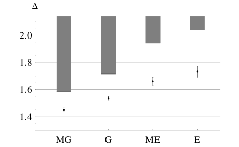
Figure 1: Values of $\Delta$ for media in Table 1 (note reordering). Shaded bars: region excluded by replica bounds. Symbols: numerical results (error bars indicate combined statistical and systematic uncertainty).

VI Discussion

Motivated by the problem of Huygens-front propagation in isotropic random media, which reduces to previously studied white-noise systems (Burgers turbulence and directed polymers) in the weak-perturbation limit, we have performed a systematic study to obtain quantitative information about the front speedup via the prefactor $\Delta$ of the already established $\epsilon^{4/3}$ scaling Mayo and Kerstein (2007). The prefactor $\Delta$ corresponds to the energy density of the Burgers fluid and the binding energy of the directed polymer, making these “toy models” directly applicable to the propagation problem. The latter, though also idealized, is physically more realistic because, e.g., white noise is not assumed. We have extended the variational analysis based on the replica method—previously applied to directed polymers Mézard and Parisi (1991); Goldschmidt (1993); Blum (1994) and then to Burgers turbulence Bouchaud et al. (1995)—with a specific focus on the value of $\Delta$ in the zero-temperature or inviscid limit, corresponding to Huygens propagation. This analysis has been found sufficiently tractable to yield explicit upper bounds on $\Delta$ for arbitrary perturbation spectra $D(k)$, subject to the previously identified conditions Mayo and Kerstein (2007) for reduction of the propagation problem to white noise.

Let us summarize how the numerical value of the replica bound on $\Delta$ can be obtained for a $d$-dimensional random medium with a particular spectrum $D(k)$, either specified analytically or determined from an experiment or simulation to sufficient precision to perform the required computations. [A turbulent energy spectrum $E(k)$ can be converted to an equivalent quenched-medium spectrum using Eq. (79).] First we obtain the functions $B_{p}(z)$ from Eq. (36) for $p=0$, $1$, $2$, $3$, and define $\mu(z)$ by Eq. (45). A general replica bound formula is then Eq. (65), where $z_{*}\geq 0$ is such that $\mu(z)$ is a decreasing function for $0<z<z_{*}$. If $\mu(z)$ is decreasing for all $z>0$, we can take $z_{*}=\infty$ and use a simpler formula, Eq. (58). An alternative bound applicable in all cases, which may be better or worse (or even completely uninformative), is the “one-step” result, Eq. (75). Heuristically, the one-step bound tends to dominate for single-scale media in high dimensions or in which low wave numbers are suppressed (the two are related because the “volume” of low wave numbers has a $k^{d}$ factor).

The replica results are particularly interesting in light of rigorous properties of random Huygens propagation that have been deduced from general arguments. The dependence of the replica bounds on the form of the spectrum (confirmed by numerical results) indicates that the rigorous bound on relative speedup derived in Sec. III.1 is not usefully sharp when applied to spectra of different shapes. The replica bounds, at least for one class of media, are consistent with the fact that a lower-dimensional “slice” through a medium has a smaller (or equal) speedup due to elimination of some possible paths. For randomly advected Huygens propagation (considered as an idealization of turbulent combustion), monotonicity with respect to the laminar flame speed $u_{L}$, in conjunction with the finite replica bound for weak $\mathrm{Re}=\infty$ turbulence, precludes a divergent turbulent burning velocity $u_{T}$ in strong $\mathrm{Re}=\infty$ turbulence ($u_{L}\to 0$).

The key qualitative insight obtained from the analytic form of the replica bounds is the concept of finite-band renormalization. The picture of a progressively coarse-grained medium with an upwardly renormalized propagation speed has been previously used in turbulent combustion Yakhot (1988); Pocheau (1994), but it was assumed that the renormalization is purely local in wave number, i.e., that the effect on the renormalized speed $u_{R}$ of eliminating an arbitrarily narrow high-wave-number band depends only on the spectral power $\phi$ in that band. On dimensional grounds, then, the change in renormalized speed is

$$\delta u_{R}\propto u_{R}\left(\frac{\phi}{u_{R}^{2}}\right)^{r/2},$$ (86)

where we assume that the dependence on $\phi$ is a power law. If the spectrum consisted only of the band in question, then Eq. (86) would have to reproduce the weak-perturbation speedup scaling (now known to be $r=\frac{4}{3}$). Equation (86) can be rewritten as a simple additive renormalization,

$$\delta(u_{R}^{r})\propto\phi^{r/2}.$$ (87)

It was then argued Pocheau (1994) that in turbulent combustion, the effect of eliminating many such bands in succession, covering an entire spectrum, would be to increase $u_{R}$ from $u_{L}$ to $u_{T}$, with a cumulative renormalization of $u_{R}^{r}$ proportional to $(u^{\prime 2})^{r/2}$ (where $u^{\prime 2}$ is the total spectral power), giving

$$u_{T}^{r}-u_{L}^{r}\propto u^{\prime r}.$$ (88)

This formula has the encouraging feature that $u_{T}\propto u^{\prime}$ for $u_{L}\to 0$, as expected.

We observe, however, that the use of arbitrarily narrow wave-number bands is incompatible with $r=\frac{4}{3}$. If the spectrum is divided into $M$ bands of equal power $\phi=u^{\prime 2}/M$, then the effect of $M$ renormalizations by Eq. (87) is

$$u_{T}^{r}-u_{L}^{r}\propto M\left(\frac{u^{\prime 2}}{M}\right)^{r/2},$$ (89)

which has a finite limit as $M\to\infty$ only if $r=2$. This exponent value, corresponding to an $\epsilon^{2}$ weak-perturbation speedup, was in fact suggested by an earlier field-theoretic renormalization analysis based on infinitesimal wave-number bands Yakhot (1988), which is widely used as a model of $u_{T}$. That analysis, besides having the wrong weak-turbulence scaling, predicts that $u_{T}$ depends only on $u_{L}$ and $u^{\prime}$ but not on the form of the spectrum, in contradiction to the nonuniversality (spectrum dependence) seen in our analytical and numerical results.

The unsuitability of infinitesimal bands for analyzing Huygens propagation is seen not only formally but also physically. The rationale for stepwise renormalization is that the front reaches a steady state with respect to small-scale perturbations, thereby determining the effective speed of a coarse-grained front that responds to larger-scale perturbations. This picture is literally applicable if the perturbations exist on two widely separated scales. For continuous spectra, such renormalization is approximately justified if the bands are wide enough to give significant scale separation, but narrow enough to be roughly monochromatic so that spectral shape is not an issue within each band. Thus it is not surprising that the replica bounds involve the power in an order-unity band, Eq. (60).

Front-speed renormalization has here been placed on a sounder footing by means of the replica method, but only in the weak-perturbation limit. It is tempting to conjecture that a relation like Eq. (88) with $r=\frac{4}{3}$ may still hold beyond that limit, with $u_{T}^{4/3}-u_{L}^{4/3}$ given by a quantity characterizing the random advection. This would imply that the weak-turbulence speedup prefactor $\Delta$ can be used to determine the strong-turbulence value of $u_{T}$ by taking $u_{L}\to 0$. Such a relation, however, is incompatible with the expectation that $u_{T}$ in strong turbulence depends not only on the spectrum (or two-point spatial correlation function), which completely determines $\Delta$, but also on other flow properties including time dependence and higher moments. Time dependence clearly can affect $u_{T}$ because, e.g., if the flow correlation time goes to zero at fixed $u^{\prime}$ and $u_{L}$, then the turbulent diffusivity vanishes and the effect of advection disappears. Dependence on only the two-point spatial correlation function is an asymptotic result of the central limit theorem for $u^{\prime}/u_{L}\to 0$ and does not apply beyond that regime Mayo and Kerstein (2007). Thus a relation like Eq. (88) can hold only for a restricted class of flows, if at all. More generally, it is not yet clear whether the finite-band renormalization concept is useful beyond the weak-perturbation limit.

Because the accuracy of the replica bounds on $\Delta$ is not rigorously established in general, it is important to seek independent validation. To this end, we have presented the results of high-precision numerical simulations of the one-dimensional inviscid KPZ-Burgers equation with white-in-time forcing, which corresponds to two-dimensional Huygens propagation. The numerical results are within about 15% of the replica bounds for four example media. Although the replica method has been validated rigorously for spin glasses Guerra (2003); Talagrand (2006), the present work is the only quantitative test of directed-polymer replica bounds known to us.

High-precision simulations in a greater number of dimensions would be very costly. Well-controlled experiments would be an alternative way to validate the replica results for three-dimensional propagation. One speculative possibility is based on reinterpreting the function $T_{0}$ appearing in the eikonal equation (90) as an electrostatic potential. If a heterogeneous ferroelectric medium can be constructed in which the electric field $-\bm{\nabla}T_{0}$ at each point has a frozen magnitude $\propto 1+\sigma(\mathbf{x})$ but an unconstrained direction, then one face of the medium can be grounded ($T_{0}=0$), which determines the electric-field direction throughout the medium, and the potential can be measured along the opposite face to determine the “speedup.” (A small dissipative term $\propto\nabla^{2}T_{0}$ is needed in the eikonal equation to regulate singularities in accordance with Huygens’ principle, and so the local charge density must affect the mechanism that freezes the local electric-field magnitude.) By whatever technique, confirmation of the sharpness of the replica bounds for three-dimensional propagation under idealized conditions would establish these bounds as an appropriate starting point and limiting case for more complex and realistic engineering models, such as are needed in turbulent combustion. Other physical applications were noted previously Mayo and Kerstein (2007).

Appendix A Applicability of the KPZ equation

In Sec. II we assumed that the KPZ equation (2) adequately describes the propagation of an initially flat front in a quenched medium with weak random fluctuations. Here, the justification of this assumption is explained. An exact equation for Huygens propagation in a quenched medium is the eikonal equation Mayo and Kerstein (2007)

$$|\bm{\nabla}T_{0}|=1+\sigma,$$ (90)

where $T_{0}(\mathbf{x})$ is the arrival time at a point $\mathbf{x}$ and $\sigma(\mathbf{x})$ is the refractive-index fluctuation. If we define $h(x_{\parallel},\mathbf{x}_{\perp})=x_{\parallel}-T_{0}(x_{\parallel},\mathbf{x}_{\perp})$ in accordance with Eq. (6) and assume that the overall propagation is in the $+x_{\parallel}$-direction, then the eikonal equation can be written

$$\frac{\partial h}{\partial x_{\parallel}}=1-\sqrt{(1+\sigma)^{2}-|\bm{\nabla}_{\perp}h|^{2}}.$$ (91)

In an initial interval of $x_{\parallel}$ where $|\bm{\nabla}_{\perp}h|^{2}$ is small compared to typical values of $\sigma$, the right-hand side of Eq. (91) equals $-\sigma$ to leading order. Thus the tilt $\bm{\nabla}_{\perp}h$, initially zero, grows with $x_{\parallel}$ at a rate proportional to the amplitude of $\sigma$ (measured by the rms fluctuation $\epsilon\ll 1$), executing a random walk as new, uncorrelated fluctuations are encountered. It follows that $|\bm{\nabla}_{\perp}h|^{2}$ remains smaller than $\epsilon$ for at least a distance of order $\epsilon^{-1}$. (This is a conservative estimate because cusp formation, equivalent to discarding certain branches of a multivalued eikonal solution, can and does eliminate relatively large tilts.)

But the rescaling of $x_{\parallel}$ performed in Sec. II.2 shows that the characteristic distance for front equilibration is of order $\epsilon^{-2/3}\ll\epsilon^{-1}$. Thus, at a minimum, our approximation $|\bm{\nabla}_{\perp}h|^{2}\ll\epsilon$ remains valid well after a statistically steady state is reached, and its validity is then assured forever. Nonetheless, the contribution of $|\bm{\nabla}_{\perp}h|^{2}$ must be included in a useful reduced equation for propagation, because this nonlinear term is responsible for producing the steady state. The leading terms in Eq. (91) then give the inviscid KPZ equation

$$\frac{\partial h}{\partial x_{\parallel}}=\tfrac{1}{2}|\bm{\nabla}_{\perp}h|^{2}-\sigma;$$ (92)

the omitted terms are negligible compared to $|\bm{\nabla}_{\perp}h|^{2}$. We conclude that the formation and properties of the Huygens-propagation steady state (for sufficiently small $\epsilon$) are accurately described by the KPZ equation with a non-white-noise perturbation $-\sigma$ and with viscosity taken to zero.

Appendix B Gaussian trial functions and replica symmetry breaking

To allow the expectation value $\langle\psi|\mathcal{H}_{n}|\psi\rangle$ of the $n$-particle Hamiltonian (23) to be expressed analytically in $n$, we adopt the usual isotropic Gaussian trial wave functions

$$\psi(\mathbf{y}_{1},\dotsc,\mathbf{y}_{n})\propto\exp\biggl{(}-\tfrac{1}{4}\sum_{a,b=1}^{n}(Q^{-1})_{ab}\,\mathbf{y}_{a}\cdot\mathbf{y}_{b}\biggr{)},$$ (93)

which obey $\langle\psi|\,\mathbf{y}_{a}\cdot\mathbf{y}_{b}\,|\psi\rangle=(d-1)Q_{ab}$, where $Q$ is a positive-definite matrix. For positive integer $n$, the optimal choice of $Q$ to approximate the ground state would be invariant under arbitrary permutations of the replicas, because this is a symmetry of the Hamiltonian. For $n\to 0$, however, at least within this variational approach, the permutation invariance is violated through hierarchical replica symmetry breaking Mézard et al. (1987); Mézard and Parisi (1991). The hierarchical matrix $Q$ is constructed as follows, starting from positive integer $n$. Given integers $1\equiv m_{0}\leq m_{1}\leq\dotsb\leq m_{K}\leq m_{K+1}\equiv n$ such that each $m_{i}$ divides $m_{i+1}$, define $M_{i}$ as the $n\times n$ block-diagonal matrix consisting of submatrices of size $m_{i}\times m_{i}$ with all entries $1$ (e.g., $M_{0}$ is the identity matrix). Then define

$$Q=\sum_{i=0}^{K+1}b_{i}M_{i},$$ (94)

where the scalars $b_{i}$ have dimensions $\mathsf{L}^{2}$. The $n$ particles are thus divided into blocks, sub-blocks, etc., that are bound on different length scales; this already suggests a connection to renormalization ideas.

Because all the $M_{i}$ are seen to commute, the eigenvalues of $Q$ are readily found. Each all-$1$ submatrix of $M_{i}$ has one eigenvalue $m_{i}$ and $m_{i}-1$ eigenvalues $0$, so $M_{i}$ has $n/m_{i}$ eigenvalues $m_{i}$ and $n-n/m_{i}$ eigenvalues $0$. For $0\leq i\leq K$, the matrix $Q$ has $n/m_{i}-n/m_{i+1}$ eigenvectors that are in the null space of $M_{j}$ for $j>i$ but in the nonzero eigenspace of $M_{j}$ for $j\leq i$. Thus an eigenvalue of $Q$ with multiplicity $n/m_{i}-n/m_{i+1}$ is

$$\Lambda_{i}=\sum_{j=0}^{i}b_{j}m_{j}.$$ (95)

It is convenient to define piecewise constant functions on the real interval $1<u\leq n$:

$$\Lambda(u) =\Lambda_{i} (m_{i}<u\leq m_{i+1}),$$ (96)

$$z(u) =2\sum_{j=0}^{i}b_{j} (m_{i}<u\leq m_{i+1}),$$ (97)

so that

$$\Lambda(u)=\tfrac{1}{2}u\,z(u)-\tfrac{1}{2}\int_{1}^{u}dv\,z(v).$$ (98)

There is a single further eigenvalue of $Q$ given by Eq. (95) with $i=K+1$, corresponding to the eigenvector $(1,\dotsc,1)$. This represents a center-of-mass translation, and the eigenvalue $\Lambda_{K+1}$ should go to infinity in the ground state (complete freedom of the center of mass).

We can interpret $z(m_{i})=2\sum_{j=0}^{i-1}b_{j}$ as the variance of each component of interparticle separation,

$$z(m_{i})=\langle\psi|\,[\hat{\mathbf{n}}\cdot(\mathbf{y}_{a}-\mathbf{y}_{b})]^{2}\,|\psi\rangle=Q_{aa}+Q_{bb}-2Q_{ab},$$ (99)

for indices $a$ and $b$ that are in the same size-$m_{i}$ block but different size-$m_{i-1}$ blocks. [We see this because, from Eq. (94), $Q_{aa}=Q_{bb}=\sum_{j=0}^{K+1}b_{j}$ and $Q_{ab}=\sum_{j=i}^{K+1}b_{j}$.] Using the Gaussian identity (17), this time with $\zeta=i\mathbf{k}_{\perp}\cdot(\mathbf{y}_{a}-\mathbf{y}_{b})$, it follows that

$$\langle\psi|\exp[i\mathbf{k}_{\perp}\cdot(\mathbf{y}_{a}-\mathbf{y}_{b})]\,|\psi\rangle=\exp[-\tfrac{1}{2}|\mathbf{k}_{\perp}|^{2}\,z(m_{i})].$$ (100)

Then, from Eq. (20), we obtain

$$\begin{split}&\langle\psi|\,V(|\mathbf{y}_{a}-\mathbf{y}_{b}|)\,|\psi\rangle\\ &\qquad=\int\frac{d^{d-1}\mathbf{k}_{\perp}}{(2\pi)^{d-1}}\,\exp[-\tfrac{1}{2}|\mathbf{k}_{\perp}|^{2}\,z(m_{i})]\,D(|\mathbf{k}_{\perp}|)\\ &\qquad\equiv B_{0}\bm{(}z(m_{i})\bm{)},\end{split}$$ (101)

where the function $B_{0}$ is determined by the spectrum of the random medium. The number of index pairs $(a,b)$ of the type considered is $n(m_{i}-m_{i-1})$; the range $1\leq i\leq K+1$ covers all pairs with $a\neq b$. There are an additional $n$ self-pairs ($a=b$) for which, in place of Eq. (101), we have $\langle\psi|\,V(0)\,|\psi\rangle=B_{0}(0)$. Thus

$$\begin{split}&\sum_{a,b=1}^{n}\langle\psi|\,V(|\mathbf{y}_{a}-\mathbf{y}_{b}|)\,|\psi\rangle\\ &\qquad=n\,B_{0}(0)+\sum_{i=1}^{K+1}n(m_{i}-m_{i-1})\,B_{0}\bm{(}z(m_{i})\bm{)}\\ &\qquad=n\left(B_{0}(0)+\int_{1}^{n}du\,B_{0}\bm{(}z(u)\bm{)}\right).\end{split}$$ (102)

Meanwhile, for the kinetic part of the Hamiltonian, we find

$$\begin{split}\sum_{a=1}^{n}\langle\psi|\nabla_{a}^{2}|\psi\rangle&=-\tfrac{1}{4}(d-1)\operatorname{tr}Q^{-1}\\ &=-\tfrac{1}{4}(d-1)\sum_{i=0}^{K}\left(\frac{n}{m_{i}}-\frac{n}{m_{i+1}}\right)\frac{1}{\Lambda_{i}}\\ &=-\tfrac{1}{4}(d-1)n\int_{1}^{n}\frac{du}{u^{2}\,\Lambda(u)},\end{split}$$ (103)

where we have set $1/\Lambda_{K+1}=0$. Combining these results, we obtain the expectation value of the Hamiltonian (23),

$$\begin{split}\langle\psi|\mathcal{H}_{n}|\psi\rangle={}&\tfrac{1}{8}\tau^{2}(d-1)n\int_{1}^{n}\frac{du}{u^{2}\,\Lambda(u)}\\ &-\frac{n}{2\tau}\left(B_{0}(0)+\int_{1}^{n}du\,B_{0}\bm{(}z(u)\bm{)}\right).\end{split}$$ (104)

This expression is very similar to the one obtained in a replica treatment of directed polymers focused on the Gaussian medium Blum (1994). There, however, the factor $\frac{1}{2}$ multiplying the $B_{0}$ terms was incorrectly omitted. Also, the self-interaction term $\propto B_{0}(0)$ was not shown (a constant offset that does not affect the variational optimization but is important for absolute energy values); the factor $1/\tau$ in Eq. (24) was included in the definition of the Hamiltonian $\mathcal{H}_{n}$; and the following notations were used: $N=d-1$, $\beta=1/\tau$, $\lambda(u)=[2\,\Lambda(u)]^{-1}$, $Q(u)=z(u)$, $\hat{f}=-B_{0}/(d-1)$.

In the formal limit $n\to 0$, the block “sizes” $m_{i}$ are assumed to be real numbers in the reversed sequence $n\equiv m_{K+1}\leq m_{K}\leq\dotsb\leq m_{1}\leq m_{0}\equiv 1$, with arbitrarily large $K$ and no divisibility constraints. As $K\to\infty$, then, $\Lambda(u)$ and $z(u)$ become general functions on the interval $0<u<1$. Because $\Lambda(u)$ represents an eigenvalue of $Q$ and $z(u)$ represents a variance, both must be nonnegative. A further constraint arises when we require nonnegativity of variances involving arbitrary numbers of particles from various blocks (arbitrary because, upon analytic continuation in $n$, there is no limit on the number of particle indices that can be formally considered, unlike the case of positive integer $n$). The parameters $b_{i}$, which determine the matrix elements of $Q$, must be such that all eigenvalues $\Lambda(u)$ are nonnegative, not just for $n\to 0$ but also for arbitrary realizable integer values $1\equiv m_{0}\leq\dotsb\leq m_{K+1}\equiv n$. From Eq. (95), we see that nonnegativity of $\Lambda_{i}$ for arbitrarily large $m_{i}$ requires $b_{i}\geq 0$. Consequently $z(u)$, as defined in Eq. (97), is a nondecreasing function for $1<u<n$; and so in the $n\to 0$ limit, where the order of the $m_{i}$ is reversed, $z(u)$ must be a nonincreasing function for $0<u<1$. In fact, from Eq. (98) and its implication

$$\Lambda^{\prime}(u)=\tfrac{1}{2}u\,z^{\prime}(u),$$ (105)

a nonnegative and nonincreasing function $z(u)$ will produce a function $\Lambda(u)$ with the same properties.

Appendix C Numerical method for the inviscid KPZ equation

We simulate the one-dimensional inviscid KPZ equation (85) by a Lagrangian finite-element method in which the only approximation, aside from the periodic domain, is a time and space discretization of the white noise $\eta$. Equation (85) itself is solved exactly (except for roundoff error). We solve this equation, rather than just the Burgers equation obtained from it, because $h$ remains continuous at shocks and can be used to track them, and because computing $h$ allows use of the formula $\Delta=\langle\partial h/\partial t\rangle$ (in which averaging over $t$ is particularly convenient). The time discretization of $\eta$ is in a sense the simplest possible: a sequence of “delta-function kicks” at equally spaced instants $t_{k}=kb$ with $k=1$, $2$, $\dotsc$. Each kick has a random $x$ profile (of a form to be described) and an overall amplitude that scales with $b^{1/2}$, to produce white noise as $b\to 0$.

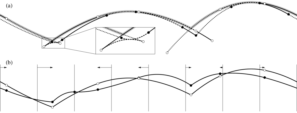
Figure 2: Lagrangian finite-element method for the inviscid KPZ equation. Plots show stages in the simulated evolution of $h(x)$ on a periodic $x$ domain. (a) Filled circles bound quadratic elements of the initial configuration, distinguished by alternating dotted, dashed, and solid curves. One initial cusp is present, in the right half of the plot. After advection of all boundaries, $h(x)$ consists of corresponding elements bounded by open circles, and is no longer single-valued. The filled circle at the initial cusp separates into two open circles, and a dashed element in the left half of the plot turns inside out when its boundaries pass through one another (inset). The trimming procedure then constructs a single-valued $h(x)$ by retaining only the largest values (shaded band). As a result, a solid element disappears into the existing cusp, and the inside-out dashed element disappears to form a new cusp. (b) Open circles indicate trimmed element boundaries from (a), including updated cusp locations. Vertical lines form grid for kicking. Arrows indicate deformation of kicking boundaries to existing element boundaries, except third grid line from left, which has no nearby element boundary and introduces a new one. Kicking produces elements bounded by filled circles, without altering the number or location of cusps. This final $h(x)$ can then be evolved again as in (a).

The steps in our numerical method are displayed in Fig. 2. We represent a “snapshot” of $h(x)$ by a piecewise quadratic function on various $x$ intervals (elements). Continuity of $h$ is required, but $\partial h/\partial x$ can jump discontinuously upward at shocks (corresponding to Huygens cusps that are concave, not convex). Between kicks, the elements evolve dynamically in a way that preserves the piecewise quadratic form. Specifically, the nonlinear term $\frac{1}{2}(\partial h/\partial x)^{2}$ in Eq. (85) is quadratic in $x$ if $h$ is, and so when $\eta=0$ the exact solution remains in the piecewise quadratic space. Element boundaries without shocks are simply advected at the local Burgers velocity $w=-\partial h/\partial x$ (which is constant along Lagrangian trajectories) Sethian (1985). For boundaries with shocks, the adjacent segments are at first allowed to overlap. Even with no shocks initially, elements can overlap if boundaries pass through one another, indicating formation of a new shock.

In this way $h(x)$ can be evolved directly to the time of the next kick, but it generally becomes multivalued, consisting of quadratic functions on overlapping $x$ intervals. The solution is then “trimmed” to obtain nonoverlapping elements containing the largest value of $h$ at each $x$, as illustrated in Fig. 2(a). Some elements are cut down; others are discarded entirely (such as those that turn inside out when a new shock forms). The portions removed can be interpreted as Burgers fluid elements that have run into shocks or as segments of the Huygens front that have been overtaken at cusps. The trimming procedure is tractable if no overlaps occur between elements that were more distant than next-to-nearest neighbors. If this condition is violated, we split the time interval in half and perform the evolution in two stages, recursively. Because the configuration of $h(x)$ results from a random process, the next-to-nearest interaction is in fact sufficient for evolution over a finite time interval. That is, barring exact synchronization between different parts of space (which is vanishingly unlikely), any overlap of more distant elements can be reduced to discrete stages of evolution in which only nearest and next-to-nearest neighbors overlap. For example, a shock gradually absorbs the elements on either side of it (say elements $1$ and $2$), but one of the two will disappear first, resulting in a renumbering of the remaining elements. Only if they disappeared at the same instant would we have an unavoidable interaction between elements $0$ and $3$.

“Kicking,” illustrated in Fig. 2(b), preserves the assumed form of $h(x)$ if the spatial profile of the kick is also piecewise quadratic. Such a profile is synthesized from a given spectrum $D(k)$ by first generating delta-function spikes on a uniform $x$ grid (spacing $\delta$) based on a spectrum $k^{6}\,D(k)$, and then forming a smooth piecewise quadratic function by in effect analytically integrating three times with respect to $x$. (This kick profile has an everywhere continuous derivative to avoid introducing additional shocks, especially ones of unphysical sign.) The choice of the forcing grid is the only way in which a finite spatial resolution $\delta$ enters the simulation. As described, the kicking process would introduce a new element boundary in $h(x)$ at every grid point, since generically every boundary introduced in a previous kick has moved at least slightly. Each boundary survives for some characteristic timescale before vanishing into a shock, and so the steady-state average number of boundaries present is proportional to the rate at which they are introduced, which would scale with the kicking rate $1/b$. As we take $b\to 0$ to represent white noise accurately, we would have an explosion in the number of elements, but they would be mostly redundant since the spatial resolution of the driving noise is still limited by the grid. We adopt a more efficient approach that adds a new boundary only when $h(x)$ is insufficiently resolved in the neighborhood of the point in question, and otherwise deforms the kick so as to take advantage of an existing nearby boundary rather than insisting on the planned grid. The small-scale deformation distorts the high-wave-number part of the noise spectrum and thus requires a somewhat finer grid to achieve the same accuracy. But the cost is outweighed by the much-improved behavior as $b\to 0$: Now the average number of boundaries remains fixed.

Conventional numerical methods for the Burgers-KPZ and similar equations require fine spatial grids to resolve shocks, and nonzero viscosity to stabilize them. By contrast, we take the inviscid limit from the start, allowing an explicit geometric representation of shocks. The spatial grid need only resolve the forcing; inviscid shocks are perfectly sharp and do not introduce smaller length scales. If the forcing is spatially smooth (as for media G and MG), then there is a significant advantage in efficiency from using a relatively coarse grid and still capturing sharp shocks. With spatially rough forcing (i.e., a spectrum with a long high-wave-number tail, as for media E and ME), the advantage is less clear because a fine grid is needed anyway to resolve the forcing accurately. Nevertheless, because we work directly at $\mathrm{Re}_{\text{B}}=\infty$, there is one fewer parameter contributing systematic errors. Our method is designed explicitly for a one-dimensional simulation ($d=2$); generalization to the Burgers-KPZ equation in two or more dimensions ($d\geq 3$) is possible in principle, but the computational geometry would be much more intricate and possibly intractable. As with conventional methods, the computational cost of simulations in higher dimensions would be severe.

We now describe how the parameters of our simulations are chosen and how the uncertainties in the results are estimated. By systematic error we mean the difference between the precise average of a quantity over many runs of a practical simulation (where each run takes a finite computation time) and the precise average for the idealized problem statement (where space and time are considered infinite and continuous). An efficient computational approach involves balancing statistical and systematic errors, both of which contribute to the overall uncertainty of the result. In our case, the relevant systematic parameters that ideally approach infinity are $L$, $1/\delta$, $1/b$, and the time $T$ allowed for equilibration before data are taken. We estimate $\Delta$ by subsequently averaging $\partial h/\partial t$ over a time interval $3T$, based on the following considerations: It cannot be efficient to spend much more time on equilibration than on averaging, and even if it were ideal to spend only a tiny fraction of the computation time on equilibration, spending $\frac{1}{4}$ on it reduces the available data for averaging only modestly, increasing the statistical error by $(\frac{4}{3})^{1/2}-1\simeq 15\%$.

Our framework for treating systematic errors is a conservative assumption that these errors scale with the reciprocal of the parameters given above. (This is the slowest convergence that we would reasonably anticipate.) That is, we assume that the precise average computed from many runs of a simulation tends to the true value of $\Delta$ with asymptotic corrections of order $1/L$, order $\delta$, order $b$, and order $1/T$. Consequently, we can extrapolate from simulations performed with different finite parameters to estimate the result of an ideal simulation. Because we do not trust this extrapolation as a quantitative model, we will apply it only when all the simulation results contributing to the extrapolation are statistically indistinguishable (consistent with identical underlying averages).

Specifically, our final extrapolation will be based on a “most refined” simulation, with parameter set $\alpha$, and $N=4$ lesser simulations $\beta_{0}$, $\dotsc$, $\beta_{N-1}$, each based on $\alpha$ with one parameter halved. All these simulations are repeated as necessary to obtain averages $A$ and $B_{i}$ with some statistical uncertainty $\sigma$ (to be determined below). Because of the parameter halving and the assumed reciprocal scaling of systematic errors, the extrapolation takes the simple form

$$\Delta\simeq A+(A-B_{0})+\dotsb+(A-B_{N-1}).$$ (106)

To ensure that the result is fairly insensitive to our specific model of systematic errors, we require each correction term $A-B_{i}$ to be within two standard deviations of zero, i.e.,

$$\lvert A-B_{i}\rvert\leq 2\sqrt{2}\,\sigma.$$ (107)

(Taking a difference of two independent random variables multiplies the standard deviation by $\sqrt{2}$.) If the decay of systematic errors is more rapid than assumed, Eq. (106) is needlessly imprecise but not incorrect, because the exaggerated correction terms are statistically equivalent to zero. Our final estimate of $\Delta$, being a sum of independent random variables $(N+1)A-B_{0}-\dotsb-B_{N-1}$, has a variance $[(N+1)^{2}+N]\sigma^{2}=29\sigma^{2}$. Thus $\sigma$ should be taken as the desired overall uncertainty divided by $\sqrt{29}$. By repeated doubling, we can locate a parameter set $\alpha$ sufficiently refined that Eq. (107) holds.

The purpose of the extrapolation method is to obtain a conservative assessment of the uncertainty contributed by systematic errors. Our procedure is qualitatively similar to traditional rules of thumb, such as, “The change in the simulation result upon doubling the resolution is an estimate of the systematic uncertainty.” But the somewhat arbitrary technique of doubling the resolution (or other parameters) is replaced here by a more fundamental assumption about the scaling of systematic errors. (In simpler problems, such as the finite-difference solution of deterministic differential equations, the correct scaling can be readily obtained by analysis, but we desire a robust “black box” method.)

Table 3: Most refined numerical simulation parameters, and resulting extrapolated estimate of $\Delta$, for media in Table 1 (with $a=1$).

Medium	$\log_{2}L$	$\log_{2}(3\delta)$	$\log_{2}b$	$\log_{2}T$	$\Delta$
G	$8$	$-2$	$-4$	$8$	$1.535(14)$
MG	$7$	$-3$	$-6$	$6$	$1.450(13)$
E	$7$	$-5$	$-5$	$5$	$1.73(4)$
ME	$6$	$-5$	$-5$	$4$	$1.66(3)$

For each of our four example spectra, Table 3 gives the parameters $\alpha$ of the most refined simulation performed, and the resulting extrapolated estimate of $\Delta$ including both statistical and systematic uncertainties.

References

- Kerstein and Ashurst (1994) A. R. Kerstein and W. T. Ashurst, Phys. Rev. E 50, 1100 (1994).
- Mayo and Kerstein (2007) J. R. Mayo and A. R. Kerstein, Phys. Lett. A 372, 5 (2007).
- Gomes et al. (2005) D. Gomes, R. Iturriaga, K. Khanin, and P. Padilla, Moscow Math. J. 5, 613 (2005).
- Bouchaud et al. (1995) J. P. Bouchaud, M. Mézard, and G. Parisi, Phys. Rev. E 52, 3656 (1995).
- Mézard and Parisi (1991) M. Mézard and G. Parisi, J. Phys. I (France) 1, 809 (1991).
- Goldschmidt (1993) Y. Y. Goldschmidt, Nucl. Phys. B 393, 507 (1993).
- Blum (1994) T. Blum, J. Phys. A 27, 645 (1994).
- Kardar et al. (1986) M. Kardar, G. Parisi, and Y.-C. Zhang, Phys. Rev. Lett. 56, 889 (1986).
- Feynman and Hibbs (1965) R. P. Feynman and A. R. Hibbs, Quantum Mechanics and Path Integrals (McGraw-Hill, New York, 1965).
- Williams (1985) F. A. Williams, Combustion Theory (Benjamin/Cummings, Menlo Park, California, 1985), 2nd ed.
- Crandall and Lions (1983) M. G. Crandall and P.-L. Lions, Trans. Am. Math. Soc. 277, 1 (1983).
- Sethian (1985) J. A. Sethian, Commun. Math. Phys. 101, 487 (1985).
- Roth et al. (1993) M. Roth, G. Müller, and R. Snieder, Geophys. J. Int. 115, 552 (1993).
- Kerstein and Ashurst (1992) A. R. Kerstein and W. T. Ashurst, Phys. Rev. Lett. 68, 934 (1992).
- Iturriaga and Khanin (2003) R. Iturriaga and K. Khanin, Commun. Math. Phys. 232, 377 (2003).
- Edwards and Anderson (1975) S. F. Edwards and P. W. Anderson, J. Phys. F 5, 965 (1975).
- Binder and Young (1986) K. Binder and A. P. Young, Rev. Mod. Phys. 58, 801 (1986).
- den Hollander and Toninelli (2005) F. den Hollander and F. Toninelli, Eur. Math. Soc. Newsl. 56, 13 (2005).
- Mézard and Parisi (1992) M. Mézard and G. Parisi, J. Phys. A 25, 4521 (1992).
- Guerra (2003) F. Guerra, Commun. Math. Phys. 233, 1 (2003).
- Talagrand (2006) M. Talagrand, Ann. Math. 163, 221 (2006).
- Sendiña-Nadal et al. (1998) I. Sendiña-Nadal, A. P. Muñuzuri, D. Vives, V. Pérez-Muñuzuri, J. Casademunt, L. Ramírez-Piscina, J. M. Sancho, and F. Sagués, Phys. Rev. Lett. 80, 5437 (1998).
- Gotoh and Kraichnan (1998) T. Gotoh and R. H. Kraichnan, Phys. Fluids 10, 2859 (1998).
- Gotoh (1999) T. Gotoh, Phys. Fluids 11, 2143 (1999).
- (25) T. Gotoh, private communication.
- Yakhot (1988) V. Yakhot, Combust. Sci. Tech. 60, 191 (1988).
- Pocheau (1994) A. Pocheau, Phys. Rev. E 49, 1109 (1994).
- Mézard et al. (1987) M. Mézard, G. Parisi, and M. A. Virasoro, Spin Glass Theory and Beyond (World Scientific, Singapore, 1987).