An Economic Model of Coupled Exponential Maps

Abstract

In this work, an ensemble of economic interacting agents is considered. The agents are arranged in a linear array where only local couplings are allowed. The deterministic dynamics of each agent is given by a map. This map is expressed by two factors. The first one is a linear term that models the expansion of the agent’s economy and that is controlled by the growth capacity parameter. The second one is an inhibition exponential term that is regulated by the local environmental pressure. Depending on the parameter setting, the system can display Pareto or Boltzmann-Gibbs behavior in the asymptotic dynamical regime. The regions of parameter space where the system exhibits one of these two statistical behaviors are delimited. Other properties of the system, such as the mean wealth, the standard deviation and the Gini coefficient, are also calculated.

I Introduction

Nowadays it is well established that the wealth distribution in western societies presents essentially two phases. This means that the whole society can be split in two disjoint parts in which the richness distribution is different in each of them. Thus, Dragulescu and Yakovenko [1] have found, over real economic data from UK and USA societies, that one phase presents an exponential (Boltzmann-Gibbs $\rightarrow$ BG) distribution which covers about $95\%$ of individuals, those with low and medium incomes, and that the other phase, which is integrated by the high incomes, i.e., the $5\%$ of individuals, shows a power (Pareto) law. Different dynamical mechanisms for the interaction among agents in multi-agent economic models have been proposed in the literature in order to reproduce these two types of statistical behavior.

In the Dragulescu and Yakovenko [2] model, a set of $N$ economic agents exchange their own amount of money $u_{i}$, with $i=1,2,\cdots,N$, under random binary $(i,j)$ interactions, $(u_{i},u_{j})\rightarrow(u_{i}^{\prime},u_{j}^{\prime})$, by the following exchange rule:

$$u^{\prime}_{i} = \epsilon(u_{i}+u_{j}),$$ (1)

$$u^{\prime}_{j} = \bar{\epsilon}(u_{i}+u_{j}),$$ (2)

with $\bar{\epsilon}=(1-\epsilon)$, and $\epsilon$ a random number in the interval $(0,1)$. Starting the system from an initial state with equity among all the agents, it evolves towards an asymptotic dynamical state where the richness follows a BG distribution [3]. This model is equivalent to the saving propensity model introduced by Chakraborti and Chakrabarti [4] for the particular case in which the agents do not save any fraction of money before carrying out each transaction. A similar model was introduced by Angle [5]. In this case, the random pair $(i,j)$ of economic agents, $(u_{i},u_{j})$, exchanges money under the rule:

$$u^{\prime}_{i} = u_{i}-\Delta u,$$ (3)

$$u^{\prime}_{j} = u_{j}+\Delta u,$$ (4)

where

$$\Delta u=\epsilon\omega u_{i},$$ (5)

with $\epsilon$ a random number in the interval $(0,1)$. The exchange parameter, $\omega$, with $0<\omega<1$, represents the maximum fraction of wealth lost by the agent $u_{i}$ in the transaction. When $\omega=0.75$, the exponential distribution of the wealth is also found for this model.

In order to recover a power law behavior, these models can be reformulated in a nonhomogeneous way. These are models in which each agent $i$ can have assigned by some random function a different value $\omega_{i}$ of the exchange parameter $\omega$ in the Angle model [5] or a different saving propensity in the Chakraborti and Chakrabarti model [4]. Under quite general conditions, robust Pareto distributions have been found at large $u$-values in these reformulations [4, 5].

Randomness is an essential ingredient in all the former models. Thus, agents interact by pairs chosen at random, and these pairs exchange a random quantity of money in each transaction. Moreover, the transition from the BG to the Pareto behavior requires the change of the structural properties of the system. It can be reached, for instance, by introducing a strong inhomogeneity that breaks the initial indistinguishability among the units of the ensemble. From a practical point of view, this could seem an unrealistic approach since we need to conform very different setups in order to mimic the two statistical behaviors. On the other hand, interactions among the economic or social agents of a real collectivity are not fully random. In fact, they are driving in the majority of transactions by some kind of mutual interest or rational forces. Hence, it would be useful to dispose of a multi-agent model with the ability of displaying BG and Pareto behaviors emerging from an asymptotic dynamics where determinism would play some role in the evolution of the system. Now, we proceed to show with some detail the properties of one of these models[6] recently introduced in the literature.

II The Model

The model [6] consists of a linear array of $N$ interacting agents with periodic boundary conditions. Each agent, which can represent a company, country or other economic entity, is identified by an index $i$, with $i=1\cdots N$ and $N$ being the system size. Its actual state is characterized by a real number, $x_{i}$, denoting the strength, wealth or richness of the agent, with $x_{i}\in[0,\infty)$. The system evolves in time synchronously, and only interactions among nearest-neighbors are allowed. Thus, the state of the agent, $x_{i}^{t+1}$, at time $t+1$ is given by the product of two terms at the precedent time $t$; the natural growth of the agent, $r_{i}x_{i}^{t}$, with its own growth capacity parameter, $r_{i}$, and a control term that limits this growth with respect to the local field $\Psi_{i}^{t}=\frac{1}{2}(x_{i-1}^{t}+x_{i+1}^{t})$ through a negative exponential function with local environmental pressure $a_{i}$:

$$x_{i}^{t+1}=r_{i}\>x_{i}^{t}\>\exp(-\mid x_{i}^{t}-a_{i}\Psi_{i}^{t}\mid).$$ (6)

The parameter $r_{i}$ represents the capacity of the agent to become richer and the parameter $a_{i}$ describes some kind of local pressure [7] that saturates its exponential growth. This means that the largest possibility of growth for the agent is obtained when $x_{i}\simeq a_{i}\Psi_{i}^{t}$, i.e., when the agent has reached some kind of adaptation to the local environment. In this note, for the sake of simplicity, we concentrate our interest in a homogeneous system with a constant capacity $r$ and a constant selection pressure $a$ for the whole array of sites.

If all the agents start with the same wealth, the index $i$ can be omitted, $x_{i}^{t}=x^{t}$ and $\Psi_{i}^{t}=x^{t}$, and the global evolution reduces to the following map,

$$x^{t+1}=rx^{t}\exp(-\mid 1-a\mid x^{t}).$$ (7)

The above map can be easily analyzed by standard techniques. In fact, the parameter $a$ could be removed by doing the change of variable $y^{t}=\mid 1-a\mid x_{t}$, and obtaining the generic map $y^{t+1}=ry^{t}\exp(-y^{t})$. For $r<1$ the system relaxes to zero and for $r>1$ the dynamics can be self-sustained deriving toward different types of attractors. It displays all kind of bifurcations known for this type of maps [8], except, evidently, for the singular case $a=1$. For instance, when $r>1$ the fixed point is $x_{0}=\log r/\mid 1-a\mid$. This point becomes unstable by a flip bifurcation for $r=e^{2}$. For increasing $r$ the whole period doubling cascade and other complex dynamical behavior are obtained. However, it can be shown that such evolving uniform states are unstable. When a perturbation is introduced in the initial uniform state or, in general, when the initial condition is a completely random one, the asymptotic dynamical state of the system is found to be more complex.

III Some Results

We perform the statistical study of the system in the parameter space $(a,r)$. For all the simulations, the system size is $N=10^{5}$ and the initial conditions in the array are random values in the interval $(1,100)$. Also, a transient of $10^{4}$ iterations is completed before arriving to the asymptotic state where all the measurements are done. At this point, if necessary, the average is done over the next $100$ iterations after the transient, and this result is newly averaged with the same process over $100$ different realizations of the system. Following this method, different statistical quantities, such as the mean wealth, the standard deviation and the Gini coefficient, have been calculated on the model, and they will be shown in the communication to be presented in NOMA’07.

As an example, we advance here the possibility of existence of the two statistical behaviors in which we are interested in. Hence, if the number of agents, $P(x)$, with a wealth $x$ is represented in a semi-log plot, a BG distribution is found for the values $a=0.6$ and $r=4$ (Fig. 1a, where values of maps have been taken at time $t=10^{4}$). The exponent $\mu$ of this distribution, $P(x)\sim e^{-\mu x}$, is $\mu=0.26$. A thermodynamical simile can be done for this type of behavior by defining a kind of ‘temperature’, $h=1/\mu$, that is related with the mean wealth of each agent in the ensemble. In this particular case, $h=3.84$.

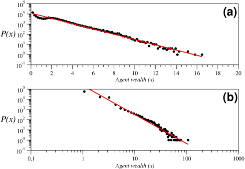
Figure 1: (1a): Semi-log plot of the number of agents, $P(x)$, with a wealth $x$ for $a=0.6$ and $r=4$ in the asymptotic regime at time $t=10^{4}$. The scaling of this exponential behavior is $0.26$. (1b): Log-log plot of $P(x)$ for $a=0.92$ and $r=8$ at time $t=10^{4}$. The exponent of this power law behavior is $2.84$.

Also, a power law behavior in the statistical behavior of system (6) is possible, for instance, for $a=0.92$ and $r=8$. If the number of agents, $P(x)$, with a wealth $x$ is now represented in a log-log plot, a Pareto distribution is unmasked [6] (Fig. 1b, where values of maps have also been taken at time $t=10^{4}$). The exponent $\alpha$ of this distribution, $P(x)\sim x^{-\alpha}$, is in this case $\alpha=2.84$, which is in clear agreement with the exponents derived from real economic data [1, 9, 10]. Thus, the exponent $\bar{\alpha}$ found in the cumulative probability distribution of incomes, whose scaling behaves as $x^{-\bar{\alpha}}\sim x^{-\alpha+1}$, is about $2.1$ for the UK and $1.7$ for the US economies [1]. Pareto himself proposed a value of $1.5$, Levy and Solomon [9] found a value of $1.36$ for the distribution of wealth in the Forbes $400$ and Souma [10] found $2.05$ for the high income distribution in Japan.

IV Conclusion

Let us conclude this note by remarking that our present model (6) shows, at least, two interesting statistical behaviors, those of Boltzmann-Gibbs and Pareto types, in its asymptotic state. The procedure to get these two regimes does not require of any structural change in the system. Only, it is necessary to tune some adequate pair of values of the external parameters $(a,r)$ for which the system displays one of those types of behavior. This property could be an advantage respect to other models in the literature that need to perform a strong change in the conformation of the initial ensemble in order to present one of the two behaviors, exponential or power law. Other relevant property of model (6) is its complete determinism. There is no any kind of random ingredient in its evolution. Of course, this does not forbid in any way that the asymptotic state of the system can show some degree of spatio-temporal complexity, including very large fluctuations of the agent’s wealth. As indicated by Yakovenko in his last review on this subject [11], let us finish by saying that it seems well proved that western societies consist of two different classes characterized by different distribution functions. However, the most part of theoretical models on this subject do not produce two classes, although they do produce broad distributions. We hope that the model here studied can be used in the next future as a tool in the agent-based theory capable of simulating two economic classes populations.

References

- [1] A. Dragulescu and V. M. Yakovenko, “Exponential and power-law probability distributions of wealth and income in the United Kingdom and the United States,” Physica A 299, 213-221 (2001); “Evidence for the exponential distribution of income in the USA,” Eur. Phys. J. B 20, 585-589 (2001).
- [2] A. Dragulescu and V. M. Yakovenko, “Statistical mechanics of money,” Eur. Phys. J. B 17, 723-729 (2000).
- [3] R. Lopez-Ruiz, J. Sañudo, and X. Calbet, “Geometrical derivation of the Boltzmann factor,” arXiv:0707.4081 (2007).
- [4] A. Chakraborti and B.K. Chakrabarti, “Statistical mechanics of money: How saving propensity affects its distribution,” Eur. Phys. J. B 17, 167-170 (2000); A. Chatterjee, B.K. Chakrabarti, and S.S. Manna, “Pareto law in a kinetic model of market with random saving propensity,” Physica A 335, 155-163 (2004).
- [5] J. Angle, “The inequality process as a wealth maximizing process,” Physica A 367, 388-414 (2006); and references therein.
- [6] J.R. Sanchez and R. Lopez-Ruiz, “A model of coupled maps for economic dynamics,” Arxiv.nlin.0507054 (2005); J.R. Sanchez, J. Gonzalez-Estevez, R. Lopez-Ruiz, and M.G. Cosenza, Eur. Phys. J. Special Topics 143, 241-243 (2007).
- [7] M. Ausloos, P. Clippe, and A. Pekalski, “Simple model for the dynamics of correlations in the evolution of economic entities under varying economic conditions”, Physica A 324, 330-337 (2003).
- [8] H.G. Schuster, Deterministic Chaos, Physik-Verlag, Weinheim (1984).
- [9] M. Levy and S. Solomon, “New evidence for the power-law distribution of wealth,” Physica A 242, 90-94 (1997).
- [10] W. Souma, “Universal structure of the personal income distribution,” Fractals 9, 463-470 (2001).
- [11] V. M. Yakovenko, “Econophysics, statistical mechanics approach to,” preprint Arxiv:0709.3662 (2007).