Lorentz covariant statistical mechanics and thermodynamics of the relativistic ideal gas and preferred frame

Abstract

The Lorentz covariant classical and quantum statistical mechanics and thermodynamics of an ideal relativistic gas of bradyons (particles slower than light), luxons (particles moving with the speed of light) and tachyons (hypothetical particles faster than light) is discussed. The Lorentz covariant formulation is based on the preferred frame approach which among others enables consistent, free of paradoxes description of tachyons. The thermodynamic functions within the covariant approach are obtained both in classical and quantum case.

I Introduction

Ideal gases are one of the most important model systems of the nonrelativistic statistical mechanics and thermodynamics. Examples range from equations of state for classical gases to description of electrons in metals and superconductors. In spite of the fact that the studies of a relativistic gas of massive particles (bradyons, also called tardyons) go back to 1911 1 , the relativistic statistical mechanics and thermodynamics are far from complete. On the one hand, the reason are apparent limited applications of the relativistic thermodynamics. For example, in opinion of Ter Haar and Wergeland 2 : “At extremely high temperatures relativistic effects may of course be important. Then, however, matter behaves as mixture of ideal gases and this limiting case poses no problem. By and large, a relativistic theory of heat seems, therefore, to be of little practical importance.” Nevertheless, the arguments of Ter Haar and Wergeland evidently fail for luxons and tachyons which are relativistic particles regardless of the concrete value of the temperature. Furthermore, as pointed out by Aragão de Carvalho and Goulart Rosa 3 , a fully relativistic treatment is required by astrophysical systems such as white dwarfs and neutron stars. On the other hand, the development of the relativistic statistical mechanics and thermodynamics was slowed down by the lack of the covariant formulation. In particular, we point out different transformation rules of the relativistic temperature suggested by Einstein, Planck and von Laue, by Ott and by Landsberg 2 . The only formulation working in the case of tachyons, based on the nonstandard (absolute) synchronization scheme, was introduced in a very recent paper 4 . In this work we study the Lorentz covariant statistical mechanics and thermodynamics of the relativistic ideal gas of bradyons, luxons and tachyons. In section 2 we recall the formulation of special relativity based on the absolute synchronization. Section 3 is devoted to the classical relativistic ideal gas. In particular, we derive the covariant form of thermodynamic functions. In section 4 we discuss the quantum statistical mechanics and thermodynamics of the relativistic ideal gas. Besides derivation of the covariant forms of thermodynamic functions we also discuss the classical limit.

II Absolute synchronization scheme

In this section we recall the basic facts about the formulation of special relativity with the help of the absolute synchronization of clocks 5 . Among others this approach provides a correct description of tachyons. Tachyons are hypothetical faster than light particles. Besides their intriguing theoretically predicted properties 6 , tachyons take attention of physicists because they are candidates for the dark matter 7 and dark energy 8 . Moreover they appear in brane theories such as the brane excitations as well as in cosmological models (so called rolling tachyon models) 9 . For this reason it is interesting to investigate statistical and thermodynamical properties of tachyonic gas. Unfortunately, standard description of tachyons is plagued by number of inconsistencies. Typical examples of such difficulties are the causal paradoxes (tachyon anti-telephone 10 ), the problem of so called transcendental tachyon (the space of tachyon velocities is not a Lorentz group carrier space 11 ; 5 ) and vacuum instability on the quantum level 12 .

As was stated many years ago by Sudarshan 11 a consistent description of tachyons demands a preferred reference frame on the fundamental level. However, this means that the relativity principle is necessarily broken in such a case. This causes an apparent conflict with the standard Lorentz group transformations in the Minkowski space-time. To overcome this difficulty let us notice that introduction of the inertial preferred frame (PF) means that we should realize the Lorentz group not only on the space-time coordinates but also on the four-velocity of the PF as seen by inertial observers. This gives us the necessary freedom to reconcile breaking of the relativity principle and simultaneously to preserve Lorentz covariance. Such a realization of the Lorentz group was given in 5 and it has an elegant explanation in terms of the bundle of frames as well as the physical interpretation in terms of the absolute synchronization scheme for clocks 5 ; 13 ; 14 . In particular in 5 a consistent classical and quantum description of tachyons was built in this framework, without of the above mentioned inconsistencies. It is important to stress that for massless and massive subluminal particles (luxons and bradyons respectively) this scheme is completely equivalent to the Einstein synchronization scheme (so called convention of synchronization 5 ) whereas it provides a consistent description of tachyons. As an important application of the absolute synchronization in quantum mechanics the covariant relativistic position operator was recently introduced 14 . In the PF this operator reduces to the well-known Newton-Wigner operator. Finally, let us notice that the absolute synchronization is the most natural in cosmology because our universe distinguishes a frame (cosmic background radiation frame) as well as is flat on the large scales. Let us also recall that some recent theoretical investigations of quantum gravity and extremely high energy phenomena predicts existence of a preferred frame. For example the loop gravity describing quantum gravitational phenomena at the Planck scale predicts the existence of a preferred frame and even incorporates quantum scale in the corresponding effective Lorentz group realization (the so called DSR theories 15 and the Einstein-aether theories 16 ). Furthermore, in approach by Kostelecký a breaking of Lorentz symmetry is assumed via specific field interactions 17 . Consequently, in this approach there exists effectively a preferred frame of reference too.

Let us recall briefly the main results related to the description of tachyons in the framework of the absolute synchronization. As was stated above, in the absolute synchronization scheme the Lorentz transformations are realized simultaneously on the both coordinates in the inertial reference frames and velocity of PF, namely the contravariant transformation rules between the frame $O_{u^{\prime}}$ and $O_{u}$ are of the form

$$x^{\prime}(u^{\prime}) = D(\Lambda,u)x(u),$$ (1)

$$u^{\prime} = D(\Lambda,u)u.$$ (2)

where $\Lambda$ is an element of the Lorentz group, $u$ is the four-velocity of the PF with respect to the inertial observer. In (2.1) rotations are realized standardly i.e. $D(R,u)=R$, $R\in\rm{SO(3)}$, while boosts are $u$-dependent:

$$D(w,u)=\left(\begin{array}[]{c|c}\frac{1}{w^{0}}&0\\ \hline\cr-\bm{w}&I+\frac{\bm{w}\otimes\bm{w}^{T}}{1+\sqrt{1+\bm{w}^{2}}}-u^{0}\bm{w}\otimes\bm{u}^{T}\end{array}\right),$$ (3)

where $w^{\mu}$ is four-velocity of the primed frame with respect to the unprimed one, and $\bm{w}\otimes\bm{u}^{T}$ designates the direct (Kronecker) product of the column vector $\bm{w}$ and the row vector ${\bm{u}}^{T}$. Hereafter the three-vector part of the covariant (contravariant) four-vector $a_{\mu}$ ($a^{\mu}$) will be designated by $\underline{\bm{a}}$ ($\bm{a}$). It is very important that the matrices $D(w,u)$ are block-triangular, so the time coordinate is rescaled only by a positive factor. Namely,

$$x^{\prime 0}=\frac{1}{w_{0}}x^{0}.$$ (4)

This enables us to avoid all inconsistencies which plague the standard approach to tachyons 6 ; 10 ; 11 because the notion of the instant-time hyperplane is invariant under Lorentz transformations. On the other hand, the form of (2.4) allows to solve problems arising in the standard approach, of covariance of some relativistic observables such as the position operator mentioned earlier, related with mixing the time coordinate with the spatial ones in the transformation rule for $x^{0}$. From the technical point of view the fact that in the standard Einstein synchronization the time coordinate is mixed with the spatial ones is connected with the non-triangular form of the Lorentz matrix given by (compare with the eq. (2.3))

$$\Lambda({\bm{w}}_{\rm E})=\left(\begin{array}[]{c|c}w^{0}_{\rm E}&-{\bm{w}}^{T}_{\rm E}\\ \hline\cr-\bm{w}_{\rm E}&I+\frac{\bm{w}_{\rm E}\otimes\bm{w}^{T}_{\rm E}}{1+\sqrt{1+\bm{w}^{2}_{\rm E}}}\end{array}\right),$$ (5)

where the subscript E designates the Einstein synchronization coordinates. It is easy to see that the relationship between the coordinates in the Einstein and the absolute synchronization is of the form

$$\begin{array}[]{ll}x_{\rm E}^{0}=x^{0}+u^{0}{\bm{u}}\mbox{\boldmath${\cdot}$}{\bm{x}},&{\bm{x}}_{\rm E}={\bm{x}},\\ u_{\rm E}^{0}=\frac{1}{u^{0}},&{\bm{u}}_{\rm E}={\bm{u}}.\end{array}$$

Therefore the difference between both synchronizations lies in the definition of the time coordinate. Notice that the time lapse in a fixed point ${\bm{x}}$ is the same in both synchronizations (i.e. if $d{\bm{x}}={\bm{0}}$, then $dx^{0}_{\rm E}=dx^{0}$). Moreover, the transformation (2.1), similarly as the standard Lorentz transformation preserves the notion of an inertial frame. The light velocity over a closed path is frame-independent as well. Furthermore, from (2.6) it follows that both schemes (Einstein and absolute) are equivalent for velocities less or equal to the light velocity (i.e. for bradyons and luxons), but for superluminal velocities (i.e. for tachyons) this equivalence is broken. From the technical point of view such nonequivalence is related to a singularity of the relationship between tachyon velocities (derived from (2.6)) in both synchronizations.

The invariant Minkowski line element in the new coordinates in the frame $O_{u}$ has the following form:

$$ds^{2}=g_{\mu\nu}(u)dx^{\mu}dx^{\nu},$$ (6)

where the (covariant) metric tensor is frame-dependent (but not point-dependent!) and is given by

$$\left[g_{\mu\nu}(u)\right]=\left(\begin{array}[]{c|c}1&u^{0}\bm{u}^{T}\\ \hline\cr u^{0}\bm{u}&-I+(u^{0})^{2}\bm{u}\otimes\bm{u}^{T}\end{array}\right).$$ (7)

The contravariant metric tensor is of the form

$$\left[g^{\mu\nu}(u)\right]=\left(\begin{array}[]{c|c}(u^{0})^{2}&u^{0}\bm{u}^{T}\\ \hline\cr u^{0}\bm{u}&-I\end{array}\right).$$ (8)

Notice that from (2.9) it follows that the space metric is Euclidean in each frame $O_{u}$ i.e. $dl^{2}=d{\bm{x}}^{2}$ . Furthermore, $u^{\mu}u_{\mu}=1$, and space part of the covariant four-velocity is equal to zero i.e. $\underline{\bm{u}}=\underline{\bm{0}}$ in each frame, consequently $u^{0}=1/u_{0}$ . One can also easily check that we have

$$\frac{1}{(u^{0})^{2}}-\bm{u}^{2}=1.$$ (9)

It is also useful to express the four-velocity $w$ in terms of the velocity ${\bm{v}}={\bm{w}}/w_{0}$ of the primed frame with respect to the unprimed one by means of the formula

$$w^{0}=\frac{1}{\sqrt{\left(1+u^{0}\bm{u}\mbox{\boldmath${\cdot}$}\bm{v}\right)^{2}-\bm{v}^{2}}}$$ (10)

obtained from the relation $w^{\mu}w_{\mu}=1$.

The following remarks are in order. The dispersion relations for four-momentum $p^{\mu}$ are given by

$$p^{\mu}p_{\mu} =m^{2},$$ (bradyons) (11)

$$p^{\mu}p_{\mu} =0,$$ (luxons) (12)

$$p^{\mu}p_{\mu} =-m^{2}.$$ (tachyons) (13)

We can solve these equations with respect to $p^{0}$. It follows that

$$p^{0} =u^{0}\sqrt{({\bm{u}}{\bm{\cdot}}\underline{\bm{p}})^{2}+\underline{\bm{p}}^{2}+m^{2}},$$ (bradyons) (14)

$$p^{0} =u^{0}\sqrt{({\bm{u}}{\bm{\cdot}}\underline{\bm{p}})^{2}+\underline{\bm{p}}^{2}},$$ (luxons) (15)

$$p^{0} =u^{0}\sqrt{({\bm{u}}{\bm{\cdot}}\underline{\bm{p}})^{2}+\underline{\bm{p}}^{2}-m^{2}}.$$ (tachyons) (16)

We point out that $p^{0}$ is in general different from the energy $p_{0}$ given by 5

$$p_{0} =\frac{1}{u^{0}}[-{\bm{u}}{\bm{\cdot}}\underline{{\bm{p}}}+\sqrt{({\bm{u}}{\bm{\cdot}}\underline{\bm{p}})^{2}+\underline{\bm{p}}^{2}+m^{2}}],$$ (bradyons) (17)

$$p_{0} =\frac{1}{u^{0}}[-{\bm{u}}{\bm{\cdot}}\underline{{\bm{p}}}+\sqrt{({\bm{u}}{\bm{\cdot}}\underline{\bm{p}})^{2}+\underline{\bm{p}}^{2}}],$$ (luxons) (18)

$$p_{0} =\frac{1}{u^{0}}[-{\bm{u}}{\bm{\cdot}}\underline{{\bm{p}}}+\sqrt{({\bm{u}}{\bm{\cdot}}\underline{\bm{p}})^{2}+\underline{\bm{p}}^{2}-m^{2}}].$$ (tachyons) (19)

Now, the volume element $dV=d^{3}{\bm{x}}=dx^{1}\wedge dx^{2}\wedge dx^{3}$ transforms (under condition that $dx^{0}=0$) according to

$$dV^{\prime}=w^{0}dV,$$ (20)

so

$$V^{\prime}=w^{0}V,$$ (21)

where $V=\int_{t={\rm const}}dV$. Similarly, taking into account that the Lorentz invariant momentum measure has the form

$$d\mu(p)=\theta(p^{0})\delta(p^{2}-m^{2})d^{4}p,$$ (22)

that is

$$d\mu(p)=\frac{d^{3}\underline{{\bm{p}}}}{2p^{0}},$$ (23)

where $\underline{\bm{p}}$ is covariant momentum three vector, we deduce that $d^{3}\underline{{\bm{p}}}=dp_{1}\wedge dp_{2}\wedge dp_{3}$ transforms as $d^{3}\underline{\bm{p}}^{\prime}=(1/w^{0})d^{3}\underline{\bm{p}}$. Therefore we obtain the following formula on the Lorentz invariant phase space measure:

$$d\Gamma=-d^{3}{\bm{x}}d^{3}\underline{{\bm{p}}}.$$ (24)

To complete the transformation rules discussed in this section we finally write down the following relations:

$${p^{0}}^{\prime}=\frac{1}{w^{0}}p^{0},\qquad{u^{0}}^{\prime}=\frac{1}{w^{0}}u^{0},\qquad{u_{0}}^{\prime}=w^{0}u_{0},$$ (25)

which are also used in the next sections.

III Classical relativistic ideal gas

We now discuss the basic properties of the classical ideal gas in the absolute synchronization. Taking into account the transformation properties discussed in the previous section it is easy to deduce that the Lorentz invariant partition function for each particle is given by 4

$$Z_{1}=V\int d^{3}\underline{\bm{p}}\exp(-u_{0}^{2}\beta p^{0}),$$ (26)

where $V$ is the volume of the system, $\beta=1/(kT)$ and temperature transforms as $T^{\prime}=w^{0}T$ under Lorentz transformations. It should be noted that in the preferred frame specified by $u_{0}=1$ and ${\bm{u}}={\bm{0}}$, $Z_{1}$ has the standard form. Furthermore, by means of the eq. (3.1) and the standard definitions of the thermodynamical functions it is easy to show 4 that temperature, internal energy, enthalpy, Helmholtz free energy and Gibbs free energy of the ideal gas transforms analogously to the volume (eq.(2.22)), whereas pressure, entropy and partition function are Lorentz invariant. Consider the case of the relativistic ideal gas of $N$ noninteracting bradyons. In the case of bradyons the partition function (3.1) takes the form

$$Z_{1b}=V\int d^{3}\underline{\bm{p}}\exp\left(-u_{0}\beta\sqrt{({\bm{u}}{\bm{\cdot}}\underline{\bm{p}})^{2}+\underline{\bm{p}}^{2}+m^{2}}\,\right),$$ (27)

where $m$ is the rest mass of a particle and we set $c=1$. Using the identities (A.1) and (A.2) we find

$$Z_{1b}=4\pi V\frac{m^{2}}{u_{0}^{2}\beta}K_{2}(u_{0}\beta m),$$ (28)

where $K_{2}(x)$ is the modified Bessel function (Macdonald function). In the preferred frame, when $u_{0}=1$, we obtain from (3.3) the well-known Jüttner result 1 . Furthermore, the partition function for luxons can be written as

$$Z_{1l}=V\int d^{3}\underline{\bm{p}}\exp\left(-u_{0}\beta\sqrt{({\bm{u}}{\bm{\cdot}}\underline{\bm{p}})^{2}+\underline{\bm{p}}^{2}}\,\right),$$ (29)

which leads with the use of (2.10) to

$$Z_{1l}=\frac{8\pi V}{u_{0}^{4}\beta^{3}}.$$ (30)

Finally, in the case of tachyons the partition function is given by

$$Z_{1t}=V\int d^{3}\underline{\bm{p}}\exp\left(-u_{0}\beta\sqrt{({\bm{u}}{\bm{\cdot}}\underline{\bm{p}})^{2}+\underline{\bm{p}}^{2}-m^{2}}\,\right).$$ (31)

Taking into account (A.5) and (2.10) we get

$$Z_{1t}=4\pi V\frac{m^{2}}{u_{0}^{2}\beta}S_{0,2}(u_{0}\beta m),$$ (32)

where $S_{0,2}(x)$ is the Lommel function (see Appendix). In the preferred frame when $u_{0}=1$, the formula (3.7) reduces to that originally obtained by Mrówczyński 18 .

Now the partition function $Z$ for ideal gas of $N$ noninteracting particles is

$$Z=\frac{1}{N!}Z_{1}^{N}.$$ (33)

The knowledge of the partition function enables calculation of thermodynamical quantities. The average energy $U$ is related to the partition function $Z$ by

$$U=-\frac{\partial}{\partial\beta}\ln Z.$$ (34)

Hence, using (3.8), (3.3) and (A.2) we find the following formula on the average energy of the bradyon ideal gas:

$$U_{b}=\frac{3N}{\beta}+N\frac{u_{0}mK_{1}(u_{0}\beta m)}{K_{2}(u_{0}\beta m)}.$$ (35)

We remark that (3.9) implies the transformation rule for the average energy of the form $U^{\prime}=w^{0}U$. From (3.10), (A.2) and (A.4) we find the following approximation of $U_{b}$ for $u_{0}\beta m\gg 1$

$$U_{b}=\frac{3}{2}\frac{N}{\beta}+Nu_{0}m,\qquad u_{0}\beta m\gg 1.$$ (36)

From (3.11) it follows that $U_{b}$ approaches $Nu_{0}m$ for large $\beta$ (see Fig. 1). We point out that in the second extreme case $u_{0}\beta m\ll 1$, we have for an arbitrary thermodynamical quantity $X$

$$\lim_{(u_{0}\beta m)\to 0}X_{b,t}=X_{l},$$ (37)

following from the well-known fact that in the high-energy limit or equivalently high-temperature limit bradyons and tachyons behave as luxons.

We now return to (3.9). An immediate consequence of (3.8), (3.9) and (3.5) is the following expression for the energy of the luxon ideal gas:

$$U_{l}=\frac{3N}{\beta}.$$ (38)

Notice that $U_{l}$ approaches zero as $\beta$ approaches infinity (see Fig. 1). Referring to (3.12) it is also clear that (3.13) is the limit of (3.10) for $u_{0}\beta m\ll 1$. Finally, taking into account (3.8), (3.9), (3.7) and (A.7) we find that the average energy of the tachyon ideal gas is given by

$$U_{t}=\frac{3N}{\beta}-N\frac{u_{0}mS_{-1,1}(u_{0}\beta m)}{S_{0,2}(u_{0}\beta m)}.$$ (39)

The relation (3.14) can be written in an equivalent form

$$U_{t}=-\frac{N}{\beta}+3N\frac{u_{0}mS_{-1,3}(u_{0}\beta m)}{S_{0,2}(u_{0}\beta m)}$$ (40)

following directly from the second equation of (A.8). In the preferred frame, when $u_{0}=1$, (3.15) reduces to the formula originally derived by Mrówczyński 18 . The dependence of the average energy of the ideal relativistic gas on the temperature is shown in Fig. 1 and Fig. 2. On using (3.14), (A.8) and (A.10) we arrive at the approximate relation:

$$U_{t}=\frac{2N}{\beta},\qquad u_{0}\beta m\gg 1.$$ (41)

Therefore, as with luxons, for large $\beta$ the average energy $U_{t}$ approaches zero (see Fig. 1).

Figure 1: The plot of the average energy $U$ per particle of the ideal gas of bradyons (dotted line), luxons (dash line) and tachyons (solid line) given by equations (3.10), (3.13) and (3.14), respectively, where $u_{0}=1$, and $m=1$ in (3.10) and (3.14), versus $kT$. The behavior of average energy near the absolute zero.

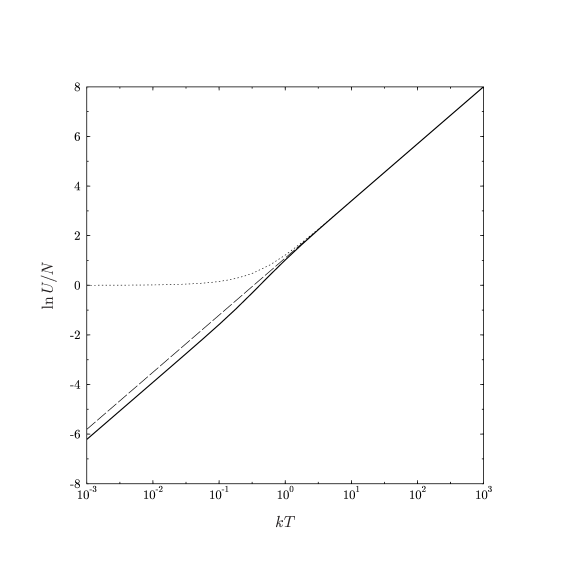
Figure 2: Average energy $U$ per particle of the ideal gas of bradyons (dotted line), luxons (dash line) and tachyons (solid line) given by equations (3.10), (3.13) and (3.14), respectively, where $u_{0}=1$, and $m=1$ in (3.10) and (3.14), as a function of $kT$ on a logarithmic scale. The parameters $u_{0}$ and $m$ are the same as in Fig. 1.

As an immediate application of the obtained relations (3.10), (3.13) and (3.14) we now write down the formulas on the specific heat per particle $C_{v}$ related to the average energy $U$ by

$$C_{v}=\frac{1}{N}\left(\frac{\partial U}{\partial T}\right)_{V}=-\frac{k\beta^{2}}{N}\left(\frac{\partial U}{\partial\beta}\right)_{V}.$$ (42)

Namely, we have for bradyons, luxons and tachyons, respectively

$$C_{vb}=k\left[3+(u_{0}\beta m)^{2}-3\frac{u_{0}\beta mK_{1}(u_{0}\beta m)}{K_{2}(u_{0}\beta m)}-\left(\frac{u_{0}\beta mK_{1}(u_{0}\beta m)}{K_{2}(u_{0}\beta m)}\right)^{2}\right],$$ (43)

$$C_{vl}=3k,$$ (44)

$$C_{vt}=k\left[3+\frac{u_{0}\beta mS_{-1,1}(u_{0}\beta m)-(u_{0}\beta m)^{2}S_{-2,0}(u_{0}\beta m)}{S_{0,2}(u_{0}\beta m)}-\left(\frac{u_{0}\beta mS_{-1,1}(u_{0}\beta m)}{S_{0,2}(u_{0}\beta m)}\right)^{2}\right].$$ (45)

The formula (3.20) can be written in an equivalent form

$$C_{vt}=-k\left[1+\frac{3[u_{0}\beta mS_{-1,3}(u_{0}\beta m)-5(u_{0}\beta m)^{2}S_{-2,4}(u_{0}\beta m)]}{S_{0,2}(u_{0}\beta m)}+\left(\frac{3u_{0}\beta mS_{-1,3}(u_{0}\beta m)}{S_{0,2}(u_{0}\beta m)}\right)^{2}\right],$$ (46)

following directly from (A.8). Up to some typo in 18 (3.21) coincides in the preferred frame, when $u_{0}=1$, with the formula originally obtained by Mrówczyński. We now return to (3.20). Taking into account (A.8) and (A.10) we obtain from (3.20) the following asymptotic relation:

$$C_{vt}=2k,\qquad u_{0}\beta m\gg 1.$$ (47)

In the case of bradyons we find

$$C_{vb}=\frac{3}{2}k,\qquad u_{0}\beta m\gg 1.$$ (48)

We remark that the asymptotic relations (3.22) and (3.23) can be formally obtained from (3.17), (3.16) and (3.11). Furthermore, it follows from numerical calculations that, in opposition to the case of bradyons when $C_{vb}$ is a decreasing function, the specific heat for tachyons has maximum (see Fig. 3). The occurence of the maximum was treated by Mrówczyński 18 as a formal property of $C_{vt}$. On the other hand, the maximum of the specific heat $C_{v}$ can be connected with the so called Schottky anomaly in a two-state system 19 . In the preferred frame, when $u_{0}=1$, the mass $m$ in the argument $u_{0}\beta m$ of the function $C_{vt}$ is a counterpart of the energy $E$ of a two-state system exhibiting Schottky anomaly, with a ground state of energy 0 and excited state of energy $E$. Although a physical interpretation of the maximum of the specific heat $C_{vt}$ is not clear, nevertheless, the experience with the Schottky anomaly shows that the knowledge of the abscissa of the maximum of the specific heat would enable determination of the tachyon mass $m$.

Figure 3: The plot of the specific heat of the ideal gas of bradyons (dotted line), luxons (dash line) and tachyons (solid line) given by (3.18), (3.19) and (3.20), respectively, where $u_{0}=1$ and $k=1$, versus $T/m$

We now discuss the entropy of the relativistic ideal gas. The Lorentz invariant entropy $S$ can be expressed in terms of the partition function and the average energy. Namely,

$$S=k\ln Z+\frac{U}{T}.$$ (49)

Using (3.24), (3.8) and the Stirling formula

$$N!\approx\left(\frac{N}{e}\right)^{N},$$ (50)

which holds for large $N$, we get

$$S=kN\ln Z_{1}-N\ln N+N+\frac{U}{T}.$$ (51)

From (3.26), (3.3) and (3.10) we obtain in the case of bradyons

$$S_{b}=kN\left(\ln\frac{4\pi Vm^{3}}{u_{0}N}+\ln\frac{K_{2}(u_{0}\beta m)}{u_{0}\beta m}+\frac{u_{0}\beta mK_{1}(u_{0}\beta m)}{K_{2}(u_{0}\beta m)}+4\right).$$ (52)

The formula on the entropy for the ideal gas of luxons such that

$$S_{l}=kN\left(\ln\frac{8\pi V}{u_{0}^{4}N\beta^{3}}+4\right)$$ (53)

is implied by (3.26), (3.5) and (3.13). Finally, using (3.26), (3.7) and (3.14) we find that the entropy of the ideal gas of tachyons can be written as

$$S_{t}=kN\left(\ln\frac{4\pi Vm^{3}}{u_{0}N}+\ln\frac{S_{0,2}(u_{0}\beta m)}{u_{0}\beta m}-\frac{u_{0}\beta mS_{-1,1}(u_{0}\beta m)}{S_{0,2}(u_{0}\beta m)}+4\right).$$ (54)

The dependence of the entropy of a relativistic ideal gas on the temperature is shown in Fig. 4. We remark that, as in the nonrelativistic case, the entropies (3.27), (3.28) and (3.29) approach minus infinity at the absolute zero. We recall that such behavior of the entropy means that the classical physics fails in the limit of very low temperatures and one should employ quantum statistical mechanics to calculate the entropy.

Figure 4: A semilogarithmic graph in which entropy per particle of the ideal gas of bradyons (dotted line), luxons (dash line) and tachyons (solid line) given by equations (3.27), (3.28) and (3.29), respectively, where $u_{0}=1$, $k=1$ and $m=1$, is plotted against the temperature.

Our purpose now is to study the Helmholtz free energy. The free energy $F$ is related to the partition function $Z$ by

$$F=-\frac{1}{\beta}\ln Z.$$ (55)

Using (3.30), (3.3), (3.5), (3.7) and the Stirling formula we obtain the following formulas on the free energy for bradyons, luxons and tachyons, respectively:

$$F_{b} = -\frac{N}{\beta}\left(\ln\frac{4\pi Vm^{3}}{u_{0}N}+\ln\frac{K_{2}(u_{0}\beta m)}{u_{0}\beta m}+1\right),$$ (56)

$$F_{l} = -\frac{N}{\beta}\left(\ln\frac{8\pi V}{u_{0}^{4}N\beta^{3}}+1\right),$$ (57)

$$F_{t} = -\frac{N}{\beta}\left(\ln\frac{4\pi Vm^{3}}{u_{0}N}+\ln\frac{S_{0,2}(u_{0}\beta m)}{u_{0}\beta m}+1\right).$$ (58)

As an immediate consequence of the above relations, and the formula on the chemical potential such that

$$\mu=\left(\frac{\partial F}{\partial N}\right)_{T,V}.$$ (59)

we get

$$\mu_{b} = -\frac{1}{\beta}\left(\ln\frac{4\pi Vm^{3}}{u_{0}N}+\ln\frac{K_{2}(u_{0}\beta m)}{u_{0}\beta m}\right),$$ (60)

$$\mu_{l} = -\frac{1}{\beta}\ln\frac{8\pi V}{u_{0}^{4}N\beta^{3}},$$ (61)

$$\mu_{t} = -\frac{1}{\beta}\left(\ln\frac{4\pi Vm^{3}}{u_{0}N}+\ln\frac{S_{0,2}(u_{0}\beta m)}{u_{0}\beta m}\right).$$ (62)

Now, making use of the formula on the pressure $p$ such that

$$p=-\left(\frac{\partial F}{\partial V}\right)_{T},$$ (63)

and the above formulas on the free energy we arrive at the equation of state which is the same for bradyons, luxons and tachyons, namely

$$pV=kTN.$$ (64)

Bearing in mind the formula (3.39) one may conclude, as for example Mrówczyński 18 , that “… all properties of the classical gas of tachyons and the gas of bradyons are similar and no new phenomena have been found in the case of tachyons”. We do not share such opinion. First of all it seems that the better version of the equation of state than (3.39) which does not distinguish bradyons, luxons and tachyons is the equation of state envolving the density of energy $U/V$ instead of the density of particles $N/V$ used in (3.39). Indeed, using (3.39), (3.10), (3.13) and (3.14) we get

$$p=\frac{\rho}{f_{b,l,t}(u_{0}\beta m)},$$ (65)

where $\rho=U/V$ is the density of energy and the functions $f_{b}$, $f_{l}$ and $f_{t}$ corresponding to the case of bradyons, luxons and tachyons, respectively, are given by

$$f_{b}(u_{0}\beta m) = 3+\frac{u_{0}\beta mK_{1}(u_{0}\beta m)}{K_{2}(u_{0}\beta m)},$$ (66)

$$f_{l}(u_{0}\beta m) = 3,$$ (67)

$$f_{t}(u_{0}\beta m) = 3-\frac{u_{0}\beta mS_{-1,1}(u_{0}\beta m)}{S_{0,2}(u_{0}\beta m)}.$$ (68)

The plot of the above functions is given in Fig. 5. We point out that in the high-temperature limit we have (see (3.12))

$$\lim_{(u_{0}\beta m)\to 0}f_{b,t}(u_{0}\beta m)=f_{l}(u_{0}\beta m)=3,$$ (69)

and in the limit $T\to 0$

$$f_{b}(u_{0}\beta m)=u_{0}\beta m,\qquad u_{0}\beta m\gg 1,$$ (70)

and

$$f_{t}(u_{0}\beta m)=2,\qquad u_{0}\beta m\gg 1,$$ (71)

following directly from (3.11) and (3.16), respectively.

Figure 5: The plot of the function $f_{b}$ (dotted line), $f_{l}$ (dash line) and $f_{t}$ (solid line) given by (3.37), (3.38) and (3.39), related to the equation of state (3.36) for bradyons, luxons and tachyons, respectively, where $u_{0}=1$, and $m=1$, in (3.37) and (3.39), versus $kT$.

Figure 6: A semilogarithmic graph in which squared velocity of particles of the ideal gas of bradyons given by (3.47), where $m=1$, is plotted against $kT$ on a logarithmic scale.

Figure 7: Average squared velocity of particles of the ideal gas of tachyons as a function of $kT$ (see 3.48) on a logarithmic scale. The parameter $m$ is the same as in Fig. 6.

Furthermore, in opposition to Mrówczyński, we treat the occurrence of the maximum of specific heat for tachyons as their important property distinguishing them from both bradyons and luxons. Even more evident difference of behavior of tachyons and bradyons is the dependence of velocity on the temperature. Indeed, it is clear in view of the fact that upon losing energy tachyon accelerate, that the velocity of a tachyon should be decreasing function of temperature. Of course, it is not the case for bradyons. To be more specific, consider the average squared velocity $\langle{\bm{v}}^{2}\rangle$. For the sake of simplicity we restrict to the preferred frame, i.e. we set $u_{0}=1$ and ${\bm{u}}={\bm{0}}$. The average squared velocity for bradyons is given by

$$\langle{\bm{v}}^{2}\rangle_{b}^{\rm PF}=\frac{V\int d^{3}\underline{\bm{p}}\,{\bm{v}}^{2}\exp\left(-\beta\sqrt{\underline{\bm{p}}^{2}+m^{2}}\right)}{Z_{1b}^{\rm PF}}=\frac{V\int d^{3}\underline{\bm{p}}\,\frac{\underline{\bm{p}}^{2}}{\underline{\bm{p}}^{2}+m^{2}}\exp\left(-\beta\sqrt{\underline{\bm{p}}^{2}+m^{2}}\right)}{Z_{1b}^{\rm PF}}\\ =\frac{m\beta\int_{1}^{\infty}x^{-1}(x^{2}-1)^{\frac{3}{2}}e^{-m\beta x}dx}{K_{2}(m\beta)},$$ (72)

where $Z_{1b}^{\rm PF}=Z_{1b|_{u_{0}=1}}$ (see (3.3)). The plot of $\langle{\bm{v}}^{2}\rangle_{b}^{\rm PF}$ versus $\beta$ is shown in Fig. 6. The average squared velocity for tachyons in the preferred frame can be written as (see Fig. 7)

$$\langle{\bm{v}}^{2}\rangle_{t}^{\rm PF}=\frac{V\int d^{3}\underline{\bm{p}}\,{\bm{v}}^{2}\exp\left(-\beta\sqrt{\underline{\bm{p}}^{2}-m^{2}}\right)}{Z_{1t}^{\rm PF}}=\frac{V\int d^{3}\underline{\bm{p}}\,\frac{\underline{\bm{p}}^{2}}{\underline{\bm{p}}^{2}-m^{2}}\exp\left(-\beta\sqrt{\underline{\bm{p}}^{2}-m^{2}}\right)}{Z_{1t}^{\rm PF}}\\ =\frac{m\beta\int_{0}^{\infty}x^{-1}(x^{2}+1)^{\frac{3}{2}}e^{-m\beta x}dx}{S_{0,2}(m\beta)},$$ (73)

where $Z_{1t}^{\rm PF}=Z_{1t|_{u_{0}=1}}$ (see (3.7)).

IV Quantum relativistic ideal gas

Our purpose now is to study the quantum ideal gas in the absolute synchronization. The classical formula (3.1) and the nonrelativistic relations in the case of the canonical ensamble 20 indicate the following form of the partition function for the relativistic gas of $N$ particles

$$Z_{N}=\sum_{n}\exp(-u_{0}^{2}\beta p^{0}_{n}),$$ (74)

where $p^{0}_{n}$ is the energy of the system in the state labelled by $n$. We recall that the grand canonical partition function is given by

$$\Xi=\sum_{N=1}^{\infty}s^{N}Z_{N},$$ (75)

where $s=e^{\beta\mu}$ is the fugacity and $\mu$ is the chemical potential. We point out that the product $\beta\mu$, and thus the fugacity, is Lorentz invariant (see (3.35), (3.36) and (3.37)). So the grand canonical partition function $\Xi$ is Lorentz invariant as well. As in the case of the classical ideal gas the average energy is related to the partition function by

$$U=-\frac{\partial}{\partial\beta}\ln\Xi.$$ (76)

Furthermore, we have also

$$\frac{pV}{kT}=\ln\Xi.$$ (77)

From (4.4) one can obtain the equation of the state by eliminating the parameter $s$ with the help of the relation

$$N=s\frac{\partial}{\partial s}\ln\Xi,$$ (78)

where $N$ is the average number of particles of the gas. Now taking into account the statistics of the particles and the form of (4.2) we obtain the following form of the grand canonical partition function:

$$\Xi=\prod_{\underline{\bm{p}}}(1\mp s\exp[-u_{0}^{2}\beta p^{0}(\underline{\bm{p}})])^{\mp 1},$$ (79)

where upper and lower sign refer to Bose-Einstein and Fermi-Dirac gases, respectively, and $p^{0}(\underline{\bm{p}})$ is given by (2.13), (2.14) and (2.15). Using (4.6) we arrive at the following form of the relations (4.3), (4.4) and (4.5):

$$U = u_{0}^{2}\sum_{\underline{\bm{p}}}\frac{p^{0}(\underline{\bm{p}})}{s^{-1}\exp[u_{0}^{2}\beta p^{0}(\underline{\bm{p}})]\mp 1},$$ (80)

$$\frac{pV}{kT} = \mp\sum_{\underline{\bm{p}}}\ln(1\mp s\exp[-u_{0}^{2}\beta p^{0}(\underline{\bm{p}})],$$ (81)

$$N = \sum_{\underline{\bm{p}}}\frac{1}{s^{-1}\exp[u_{0}^{2}\beta p^{0}(\underline{\bm{p}})]\mp 1}.$$ (82)

The above entities are well-defined for $s\geq 0$ in the case of fermions and $0\leq s\leq 1$ for bosons. In the limit $V\to\infty$ the sums (4.7), (4.8) and (4.9) change to integrals via the replacement 17

$$\sum_{\underline{\bm{p}}}\to\frac{V}{(2\pi)^{3}}\int d^{3}\underline{\bm{p}},$$ (83)

where we set $\hbar=1$. Hence, using (2.15), (2.16) and (2.17) we get

$$\left(\frac{U}{V}\right)_{b} = \frac{m^{4}}{2\pi^{2}}\int_{0}^{\infty}\frac{\cosh^{2}t\sinh^{2}t}{s^{-1}\exp(u_{0}\beta m\cosh t)\mp 1}dt$$ (84a)

$$= \frac{m^{2}}{2\pi^{2}u_{0}^{2}\beta^{2}}\sum_{n=1}^{\infty}\frac{(\pm 1)^{n+1}}{n^{2}}[3K_{2}(nu_{0}\beta m)+nu_{0}\beta mK_{1}(nu_{0}\beta m)]s^{n},$$ (84b)

$$\left(\frac{U}{V}\right)_{l}=\frac{u_{0}}{4\pi^{2}}\int_{-1}^{1}dx\sqrt{{\bm{u}}^{2}x^{2}+1}\int_{0}^{\infty}d|\underline{\bm{p}}|\frac{|\underline{\bm{p}}|^{3}}{s^{-1}\exp(u_{0}\beta\sqrt{{\bm{u}}^{2}x^{2}+1}|\underline{\bm{p}}|)\mp 1}$$ (85a)

$$=\frac{3}{\pi^{2}u_{0}^{4}\beta^{4}}\sum_{n=1}^{\infty}\frac{(\pm 1)^{n+1}}{n^{4}}s^{n},$$ (85b)

$$\left(\frac{U}{V}\right)_{t}=\frac{m^{4}}{2\pi^{2}}\int_{0}^{\infty}\frac{\cosh^{2}t\sinh^{2}t}{s^{-1}\exp(u_{0}\beta m\sinh t)\mp 1}dt$$ (86a)

$$=\frac{m^{2}}{2\pi^{2}u_{0}^{2}\beta^{2}}\sum_{n=1}^{\infty}\frac{(\pm 1)^{n+1}}{n^{2}}[3S_{0,2}(nu_{0}\beta m)-nu_{0}\beta mS_{-1,1}(nu_{0}\beta m)]s^{n}.$$ (86b)

We recall that the indices $b$, $l$, and $t$ refer to bradyons, luxons and tachyons, respectively. In the case of the Bose-Einstein gases we set $s<1$. The power series expansions (4.11b) and (4.13b) were obtained with the help of the basic properties of the Bessel functions and the Lommel functions presented in the Appendix. The expansion (4.12b) was derived with the use of the identity 21

$$\int_{0}^{\infty}\frac{x^{a-1}}{e^{bx}-c}=\frac{1}{cb^{a}}\Gamma(a)\sum_{n=1}^{\infty}\frac{c^{n}}{n^{a}},\qquad a>0,$$ (87)

where $\Gamma(x)$ is the gamma function. Furthermore, applying the same technique as with (4.11), (4.12) and (4.13) we find

$$\left(\frac{p}{kT}\right)_{b} = \mp\frac{m^{3}}{2\pi^{2}u_{0}}\int_{0}^{\infty}dt\sinh^{2}t\cosh t\ln[1\mp s\exp(-u_{0}\beta m\cosh t)]$$ (88a)

$$= \frac{m^{2}}{2\pi^{2}u_{0}^{2}\beta}\sum_{n=1}^{\infty}\frac{(\pm 1)^{n+1}}{n^{2}}K_{2}(nu_{0}\beta m)s^{n},$$ (88b)

$$\left(\frac{p}{kT}\right)_{l}=\frac{u_{0}\beta}{12\pi^{2}}\int_{-1}^{1}dx\sqrt{{\bm{u}}^{2}x^{2}+1}\int_{0}^{\infty}d|\underline{\bm{p}}|\frac{|\underline{\bm{p}}|^{3}}{s^{-1}\exp(u_{0}\beta\sqrt{{\bm{u}}^{2}x^{2}+1}\,|\underline{\bm{p}}|)\mp 1}$$ (89a)

$$=\frac{1}{\pi^{2}u_{0}^{4}\beta^{3}}\sum_{n=1}^{\infty}\frac{(\pm 1)^{n+1}}{n^{4}}s^{n},$$ (89b)

$$\left(\frac{p}{kT}\right)_{t} = \mp\frac{m^{3}}{2\pi^{2}u_{0}}\int_{0}^{\infty}dt\cosh^{2}t\sinh t\ln[1\mp s\exp(-u_{0}\beta m\sinh t)]$$ (90a)

$$= \frac{m^{2}}{2\pi^{2}u_{0}^{2}\beta}\sum_{n=1}^{\infty}\frac{(\pm 1)^{n+1}}{n^{2}}S_{0,2}(nu_{0}\beta m)s^{n}.$$ (90b)

Finally, we have

$$\left(\frac{N}{V}\right)_{b} = \frac{m^{3}}{2\pi^{2}u_{0}}\int_{0}^{\infty}\frac{\sinh^{2}t\cosh t}{s^{-1}\exp(u_{0}\beta m\cosh t)\mp 1}dt$$ (91a)

$$= \frac{m^{2}}{2\pi^{2}u_{0}^{2}\beta}\sum_{n=1}^{\infty}\frac{(\pm 1)^{n+1}}{n}K_{2}(nu_{0}\beta m)s^{n},$$ (91b)

$$\left(\frac{N}{V}\right)_{l}=\frac{1}{4\pi^{2}}\int_{-1}^{1}dx\int_{0}^{\infty}d|\underline{\bm{p}}|\frac{|\underline{\bm{p}}|^{2}}{s^{-1}\exp(u_{0}\beta\sqrt{{\bm{u}}^{2}x^{2}+1}\,|\underline{\bm{p}}|)\mp 1}$$ (92a)

$$=\frac{1}{\pi^{2}u_{0}^{4}\beta^{3}}\sum_{n=1}^{\infty}\frac{(\pm 1)^{n+1}}{n^{3}}s^{n},$$ (92b)

$$\left(\frac{N}{V}\right)_{t} = \frac{m^{3}}{2\pi^{2}u_{0}}\int_{0}^{\infty}\frac{\cosh^{2}t\sinh^{2}t}{s^{-1}\exp(u_{0}\beta m\sinh t)\mp 1}dt$$ (93a)

$$= \frac{m^{2}}{2\pi^{2}u_{0}^{2}\beta}\sum_{n=1}^{\infty}\frac{(\pm 1)^{n+1}}{n}S_{0,2}(nu_{0}\beta m)s^{n}.$$ (93b)

In the preferred frame, when $u_{0}=1$, the power series expansions for bradyons (4.11b), (4.15b) and (4.18b) reduce to the relations originally obtained by Glaser 22 . The expressions for tachyons (4.13b), (4.17b) and (4.20b) in the particular case of the preferred frame coincide up to a multiplicative normalization constant with the formulas originally derived by Mrówczyński 23 . We point out that an immediate consequence of (4.12b) and (4.16b) is the following relation

$$p=\frac{1}{3}\rho,$$ (94)

where $\rho=U/V$. Therefore the equation of state for the quantum ideal gas of massless particles has the same form as in the classical case described by (3.40) and (3.42).

IV.1 Classical limit

We now discuss the classical limit when $N/V\to 0$ and/or $T\to\infty$ that is $\beta\to 0$. In view of (4.18a), (4.19a) and (4.20a) it is clear that in this limit the fugacity $s$ is small as well. Therefore, we can approximate the series in the formulae (4.11)–(4.20) by the first terms linear in $s$. We find

$$\left(\frac{U}{V}\right)_{b} = \frac{m^{2}}{2\pi^{2}u_{0}^{2}\beta^{2}}[3K_{2}(u_{0}\beta m)+u_{0}\beta mK_{1}(u_{0}\beta m)]s,\qquad s\ll 1$$ (95)

$$\left(\frac{p}{kT}\right)_{b} = \frac{m^{2}}{2\pi^{2}u_{0}^{2}\beta}K_{2}(u_{0}\beta m)s,\qquad s\ll 1$$ (96)

$$\left(\frac{N}{V}\right)_{b} = \frac{m^{2}}{2\pi^{2}u_{0}^{2}\beta}K_{2}(u_{0}\beta m)s,\qquad s\ll 1.$$ (97)

From (4.23) and (4.24) we obtain the classical equation of state (see (3.39))

$$pV=kTN,\qquad s\ll 1.$$ (98)

We also have the relation following directly from (4.22) and (4.24)

$$\left(\frac{U}{N}\right)_{b}=\frac{1}{\beta}\left[3+u_{0}\beta m\frac{K_{1}(u_{0}\beta m)}{K_{2}(u_{0}\beta m)}\right],\qquad s\ll 1,$$ (99)

which is equivalent to the classical formula (3.10). Analogously, we have for luxons

$$\left(\frac{U}{V}\right)_{l} = \frac{3}{\pi^{2}u_{0}^{4}\beta^{4}}s,\qquad s\ll 1$$ (100)

$$\left(\frac{p}{kT}\right)_{l} = \frac{1}{\pi^{2}u_{0}^{4}\beta^{3}}s,\qquad s\ll 1$$ (101)

$$\left(\frac{N}{V}\right)_{l} = \frac{1}{\pi^{2}u_{0}^{4}\beta^{3}}s,\qquad s\ll 1.$$ (102)

As with bradyons we get from (4.28) and (4.29) the classical equation of state (4.25). On the other hand, (4.27) and (4.29) imply

$$\left(\frac{U}{N}\right)_{l}=\frac{3}{\beta},\qquad s\ll 1.$$ (103)

We have thus obtained the classical expression for the energy of the luxon ideal gas (3.13). Finally, consider the case of tachyons. The corresponding approximations can be written as

$$\left(\frac{U}{V}\right)_{t} = \frac{m^{2}}{2\pi^{2}u_{0}^{2}\beta^{2}}[3S_{0,2}(u_{0}\beta m)-u_{0}\beta mS_{-1,1}(u_{0}\beta m)]s,\qquad s\ll 1$$ (104)

$$\left(\frac{p}{kT}\right)_{t} = \frac{m^{2}}{2\pi^{2}u_{0}^{2}\beta}S_{0,2}(u_{0}\beta m)s,\qquad s\ll 1$$ (105)

$$\left(\frac{N}{V}\right)_{t} = \frac{m^{2}}{2\pi^{2}u_{0}^{2}\beta}S_{0,2}(u_{0}\beta m)s,\qquad s\ll 1.$$ (106)

As in the case of bradyons and luxons we obtain from (4.32) and (4.33) the classical equation of state (4.25). Furthermore, using (4.31) and (4.33) we get

$$\left(\frac{U}{N}\right)_{t}=\frac{1}{\beta}\left[3-u_{0}\beta m\frac{S_{-1,1}(u_{0}\beta m)}{S_{0,2}(u_{0}\beta m)}\right],\qquad s\ll 1,$$ (107)

coinciding with the classical expression (3.14).

IV.2 The limit $T\to 0$

Bearing in mind the technical complexity of calculations in the case of the degenerate Fermi-Dirac gas as well as the fact that only bosonic tachyons are admitted as a candidate for a dark matter we restrict to the Bose gas. Furthermore, in view of observations of 3 the limit $T\to 0$ in the case of Bose gas of bradyons is in fact the non-relativistic limit and will not be discussed herein. Consider the ideal gas of luxons. As in the special case of the photon gas which is well known to be degenerate for all temperatures, we set $s=1$. From (4.12), (4.16) and (4.19) we get

$$\frac{U}{V} = CT^{4},$$ (108)

$$p = \frac{1}{3}CT^{4},$$ (109)

$$N = aT^{3}V,$$ (110)

where $C=3\zeta(4)k^{4}/\pi^{2}u_{0}^{4}=\pi^{2}k^{4}/30u_{0}^{4}$, and $a=\zeta(3)k^{3}/\pi^{2}u_{0}^{4}$; $\zeta(x)=\sum_{n=1}^{\infty}\frac{1}{n^{x}}$ is the Riemann zeta function. In the case of the photon gas and the preferred frame ($u_{0}=1$), the constant $C$ and the constant $a$, taking into account the two polarization states of a photon, should be multiplied by 2, i.e. $C$ is then the Stefan-Boltzmann constant and $a=a_{\rm photon}$, respectively.

Now the entropy can be written as (see (3.24))

$$S=k\ln\Xi+\frac{U}{T}.$$ (111)

The equations (4.38), (4.4), (4.35) and (4.36) taken together yield

$$S=\frac{4}{3}VCT^{3}.$$ (112)

As expected, the entropy vanishes at zero temperature. The formula (4.39) can be also obtained from the well-known relation

$$S=\int_{0}^{T}\frac{C_{V}}{T}dT,$$ (113)

where

$$C_{V}=\left(\frac{\partial U}{\partial T}\right)_{V}=4CVT^{3},$$ (114)

following directly from (4.35).

We now study the Bose gas of tachyons in the low-temperature limit. In this limit one cannot simply replace sums (4.7), (4.8) and (4.9) by integrals because when $s\simeq 1$ the terms referring to the ground state can give finite contributions to series. Therefore, we separate the sum (4.9) into two contributions — the number of particles in the ground state $N_{0}$ and the number of particles in the excited states 20 . Using (4.20b) we find

$$N=N_{0}+V\frac{m^{2}}{2\pi^{2}u_{0}^{2}\beta}\sum_{n=1}^{\infty}\frac{1}{n}S_{0,2}(nu_{0}\beta m)s^{n},$$ (115)

where

$$N_{0}=\frac{1}{s^{-1}-1}.$$ (116)

We recall that the accumulation of bosons in the ground states is known as Bose-Einstein condensation. Taking the limit of the strong degeneration $s=1$ and utilizing for $T\to 0$, that is $\beta\to\infty$, the asymptotic formula (A.10) we obtain from (4.42) the relation

$$N=N_{0}+V\frac{m}{2\pi^{2}u_{0}^{3}\beta^{2}}\zeta(2)=N_{0}+V\frac{mk^{2}}{12u_{0}^{3}}T^{2}.$$ (117)

From (4.44) it follows that the Bose-Einstein condensation occurs at temperatures lower than the critical one given by

$$T_{c}=\sqrt{\frac{12Nu_{0}^{3}}{Vmk^{2}}},$$ (118)

and densities higher than the critical density such that

$$d_{c}=\frac{mk^{2}}{12u_{0}^{3}}T^{2}.$$ (119)

Furthermore, using (4.44) and (4.45) we get

$$\frac{N_{0}}{N}=\left[1-\left(\frac{T}{T_{c}}\right)^{2}\right],\qquad T\leq T_{c}.$$ (120)

For temperatures greater than $T_{c}$ but close enough to $T_{c}$ to enable setting $s=1$, we have

$$\frac{U}{V} = \frac{m}{\pi^{2}u_{0}^{3}\beta^{3}}\zeta(3),$$ (121)

$$\frac{p}{kT} = \frac{m}{2\pi^{2}u_{0}^{3}\beta^{2}}\zeta(3),$$ (122)

$$\frac{N}{V} = \frac{m}{2\pi^{2}u_{0}^{3}\beta^{2}}\zeta(2).$$ (123)

Hence, taking into account (4.49) and (4.50) we arrive at the equation of state of the form

$$pV=\frac{\zeta(3)}{\zeta(2)}NkT,\qquad T\gtrsim T_{c}.$$ (124)

Using (4.48) and (4.50) we also obtain

$$U=2\frac{\zeta(3)}{\zeta(2)}NkT,\qquad T\gtrsim T_{c}.$$ (125)

Therefore the specific heat is

$$C_{V}=2\frac{\zeta(3)}{\zeta(2)}Nk,\qquad T\gtrsim T_{c}.$$ (126)

For temperatures lower than $T_{c}$ one should use $N-N_{0}$ instead of $N$. Therefore the equation of state takes the form

$$p=\frac{m}{2\pi^{2}u_{0}^{3}}\zeta(3)k^{3}T^{3},\qquad T\leq T_{c},$$ (127)

and (4.52) is replaced by

$$U=\frac{m}{\pi^{2}u_{0}^{3}}\zeta(3)k^{3}T^{3}V,\qquad T\leq T_{c}.$$ (128)

Using (4.38), (4.4), (4.54) and (4.55) we obtain the following formula on the entropy:

$$S=\frac{3m}{2\pi^{2}u_{0}^{3}}V\zeta(3)k^{3}T^{2},\qquad T\leq T_{c},$$ (129)

implying vanishing of the entropy at zero temperature. The relation (4.56) is also a consequence of (4.40) and the expression on the specific heat such that

$$C_{V}=\frac{3m}{\pi^{2}u_{0}^{3}}V\zeta(3)k^{3}T^{2},\qquad T\leq T_{c},$$ (130)

following immediately from (4.55). The discussion of the relations satisfied by the thermodynamic functions for the non-relativistic Bose gas in the case of $T\gtrsim T_{c}$, and $T\leq T_{c}$ can be found in the book 24 .

V Conclusions

In this work we have derived the Lorentz covariant form of thermodynamic functions for the relativistic ideal gas in both classical and quantum cases. We stress that the applied approach based on the concept of the preferred frame is the only one which enables formulation of covariant statistical mechanics of tachyons. On the other hand, an advantage of the formalism introduced in this paper is that it allows to study from the unique point of view all kinds of relativistic gases including bradyon, luxon, and tachyon ones. Bearing in mind the possible applications of the observations of this work we point out the specific heat of the tachyon gas showing behavior analogous to Schottky anomaly (see Fig. 3), and the formula (4.43) on the critical temperature for the Bose condensation which seem to be of importance for the determination of the mass of a tachyon. The results obtained in this paper can be also helpful in discussion of the dark matter and dark energy in astrophysics and cosmology. Indeed, the observations of stars motion in galactics, galactic clusters, cluster masses as inferred from gravitational lensing strongly suggest existence of an exotic dark matter component of the universe. Moreover, from observations of supernova IA populations we know that the universe accelerates which demands existence of exotic dark energy. A possible attempts to explanation of the exotic content of the universe need some radical extension of standard physics. One of candidates is tachyonic fluid (see for example 26 ) or the rolling tachyon field 9 ; 27 .

Appendix A

We first recall some properties of the modified Bessel functions (Macdonald functions) $K_{\nu}(x)$. These functions have the integral representation of the form

$$K_{\nu}(x)=\int_{0}^{\infty}e^{-x\cosh t}\cosh\nu t\,dt,\qquad x>0.$$ (131)

They satisfy the following recurrence relations:

$$K^{\prime}_{\nu}(x)=\frac{\nu}{x}K_{\nu}(x)-K_{\nu+1}(x)=-\frac{\nu}{x}K_{\nu}(x)-K_{\nu-1}(x),$$ (132)

where prime designates differentiation. We have the asymptotic formulas

$$K_{n}(x) = \frac{1}{2}(n-1)!\left(\frac{2}{x}\right)^{n},\qquad x\ll 1,$$ (133)

$$K_{\nu}(x) = \sqrt{\frac{\pi}{2x}}e^{-x},\qquad x\gg 1.$$ (134)

We now briefly sketch the basic properties of the Lommel functions $S_{\mu,\nu}(x)$ 21 ; 25 . The Lommel functions $S_{0,\nu}(x)$ are given by

$$S_{0,\nu}(x)=\int_{0}^{\infty}e^{-x\sinh t}\cosh\nu t\,dt=\frac{x}{\nu}\int_{0}^{\infty}e^{-x\sinh t}\cosh t\sinh\nu t\,dt,\qquad x>0.$$ (135)

The Lommel functions $S_{\nu,\nu}(x)$ can be expressed in terms of the Struve functions ${\bf H}_{\nu}(x)$ and the Bessel functions $Y_{\nu}(x)$ (Neumann functions) also designated by $N_{\nu}(x)$. We have

$$S_{\nu,\nu}(x)=2^{\nu-1}\sqrt{\pi}\Gamma(\nu+\hbox{$\scriptstyle 1\over 2$})[{\bf H}_{\nu}(x)-Y_{\nu}(x)].$$ (136)

The recurrence relations for $S_{\mu,\nu}(x)$ are of the form

$$S_{\mu+2,\nu}(x)=x^{\mu+1}-[(\mu+1)^{2}-\nu^{2}]S_{\mu,\nu}(x),$$ (137)

$$S^{\prime}_{\mu,\nu}(x)=\frac{\nu}{x}S_{\mu,\nu}(x)+(\mu-\nu-1)S_{\mu-1,\nu+1}(x)=-\frac{\nu}{x}S_{\mu,\nu}(x)+(\mu+\nu-1)S_{\mu-1,\nu-1}(x).$$ (138)

For small and large argument $S_{0,2}(x)$ can be approximated as

$$S_{0,2}(x) = \frac{2}{x^{2}},\qquad x\ll 1,$$ (139)

$$S_{0,2}(x) = \frac{1}{x},\qquad x\gg 1.$$ (140)

We remark that $S_{0,2}(x)$ and $K_{2}(x)$ are approximated by the same function in the limit $x\ll 1$.

References

• (1) F. Jüttner, Ann. Phys. 34, 856 (1911); 35, 145 (1911).
• (2) D. Ter Haar, H. Wergeland, Phys. Rep. 1, 31 (1971).
• (3) C. Aragão de Carvalho and S. Goulart Rosa Jr, J. Phys. A 13, 3233 (1980).
• (4) J. Rembieliński, K.A. Smoliński and G. Duniec, Found. Phys. Lett. 14, 487 (2001).
• (5) J. Rembieliński, Internat. J. Modern Phys. A 12, 1677 (1997).
• (6) G. Feinberg, Phys. Rev. 159, 1089 (1967).
• (7) P.C.W. Davies, Internat. J. Theoret. Phys. 43, 141 (2004); A. Das et al, Phys. Rev. D 72, 043528 (2005).
• (8) J.S. Bagla, H.K. Jassal and T. Padmanabhan, Phys. Rev. D 67, 063504 (2003); E.J. Copeland et al, Phys. Rev. D 71, 043003 (2005); A. Das et al, Phys. Rev. D 72, 043528 (2005); E. Calcagni and A.R. Liddle, Phys. Rev. D 74, 043528 (2006).
• (9) S. Mukohyama, Phys. Rev. D 66, 024009 (2002).
• (10) F.A.E. Pirani, Phys. Rev. D 1, 3224 (1970); J.K. Kowalczyński, Internat. J. Theoret. Phys. 23, 27 (1984).
• (11) E.C.G. Sudarshan, in: E. Recami ed., Tachyons, Monopoles and Related Topics (North-Holland, New York, 1978), pp. 43–46.
• (12) K. Kamoi and S. Kamefuchi, in: E. Recami ed., Tachyons, Monopoles and Related Topics (North-Holland, New York, 1978), pp. 159–167.
• (13) J. Rembieliński, Phys. Lett. A 78, 33 (1980).
• (14) P. Caban and J. Rembieliński, Phys. Rev. A 59, 4187 (1999).
• (15) G. Amelino-Camelia, Internat. J. Modern Phys. D 11, 35 (2002); J. Magueijo and L. Smolin, Phys. Rev. D 67, 044017 (2003).
• (16) T. Jacobson and D. Mattingly, Phys. Rev. D 64, 024028 (2001).
• (17) D. Colladay and V.A. Kostelecký, Phys. Rev. D 55, 6760 (1997); ibid Phys. Rev. D 58, 116002 (1998); V.A. Kostelecký, Phys. Rev. D 69, 105009 (2004).
• (18) S. Mrówczyński, Lett. Nuovo Cim. 38, 247 (1983).
• (19) H.B. Callen, Thermodynamics and an Introduction to Thermostatics (Wiley, New York, 1985).
• (20) K. Huang, Statistical Mechanics (Wiley, New York, 1987).
• (21) I.S. Gradshteyn and I.M. Ryzhik, Tables of Integrals, Series, and Products (Academic Press, New York, 2000).
• (22) W. Glaser, Z. Phys. 94, 677 (1935).
• (23) S. Mrówczyński, Nuovo Cim. B 81, 179 (1984).
• (24) J. Łopuszański and A. Pawlikowski, Statistical Physics (PWN, Warsaw, 1969).
• (25) H. Bateman, Higher Transcendental Functions, vol. 2, (McGraw-Hill, New York, 1953).
• (26) P.C.W. Davies, Internat. J. Theoret. Phys. 43, 141 (2004).
• (27) G. Gibbons, Classical Quantum Gravity 20, 5231 (2003).