Dynamical Simulations of Magnetically Channeled Line-Driven Stellar Winds:
II. The Effects of Field-Aligned Rotation

Abstract

Building upon our previous MHD simulation study of magnetic channeling in radiatively driven stellar winds, we examine here the additional dynamical effects of stellar rotation in the (still) 2-D axisymmetric case of an aligned dipole surface field. In addition to the magnetic confinement parameter $\eta_{\ast}$ introduced in Paper I, we characterize the stellar rotation in terms of a parameter $W\equiv V_{\rm{rot}}/V_{\rm{orb}}$ (the ratio of the equatorial surface rotation speed to orbital speed), examining specifically models with moderately strong rotation $W=$ 0.25 and 0.5, and comparing these to analogous non-rotating cases. Defining the associated Alfvén radius $R_{\rm{A}}\approx\eta_{\ast}^{1/4}R_{\ast}$ and Kepler corotation radius $R_{\rm{K}}\approx W^{-2/3}R_{\ast}$, we find rotation effects are weak for models with $R_{\rm{A}}<R_{\rm{K}}$, but can be substantial and even dominant for models with $R_{\rm{A}}\mathrel{\hbox to0.0pt{\lower 3.0pt\hbox{$\mathchar 536\relax$}\hss}\raise 2.0pt\hbox{$\mathchar 318\relax$}}R_{\rm{K}}$. In particular, by extending our simulations to magnetic confinement parameters (up to $\eta_{\ast}=1000$) that are well above those ($\eta_{\ast}=10$) considered in Paper I, we are able to study cases with $R_{\rm{A}}\gg R_{\rm{K}}$; we find that these do indeed show clear formation of the rigid-body disk predicted in previous analytic models, with however a rather complex, dynamic behavior characterized by both episodes of downward infall and outward breakout that limit the buildup of disk mass. Overall, the results provide an intriguing glimpse into the complex interplay between rotation and magnetic confinement, and form the basis for a full MHD description of the rigid-body disks expected in strongly magnetic Bp stars like $\sigma$ Ori E.

1 INTRODUCTION

In Paper I of this series (ud-Doula & Owocki, 2002), we examined the effect of a large-scale dipole magnetic field on the radiatively driven wind from a hot, massive star. The radiative envelopes of such hot stars means they lack the strong convection zone that drives the dynamo generation of magnetic activity cycles in the Sun and other relatively cool stars. Nonetheless, in recent years spectro-polarimetric observations have led to positive detections of large-scale fields in several such hot stars, often well fit by a dipole tilted relative to the star’s rotation axis (e.g., Donati et al. 2002). In some cases the associated period of rotational modulation is quite long, weeks or even years (e.g. in $\theta^{1}$ Ori C, HD191612; Donati et al. 2006), implying that the direct dynamical effect of rotation on the magnetic channeling of the wind is likely to be limited. As a first approximation, the MHD simulation models of Paper I thus ignored the effects of rotation.

More generally, however, massive stars tend to have quite rapid rotation, as evidenced both by the substantial broadening in photospheric spectral lines (Conti & Ebbets, 1977; Fukuda, 1982), which indicate projected rotation speeds of hundreds of km/s, and by the relatively short-period of observed modulations for some stars, e.g. the magnetic Bp star $\sigma$ Ori E, for which the inferred rotation period is about 1.2 d (Walborn, 1981). Both lines of evidence suggest that hot-star rotation rates are commonly a substantial fraction of the ‘critical’ rate at which the equatorial surface would be in Keplerian orbit. Since this implies centrifugal forces that are comparable to the inward pull of gravity, it is clear that such levels of rotation could significantly influence the magnetic channeling of a stellar wind.

Previous studies have focused in particular on the potential role of magnetic fields in spinning up the wind outflow and channeling it into an equatorial disk that might be centrifugally supported against gravity. Cassinelli et al. (2002) argued that such magnetic spin-up could effectively eject material into a “Magnetically Torqued Disk” (MTD), in which individual fluid elements would be in local Keplerian orbit, and specifically proposed this as a model for the Keplerian “decretion disks” inferred for Be stars. For the chemically peculiar Bp stars that have been directly observed to have very strong magnetic fields ($\mathrel{\hbox to0.0pt{\lower 3.0pt\hbox{$\mathchar 536\relax$}\hss}\raise 2.0pt\hbox{$\mathchar 318\relax$}}10^{4}$ G), Townsend & Owocki (2005, herefter TO-05) developed a somewhat different “Rigidly Rotating Magnetosphere” (RRM) paradigm in which the field again spins up and channels wind material into a disk, but now is also sufficiently strong to hold it in rigid body rotation. This RRM model has proven particularly successful in explaining the rotationally modulated Balmer emission observed from $\sigma$ Ori E (Townsend, Owocki & Groote, 2005).

To test these semi-analytic paradigms, we have made some initial efforts to extend the numerical MHD simulations of Paper I to include rotation in the simple 2D axisymmetric case of a rotation-aligned dipole. The results indicate that a large-scale field strong enough to torque wind material to Keplerian orbital speed tends also to propel material away from the star, rather than into the kind of stationary, Keplerian disk envisioned in the MTD model (ud-Doula, Townsend & Owocki, 2006; Owocki, Townsend & ud-Doula, 2006a, b). However, for cases with strong-enough magnetic confinement to hold material down against such outward escape, there can indeed form a limited rigid-body disk quite similar to that predicted by the RRM model (Owocki & ud-Doula, 2003; Owocki, 2006). But even in such cases, there is irregular breakout of material from the outer disk, leading to a sudden magnetic reconnection heating that could explain the hard X-ray flares seen from $\sigma$ Ori E (ud-Doula et al., 2006).

The present paper further extends these previous MHD simulations with a more extensive 2-D parameter study covering models over a range in both rotation rate and degree of magnetic confinement. A particular focus is to develop a clearer physical picture of the complex competition between wind-fed build-up of material in a disk vs. losses by both outward ejection and infall back to the star. Moreover, the broad parameter study here allows us to examine in detail how these processes are affected by various combinations of rotation rate and magnetic field strength. To lay the basis for the results presented in section 4, section 2 first reviews the general numerical MHD approach, and section 3 defines the overall parameter domain. Section 5 concludes with a summary and outline for future work.

2 NUMERICAL METHOD

2.1 Vector form of basic MHD equations

As in Paper I, our general approach is to use the ZEUS-3D (Stone & Norman, 1992) numerical MHD code to evolve a consistent dynamical solution for a line-driven stellar wind from a star with a dipole surface field. Our implementation here again adopts spherical polar coordinates with radius $r$, co-latitude $\theta$, and azimuth $\phi$, but now in a “2.5-D” formulation that allows for non-zero azimuthal components of both the magnetic field $B_{\phi}$ and velocity $v_{\phi}$, while still assuming all quantities are constant in the azimuthal coordinate angle $\phi$. To maintain this 2.5-D axisymmetry, we assume the stellar magnetic field to be a pure-dipole with polar axis aligned with the rotation axis of the star.

In vector form, the standard formulation of magnetohydrodynamics includes equations for mass continuity,

$$\frac{\partial\rho}{\partial t}+{\bf v}\cdot\nabla\rho+\rho\nabla\cdot{\bf v}=0\,,$$ (1)

and momentum balance,

$$\frac{\partial{\bf v}}{\partial t}+{\bf v}\cdot\nabla{\bf v}=-\frac{\nabla p}{\rho}+\frac{1}{4\pi\rho}(\nabla\times{\bf B})\times{\bf B}-{GM{\hat{\bf r}}\over r^{2}}+{\bf g}_{\rm{lines}},$$ (2)

where the notation follows common conventions, and is defined in detail in section 2 of Paper I. (Note that eqn. (2) here corrects some minor errors in the corresponding eqn. (2) of Paper I.)

2.2 Rotation terms in the advective acceleration

The inclusion of a finite rotation in the present work leads to additional nonzero terms proportional to the azimuthal velocity $v_{\phi}$ within the three vector components of the advective acceleration,

$$\left[{\bf v}\cdot\nabla{\bf v}\right]_{r}={v_{r}}\,{\partial v_{r}\over\partial r}~{}+~{}{v_{\theta}\over r}\,{\partial v_{r}\over\partial\theta}-{v_{\theta}^{2}+v_{\phi}^{2}\over r}\,,$$ (3)

$$\left[{\bf v}\cdot\nabla{\bf v}\right]_{\theta}={v_{r}}\,{\partial v_{\theta}\over\partial r}~{}+~{}{v_{\theta}\over r}\,{\partial v_{\theta}\over\partial\theta}-\cot\theta\,{v_{\phi}^{2}\over r}~{}+~{}{v_{r}v_{\theta}\over r}\,,$$ (4)

$$\left[{\bf v}\cdot\nabla{\bf v}\right]_{\phi}={v_{r}}\,{\partial v_{\phi}\over\partial r}~{}+~{}{v_{\theta}\over r}\,{\partial v_{\phi}\over\partial\theta}~{}+~{}\cot\theta\,{v_{\phi}v_{\theta}\over r}~{}+~{}{v_{\phi}v_{r}\over r}\,.$$ (5)

The terms here without derivatives represent the inertial forces arising from the curvature of the coordinate system, namely centrifugal and coriolis forces, which, e.g., in the absence of external torques, enforce conservation of angular momentum within the rotating flow described in spherical coordinates.

Of course, in magnetic models the Lorentz force, represented by the second term on the right side of eqn. (2), can significantly channel the flow, competing against these inertial terms. In rotating models, this Lorentz force can now also impart a significant torque to spin up the outflow; moreover it now includes additional terms proportional to the non-zero $B_{\phi}$, which themselves represent a component for outward angular momentum transport.

This competition between the magnetic Lorentz force and the inertia terms associated with rotation represents a central focus of the present study. In some ways, it parallels the central competition examined in Paper 1, namely between magnetic forces and the inertia associated with the radial outflow of the wind.

2.3 Radial driving of wind outflow

This radial outflow arises from the strong radial driving of the line-force, $\bf{g}_{\rm{lines}}$. As in Paper I, we model this here in terms of the standard Castor, Abbott & Klein (1975, hereafter CAK) formalism, corrected for the finite cone angle of the star, using a spherical expansion approximation for the local flow gradients (Pauldrach, Puls, Hummer & Kudritzki, 1985; Friend & Abbott, 1986) and ignoring non-radial line-force components that can arise in a non-spherical outflow. Although such non-radial terms are typically only a few percent of the radial force, in non-magnetic models of rotating winds, they act without much competition in the lateral force balance, and so can have surprisingly strong effects on the wind channeling and rotation (Owocki, Cranmer & Gayley, 1996; Gayley & Owocki, 2000). But in magnetic models with an already strong component of non-radial force, such terms are not very significant, and since their full inclusion substantially complicates both the numerical computation and the analysis of simulation results, we have elected to defer further consideration of such non-radial line-force terms to future studies.

By limiting our study to moderately fast rotation, half or less of the critical rate, we are also able to neglect the effects of stellar oblateness and gravity darkening.

2.4 Isothermal flow approximation

Another simplification retained from Paper I is that the flow is strictly isothermal. This is generally a reasonable approximation in steady-state, spherical wind models, wherein the competition between photoionization heating and radiative cooling keeps the wind close to the stellar effective temperature (Pauldrach, 1987; Drew, 1989). However, models with significant magnetic channeling can guide the flow toward strong shock compressions that heat the gas to temperatures of millions of Kelvin. The associated extensive X-ray emission (Babel & Montmerle, 1997a, b) has indeed been a focus of some our previous simulations aimed at modeling the observed X-ray spectrum from $\theta^{1}$ Ori C (Gagné et al., 2005). Moreover, our other simulations show that reconnection heating associated with centrifugally driven breakout events might provide a basis for explaining the relatively hard X-ray flare events seen in the magnetic B-star $\sigma$ Ori E (ud-Doula et al., 2006).

While such detailed treatments of the wind energy balance can thus be quite important for modeling the X-ray emission from specific stars, including this in the general parameter study here would require introducing an additional free parameter, associated with the wind density, and representing the relative importance of radiative cooling in the post-shock region (ud-Doula, 2003). This would in effect require a three-dimensional parameter study, representing cooling, magnetic confinement, and rotation. To maintain the focus here on just the one additional degree of freedom associated with rotation, built upon the study of isothermal magnetic confinement in Paper I, we again assume a simple isothermal wind with the wind temperature kept equal to the stellar effective temperature, here taken to be 50,000 K.

A further advantage is that, at such a temperature, the gas pressure terms in eqn. (2) are typically unimportant throughout most of the supersonic outflow. Thus, although these pressure terms are still fully included in the numerical simulations, they can be largely ignored in interpretation of results, allowing for a focus on the dominant competing forces associated with gravity, radiative driving, magnetic field and flow inertia.

2.5 Boundary conditions and numerical considerations

Finally, numerical specifications such as the computational grid and boundary conditions are again similar to Paper I, except of course that the lower boundary now has a non-zero azimuthal speed $v_{\phi}(R_{\ast},\theta)=V_{\rm{rot}}\sin\theta$, where $V_{\rm{rot}}$ is the equatorial surface rotation speed. Also, instead of setting the azimuthal field to zero at the stellar surface, as in Paper I, we now compute a generally non-zero $B_{\phi}$ at the lower boundary ghost-zone by linear extrapolation from the values in the two innermost zones of the actual computational grid. This assumes vanishing second derivatives of the azimuthal field components.

In all simulations presented here the time step is based on relatively low Courant number of 0.3, a choice that helps ensure stability and reduced error in computed shock properties (Falle, 2002). Simulations of selected models with an even lower Courant number of 0.1 gave very similar results to the standard runs.

3 TWO-PARAMETER STUDY

3.1 Magnetic confinement parameter $\eta_{\ast}$

Let us now consider how best to frame our parameter study for the combined effects of rotation and magnetic channeling in a line-driven wind. In the absence of significant rotation or magnetic fields, the line-force overcomes the stellar gravity to drive a nearly radial wind outflow characterized by a mass loss rate ${\dot{M}}$ and terminal wind speed $V_{\infty}$. When a magnetic field is added, the inertia of this radial outflow competes against the Lorentz forces. A key result of Paper I is that the overall net effect of a magnetic field in diverting such a wind outflow can be characterized by a single magnetic confinement parameter,

$$\eta_{\ast}\equiv\frac{B_{eq}^{2}\,R_{\ast}^{2}}{\dot{M}\,V_{\infty}}\,,$$ (6)

where $B_{eq}$ is the surface field strength at the magnetic equator. This sets the scale of the ratio of magnetic energy to wind kinetic energy,

$$\eta(r)\equiv\frac{B^{2}/8\pi}{\rho v^{2}/2}=\eta_{\ast}\,\left[\frac{(r/R_{\ast})^{2-2q}}{(1-R_{\ast}/r)^{\beta}}\right]=\left(\frac{V_{A}}{v}\right)^{2}=M_{A}^{-2}\,.$$ (7)

The last two equalities emphasize this energy ratio can also be cast as the square of the ratio of the Alfvén speed, $V_{A}\equiv B/\sqrt{4\pi\rho}$, to flow speed, $v$, i.e. as the inverse square of the Alfvénic Mach number, $M_{A}\equiv v/V_{A}$.

The square bracket factor in the middle equality shows the overall radial variation; $q$ is the power-law exponent for radial decline of the assumed stellar field, e.g. $q=3$ for a pure dipole, and $\beta$ is the velocity-law index, with typically $\beta\approx 1$. For a star with a non-zero field, we have $\eta_{\ast}>0$, and so given the vanishing of the flow speed at the atmospheric wind base, this energy ratio always starts as a large number near the stellar surface, $\eta(r\rightarrow R_{\ast})\rightarrow\infty$. But from there outward it declines quite steeply, asymptotically as $r^{-4}$ for a dipole, crossing unity at the Alfvén radius defined implicitly by $\eta(R_{A})\equiv 1$.

For a canonical $\beta=1$ wind velocity law, explicit solution for $R_{\rm{A}}$ along the magnetic equator requires finding the appropriate root of

$$\left({R_{A}\over R_{\ast}}\right)^{2q-2}-\left({R_{A}\over R_{\ast}}\right)^{2q-3}=\eta_{\ast}\,,$$ (8)

which for integer $2q$ is just a simple polynomial, specifically a quadratic, cubic, or quartic for $q=$ 2, 2.5, or 3. Even for non-integer values of $2q$, the relevant solutions can be approximated (via numerical fitting) to within a few percent by the simple general expression,

$$\frac{R_{\rm{A}}}{R_{\ast}}\approx 1+(\eta_{\ast}+1/4)^{1/(2q-2)}-(1/4)^{1/(2q-2)}\,.$$ (9)

For weak confinement, $\eta_{\ast}\ll 1$, we find $R_{\rm{A}}\rightarrow R_{\ast}$, while for strong confinement, $\eta_{\ast}\gg 1$, we obtain $R_{\rm{A}}\rightarrow\eta_{\ast}^{1/(2q-2)}R_{\ast}$. In particular, for the standard dipole case with $q=3$, we expect the strong-confinement scaling $R_{\rm{A}}/R_{\ast}\approx 0.3+\eta_{\ast}^{1/4}$.

Clearly $R_{\rm{A}}$ represents the radius at which the wind speed $v$ exceeds the local Alfvén speed $V_{A}$. But Paper I showed that it also characterizes the maximum radius where the magnetic field still dominates over the wind, and is just somewhat above (i.e., by 20-30%) the maximum extent of closed loops in the magnetosphere. Moreover, as we shall see below, in rotating winds these closed loop regions tend to co-rotate nearly rigidly with the underlying star, and in this sense $R_{\rm{A}}$ is just above the maximum radius for wind co-rotation near the equator. For convenience in discussing results, let us thus denote the maximum radius of such closed (and generally co-rotating) loops as

$$R_{\rm{c}}\approx R_{\ast}+0.7(R_{\rm{A}}-R_{\ast})\,.$$ (10)

3.2 Rotation parameter $W$

Let us next seek a similarly convenient parameterization for the stellar rotation. This can again be characterized in terms of a speed, namely the equatorial surface rotation speed $V_{\rm{rot}}$. But instead of relating that to the flow speed or Alfvén speed in the stellar wind, the stellar origin of rotation suggests it may be better to compare it to a speed representative of the gravity at the stellar surface. Specifically, let us thus define our dimensionless rotation parameter as

$$W\equiv\frac{V_{\rm{rot}}}{V_{\rm{orb}}}\,,$$ (11)

where $V_{\rm{orb}}\equiv\sqrt{GM/R_{\ast}}$ is the orbital speed near the equatorial surface. This characterizes the azimuthal speed needed for the outward centrifugal forces to balance the stellar surface gravity. It is only a factor $1/\sqrt{2}$ less than the speed $V_{\rm{esc}}$ needed to fully escape the star’s surface gravitational potential.

For a non-magnetic rotating star, conservation of angular momentum in a wind outflow causes the azimuthal speed near the equator to decline outward as $v_{\phi}\sim 1/r$, meaning that rotation effects tend to be of diminishing importance in the outer wind.

By contrast, in a rotating star with a sufficiently strong magnetic field, magnetic torques on the wind can spin it up; for some region near the star, i.e., up to about the maximum loop closure radius $R_{\rm{c}}$, they can even maintain a nearly rigid-body rotation, for which the azimuthal speed now increases outward in proportion to the radius,

$$v_{\phi}(r)=V_{\rm{rot}}\,\frac{r}{R_{\ast}}~{}~{};~{}~{}r\mathrel{\hbox to0.0pt{\lower 3.0pt\hbox{$\mathchar 536\relax$}\hss}\raise 2.0pt\hbox{$\mathchar 316\relax$}}R_{\rm{c}}\,.$$ (12)

As such, even for a star with surface rotation below the orbital speed, $W<1$, maintaining rigid rotation will eventually lead to a balance between the outward centrifugal force from rotation and the inward force of gravity,

$$\frac{v_{\phi}^{2}(R_{\rm{K}})}{R_{\rm{K}}}=\frac{GM}{R_{\rm{K}}^{2}}\,.$$ (13)

Combining this with eqns. (11) and (12) gives a simple expression for the associated “Kepler radius”,

$$R_{\rm{K}}=W^{-2/3}R_{\ast}\,.$$ (14)

Unsupported material at radii $r<R_{\rm{K}}$ will tend to fall back toward the star, but any material maintained in rigid-rotation to radii $r>R_{\rm{K}}$ will have a centrifugal force that exceeds gravity, and so will tend to be propelled further outward. Indeed, any corotating material above an “escape radius”, which is only slightly beyond the Kepler radius,

$$R_{E}=2^{1/3}\,R_{\rm{K}}\,,$$ (15)

will have sufficient rotational energy to escape altogether the local gravitational potential, unless, of course, temporarily held down by the magnetic field.

3.3 2-D parameter grid of models

The circles in figure 1 lay out the 2-D grid of models computed for the present study, plotted in the plane of rotation parameter $W$ vs. log of the magnetic confinement parameter $\eta_{\ast}$. The models along the x-axis include several specific cases already examined in the non-rotating study in Paper I, with now however some additional extensions toward the strong confinement limit, viz. $\log\eta_{\ast}$ = 1.5, 2, 2.5 and 3. In addition, there are now two new sets of corresponding models with rotation parameters $W=$ 0.25 and 0.5. As noted, we do not consider faster rotation than $W=0.5$ because this would introduce a significant stellar oblateness that would complicate specification of the lower boundary condition for the spherical coordinate system used in the ZEUS MHD code.

The solid curve in figure 1 represents the parameter combination for which $R_{\rm{A}}=R_{\rm{K}}$ in the dipole case ($q=3$) with velocity index $\beta=1$. This contour thus roughly divides the parameter space diagonally: models below and to the left have only slow rotation and/or weak confinement, and so $R_{\rm{A}}<R_{\rm{K}}$; models above and to the right have fast rotation and/or strong confinement, and so $R_{\rm{A}}>R_{\rm{K}}$.

Our analysis of the associated simulations show that the lower-left models give generally quite similar overall structure to what was found for the non-rotating models in Paper I. The more interesting cases are those in the regions above and/or to the right, and in the transition region with $R_{\rm{A}}\approx R_{\rm{K}}$.

The transition region represents cases for which the magnetic spin-up is just adequate to propel material into Keplerian orbit. As such, it might seem to be appropriately fine-tuned to produce the kind of magnetically torqued disk advocated by Cassinelli et al. (2002). However, as discussed below and in previous papers (ud-Doula et al., 2006; Owocki, 2006; Owocki et al., 2006a, b), our simulations indicate that even for these optimal parameter cases, the rotating magnetophere is characterized by a combination of infall and outflow respectively below and above the Kepler radius, with no apparent tendency to form an extended, stable, Keplerian disk.

On the other hand, in the limit of strong confinement with $R_{\rm{A}}\gg R_{\rm{K}}$, the dominance of the field can confine the material in a rigid-body disk, as postulated in the “Rigidly Rotating Magnetosphere” (RRM) formalism developed by TO-05. The full MHD simulations here allow us to directly test this RRM concept, and define its limitations as wind material accumulates in the disk, leading eventually to a centrifugally driven breakout overcoming the confining magnetic tension (see ud-Doula et al., 2006, and Appendix of TO-05). Toward this goal, the magnetic confinement parameters considered here extend to values ($\eta_{\ast}=1000$) that significantly exceed the maximum ($\eta_{\ast}=10$) attempted in the non-rotating study of Paper I.

Such models with strong magnetic confinement are, in fact, significantly more computationally challenging, since the greater rigidity of the magnetic field implies a higher Alfvén speed (see Appendix), and thus requires a smaller numerical time step to maintain stability under the Courant criterion. Indeed, this problem is often exacerbated by the tendency for the strong, nearly horizontal field near the magnetic equator to completely inhibit any wind base outflow there; this leads then to short-lived nearly evacuated regions where the Alfvén speed can become exceedingly large, formally even approaching the speed of light! To keep the time-step from becoming too small, we thus choose to artificially add mass to these small evacuated regions at a level that is sufficient to limit the local Alfvén speed to

$$V_{A}\leq\max(20,000~{}\rm{km/s},\max(V_{Ap}))\,,$$ (16)

where

$$\max(V_{Ap})=0.65\sqrt{\eta_{\ast}}\,V_{\infty}\,,$$ (17)

is the expected maximum polar Alfvén speed, as given by the analysis in the Appendix. We check that the amount of artificially added mass is still quite insignificant compared to the global mass loss in the wind, i.e. less than a percent in even the most extreme ($\eta_{\ast}=10^{3}$) cases.

Moreover, the larger Alfvén radius means such models need generally a larger outer boundary radius, and the larger breakout timescale (as predicted in the Appendix of TO-05) means that models have to be run longer to cover the breakout cycles and associated accumulation of mass in any RRM disk. Finally, as discussed further below, the closed magnetic topology of episodic outbursts can complicate the proper specification of the outer boundary condition, and in practice reflection effects as these outbursts are advected through the boundary can occasionally even halt the computation altogether. In summary, the extension of MHD simulations into the very strong confinement domain remains an ongoing challenge.

Figure 1: Plot of rotation vs. confinement parameter, $W$ vs. $\log{\eta_{\ast}}$, to define the models in our 2D parameter study, represented here as filled and open circles, with the filled circles representing models of principal focus for more detailed analyses. The solid curve respresents the contour for models with $R_{\rm{A}}=R_{\rm{K}}$ when the magnetic index is set to the dipole value $q=3$. Models above this have $R_{\rm{A}}>R_{\rm{K}}$ and thus strong confinement plus rapid rotation, whereas models below have $R_{\rm{A}}<R_{\rm{K}}$ and thus either weak confinement or relatively slow rotation.

3.4 Stellar and wind parameters

Much of the procedures in the current study follows Paper I. Specifically, we use the same standard non-magnetic and non-rotating wind model used in Paper 1, but now at the initial time we suddenly introduce both a dipole magnetic field, and a surface rotation at the lower boundary, with both defined relative to a common polar axis. This standard model has stellar parameters representative of a typical OB supergiant, with a radius $R_{\ast}=19R_{\odot}$, a luminosity $L=10^{6}L_{\odot}$, and an effective mass of $M=25M_{\odot}$. (This reflects a factor two reduction below the Newtonian mass to account for the outward force from the electron scattering continuum.) This radius and mass imply an effective equatorial surface orbital speed of $V_{\rm{orb}}\approx$ 500 km/s.

The line-driving assumes a CAK power index $\alpha=0.6$ and a line normalization such that the non-magnetic, non-rotating wind has a mass loss rate of about ${\dot{M}}\approx 3\times 10^{-6}M_{\odot}$/yr and a terminal speed of about $V_{\infty}\approx 2400$ km/s. Since both the stellar and wind parameters are fixed, we vary the magnetic confinement parameter $\eta_{\ast}$ solely through the variations in the assumed equatorial surface field strength, $B_{eq}$. As noted above, we do not consider rotation parameters $W>1/2$ since this would deform the stellar surface and require consideration of gravity darkening, neither of which are taken into account in our models.

One further difference compared to the simulations in Paper I is that we find it necessary to run the rotating models here for a longer time in order to identify properties of a relaxed, quasi-stationary asymptotic state (especially for the strong confinement models). To facilitate comparison among different cases, we standardize a run to duration of $t=0$ to 3 Msec, which is already 6 times longer than the 0.5 Msec used in Paper I. But we have also run selected models for a longer time, e.g. 6 Msec for our standard case with $W=1/2$ and $\eta_{\ast}=100$. Required run times per model are typically about one to two weeks on a standard workstation.

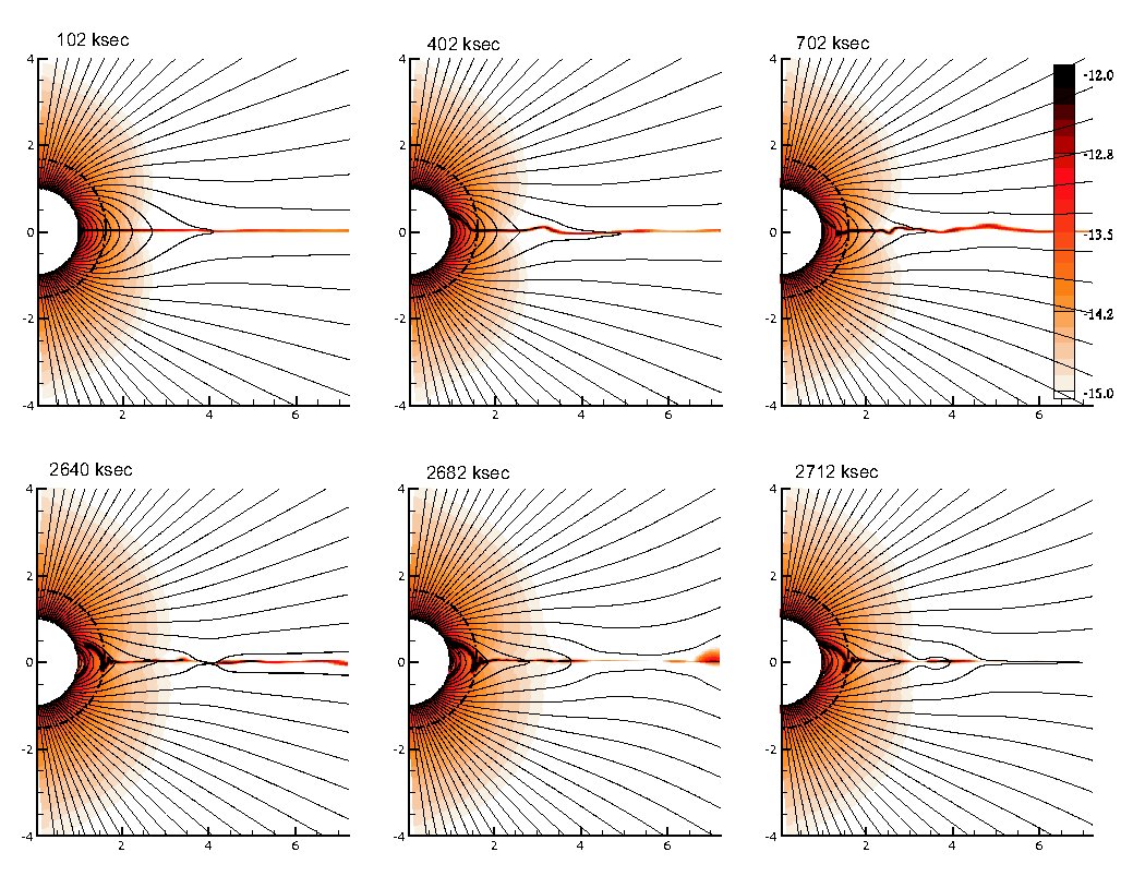
Figure 2: Snapshots of density (in cgs units on a logarithmic color-scale) and field lines (solid lines) at the labeled time intervals for the model with $\eta_{\ast}=100$ and $W=1/2$. The top panels show the model during a relatively quiescent period, when a dense rigidly rotating disk is being gradually built up. Note, however that material below the Kepler co-rotation radius ($R_{K}$, shown as a dashed circle) falls back onto the stellar surface, due to the lack of sufficient centrifugal support. The extent of the disk in this phase is determined by the magnetic field strength and extends up to the Alfvén radius $R_{\rm{A}}\approx 3.4R_{\ast}$, which is somewhat above the maximum outer radius of closed magnetic loops, $R_{\rm{c}}$. The bottom panels show the model later in the evolution, during one of the episodic centrifugal breakout events.

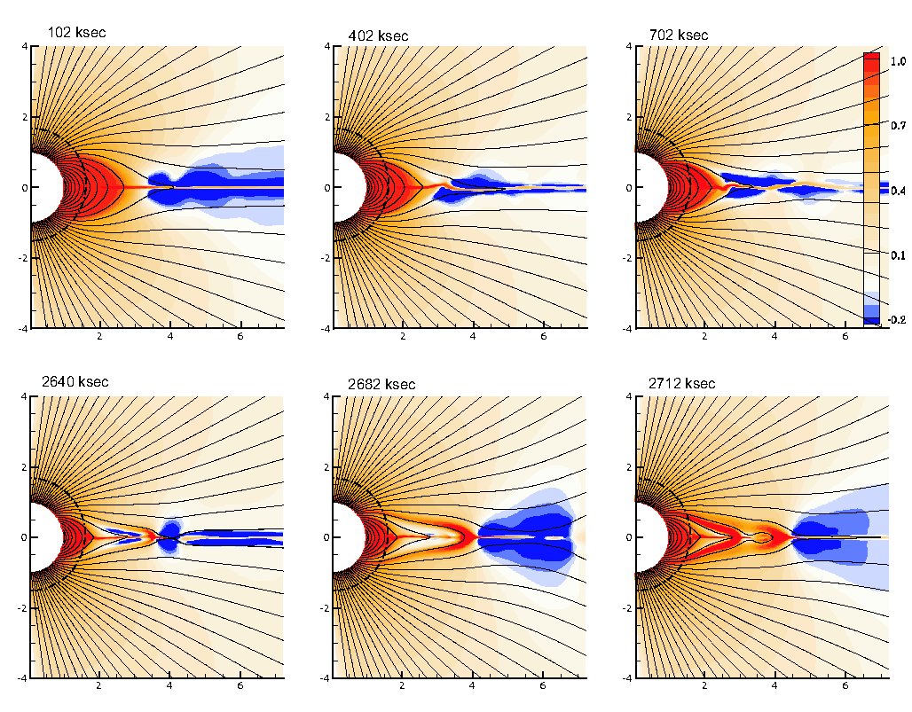
Figure 3: For the same model and same time snapshots as in figure 2, the azimuthal speed scaled by the local co-rotation speed, $\chi\equiv v_{\phi}/\Omega r\sin{\theta}$) . During the quiescent period the magnetosphere extends nearly to the closure radius $R_{\rm{c}}\approx 2.7R_{\ast}$, and co-rotates almost rigidly with the star (top panels). However, during episodic centrifugal breakouts (bottom panels) this rigidly rotating magnetosphere shrinks nearly to $R_{K}\approx 1.6R_{\ast}$, represented by the dashed circle. In addition to the mass lost to the breakout, this also helps some of the disk mass to leak inward as infall back onto the star.

4 RESULTS

4.1 Co-rotation and rigid disk

As a standard example to frame the overall study here, let us first focus on this case with confinement $\eta_{\ast}=100$ and rotation $W=1/2$ ($V_{\rm{rot}}=250$ km/s). Figures 2 show a series of time snapshots of the 2D spatial configuration of the magnetic field (solid lines), with the color scale representing logarithm of density; figure 3 give a similar time sequence for the azimuthal flow speed, scaled relative to the value that would occur in rigid-rotation, i.e. $\chi\equiv v_{\phi}(r)/\Omega r\sin\theta$, where $\Omega\equiv V_{\rm{rot}}/R_{\ast}$ is the star’s angular rotation frequency. The time snapshots were chosen to illustrate both relatively quiescent intervals (top panels), and phases with dynamic centrifugal breakout (bottom panels). The dashed circle represents the Kepler co-rotation radius at the equator ($R_{K}\approx 1.6R_{\ast}$).

In the evolution immediately following the initial condition, the magnetic field channels wind material toward the tops of closed loops near the equator, where the collision with the opposite stream leads to a dense disk-like structure (see top panels). But the gas is also generally torqued by the field, with, as can be seen in the upper panels of figure 3, material in the closed magnetosphere up to $R_{\rm{c}}\approx 2.7R_{\ast}$ kept nearly in rigid-body co-rotation with the star. Note that these closed, rigidly rotating loops thus extend through and beyond the Kepler radius. For any material trapped on loops below $R_{\rm{K}}$, the outward centrifugal support is less than the inward pull of gravity; since much of this material is compressed into clumps that are too dense to be significantly line-driven, it thus eventually falls back to the star following complex patterns along the closed-field loops.

By contrast, the dense material above the dashed line at $R_{\rm{K}}$ has a net radially outward force from the centrifugal acceleration vs. gravity. Still, during the initial build-up of this material at the tops of loops above $R_{\rm{K}}$, the magnetic field provides tension that is strong enough to hold it down, forming then a segment of the rigidly rotating disk predicted in the analytic RRM analysis by TO-05. However, much as anticipated in the Appendix of their paper, eventually material in the outer region of this RRM accumulates to sufficient density to force open the magnetic field, leading to the kind of centrifugally driven breakout events simulated in (ud-Doula et al., 2006). This is illustrated here in the bottom panels of figure 2.

Note however from figure 3 that certain regions, marked in blue, actually have a net azimuthal motion that is against the sense of the stellar rotation. This surprising and counterintuitive result is not a numerical artifact, but rather is related to a reverse torque effect that occurs in regions of rapid wind acceleration. This was first discussed by MacGregor & Friend (1987), who extended the classic Weber & Davis (1967) 1-D magnetic monopole rotation model for the solar wind to the case of the more rapidly accelerating line-driven winds. The 2-D analog for the dipole field here has little impact on our study of rotation and magnetic confinement, and so we defer further discussion to an upcoming paper that focuses on the role of the magnetic field in outward angular momentum transport and stellar spindown.

The centrifugal breakouts occuring in these simulations necessarily imply a breakdown in the basic formulation for ideal MHD within the Zeus code. In equatorial regions where the wind or centrifugal terms stretches out field lines of opposite polarity, the finite grid resolution allows effective reconnection, with the associated release of magnetic energy effectively lost instantaneously (e.g. due to radiative cooling) in these isothermal simulations. This is admittedly a simplified representation of the very complex physics thought to occur in actual reconnection, which indeed is an intense area of modern plasma physics research (, Shay et al.1999). But in the present context of driven reconnection, the overall global evolution seems likely to be set by the central competition between magnetic confinement and centrifugal breakout, with relatively little sensitivity to the details of local reconnection sites.

4.2 Global evolution of equatorial disk in radius and time

A key result of the simulations here is that there is really no true steady state possible, since the secular buildup of material in the disk must eventually lead to an episodic material breakout once the centrifugal forces overwhelm the finite magnetic tension. One primary goal of the more extensive parameter study here is to examine in detail the nature of this build-up and dissipation of mass in an RRM disk, and how this varies with the changes in the rotation rate and magnetic confinement. To facilitate illustration of these competing processes, let us define a radial mass distribution of the disk, computed at each radius $r$ in terms of the mass within some specified co-latitude range about the equator,

$$\frac{dm_{\rm{e}}(r,t)}{dr}\equiv 2\pi r^{2}\int_{\pi/2-\Delta\theta/2}^{\pi/2+\Delta\theta/2}\,\rho(r,\theta,t)\,\sin\theta\,d\theta\,.$$ (18)

To isolate the disk but not miss too much disk material during various oscillations about the equator, we choose a narrow, but not-too-limited range $\Delta\theta=10^{o}$. Figure 4 shows schematically how this is computed.

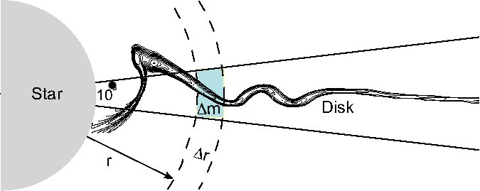
Figure 4: Schematic diagram illustrating the computation of the radial mass distribution of the equatorial disk, $dm_{e}/dr$ (see eqn. 18). We choose a cone angle of $\Delta\theta=10^{o}$ centered on the magnetic equator to encompass most of the material in the disk. We then compute the total mass $\Delta m$ contained in a narrow strip $\Delta r$ within the cone. Note, however, that some of the material may not lie within the cone during infall episodes.

For the same standard case ($W=0.5$, $\eta_{\ast}=100$) shown in figures 2 and 3, figure 5 shows a colorscale plot of this disk mass vs. radius (on the ordinate) and time (on the abscissa). The horizontal lines mark, from top to bottom, the estimated Alfvén radius $R_{\rm{A}}\approx 3.4R_{\ast}$, the loop closure radius $R_{\rm{c}}$, Kepler radius $R_{\rm{K}}\approx 1.6R_{\ast}$, and inner disk radius, $R_{in}\equiv(2/3)^{1/3}R_{\rm{K}}\approx 1.4R_{\ast}$ [see eqn. (19) of TO-05]. Within the RRM model, the last represents the location where the effective potential along a rigid-field loop first develops a local minimum, which can then trap material fed from the wind.

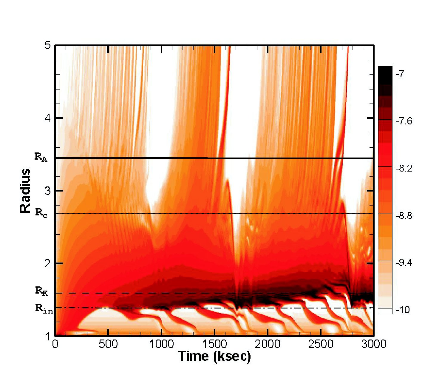
Figure 5: For MHD simulations of the standard model case with $\eta_{\ast}=100$ and $W=1/2$, the logarithm of the radial distribution of mass, $dm_{e}/dr$, within a cone of width $\Delta\theta=10^{o}$ centered on the equator, plotted vs. time and radius (in units of stellar radius). The color bar shows $\log(dm_{e}/dr)$ in units of $M_{\odot}/R_{\ast}$. The horizontal lines indicate the Alfvén radius $R_{\rm{A}}$ (solid), the maximum loop closure radius $R_{\rm{c}}$ (dotted), the Kepler radius $R_{\rm{K}}$ (dashed), and the inner RRM disk radius $R_{in}=(2/3)^{1/3}R_{\rm{K}}$ (dot-dashed). Note the accumulation of mass in a disk near the Kepler radius, and how this is limited both by relatively frequent (ca. every 200 ksec) intervals of downward infall, and by less-frequent (ca. every 1 Msec) major disruptions with substantial upward breakout.

The plot shows quite succinctly, and vividly, the global time evolution of the equatorial disk material. Initially mass builds up in the region around $R_{\rm{K}}$, but then there appear repeated episodes of infall of inner disk material back onto the star, about every 200 ksec or so. This leads to a gradual outward progression to the lower edge of the disk material.

But over a somewhat longer timescale, about every 1 Msec or so, there appears another, somewhat different kind of disruption, one that starts higher up, closer to the closure and Alfvén radii. This is characterized by outward ejection of the upper disk mass, but then also a “rebound” that propagates back down toward the Kepler radius, pushing the trapped disk material inward, and inducing a further leakage of disk mass through downward infall. The overall effect is to regulate the disk mass so that, by the end of the simulation at $t=3$ Msec, the addition of new material from the wind becomes roughly balanced by the losses to both infall and ejection.

The overall structure is certainly quite dynamic, but near the Kepler radius there nonetheless appears to be a quasi-permanent disk segment that corresponds roughly to what is predicted by the RRM analytic analysis of TO-05, as well as by the recent time-dependent Rigid-Field Hydrodynamics (RFHD) simulations of Townsend, Owocki, and ud-Doula (2007).

4.3 Comparison with RRM breakout analysis

Both the RRM and RFHD approaches are based on the idealization that the field is arbitrarily strong, and so remains perfectly rigid regardless of the amount of material in either the wind outflow or the disk buildup. But the associated discussion for both approaches recognized that the secular accumulation of material in the rigid-body disk would eventually cause the outward centrifugal forces to overwhelm the available inward tension associated with any large but finite magnetic field. In fact, the Appendix of TO-05 presents a simplified, but quantitative analysis of the resulting expected “breakout” of accumulated disk material. This anticipates, at least in general terms, several aspects of the processes seen in the present MHD simulations. In particular, it makes quite specific predictions for both the breakout timescales as a function of radius, and for the asymptotic mass accumulation near the Kepler radius. In this section, let us thus attempt a specific, semi-quantitative comparison between those predictions and the results of the MHD simulations.

4.3.1 Breakout timescale

Without benefit of the global dynamical picture available from the MHD simulations here, the TO-05 breakout analysis focused instead on the conditions for breakout at each local radius, conveniently scaled in terms of the Kepler radius as $\xi\equiv r/R_{\rm{K}}$. From TO-05 eqn. (A6) we find that, in terms of the free-fall time $t_{\rm{ff}}\equiv R_{\ast}/V_{\rm{esc}}$, the breakout time for some scaled outer disk radius $\xi_{\rm{o}}$ is given by

$$t_{\rm{b}}\approx\eta_{\ast}t_{\rm{ff}}\,\frac{6\xi_{\ast}/\xi_{\rm{o}}}{{\xi_{\rm{o}}}^{3}-1}\,.$$ (19)

Here we have approximated $\sqrt{\pi}/\mu_{\ast}\approx 2$ (cf. eqn. A8 of TO-05), and used the ratio of wind terminal speed to escape speed, $V_{\infty}/V_{\rm{esc}}\approx 3$, to convert the disk confinement parameter (also denoted $\eta_{\ast}$) in TO-05 into the wind confinement parameter defined here. Note also that the Kepler-scaled stellar radius can be written as $\xi_{\ast}=R_{\ast}/R_{\rm{K}}=W^{2/3}$.

Applying our stellar free-fall time $t_{\rm{ff}}\approx 19$ ksec, then for our standard ($\eta_{\ast}=100$, $W=1/2$) model, the predicted breakout time is

$$t_{\rm{b}}\approx\frac{7{\rm Msec}}{\xi_{\rm{o}}({\xi_{\rm{o}}}^{3}-1)}\,.$$ (20)

In the MHD simulations for this standard case, the breakouts seem to originate around $R_{\rm{c}}\approx 2.7R_{\ast}$, for example as indicated in figure 5 by the “bi-furcations” between upward and downward tracks that start at $r\mathrel{\hbox to0.0pt{\lower 3.0pt\hbox{$\mathchar 536\relax$}\hss}\raise 2.0pt\hbox{$\mathchar 316\relax$}}3R_{\ast}$ for times around 800, 1600, and 2700 ksec. If we thus approximate the outer disk radius by this maximum loop closure radius, we find $\xi_{\rm{o}}=R_{\rm{c}}/R_{\rm{K}}\approx 1.7$ and so $t_{\rm{b}}\approx 1$ Msec, about the timescale between major breakout eruptions seen in these same MHD simulations.

The TO-05 breakout analysis envisioned a hierarchy of breakout timescales, with more frequent eruptions occurring at larger radii; but its concluding paragraph also anticipated (partly based on early versions of the MHD simulations described here) that breakouts originating within $r\mathrel{\hbox to0.0pt{\lower 3.0pt\hbox{$\mathchar 536\relax$}\hss}\raise 2.0pt\hbox{$\mathchar 316\relax$}}2R_{\rm{K}}$ could also lead to substantial disruption of the entire magnetosphere. The simulations here do indeed show such major disruptions, but even after these there remains substantial mass near the Kepler radius.

Figure 6: Cumulative mass vs. time in MHD simulations for the standard model case. The top curve shows the total mass in the entire grid, i.e. including both disk and wind material. The middle curve shows the disk mass within $5^{o}$ of the equator, and within radii bounded by the inner RRM disk radius $R_{in}$ and an outer radius $R_{\rm{o}}=R_{\rm{c}}$. The bottom curve shows equatorial mass above this outer radius. The horizontal dashed line indicates the cumulative disk mass predicted by the RRM breakout analysis, using this same outer radius. Note that it matches quite well the varying asymptotic value of the middle curve, showing the disk mass in the MHD simulation.

4.3.2 Accumulated disk mass

For a disk with a scaled outer breakout radius $\xi_{\rm{o}}$, eqn. (A10) of TO-05 predicts a specific scaling for the total asymptotic disk mass, which in terms of the parameters here can be written,

$$m_{\rm{d}}(\xi_{\rm{o}}) = \frac{3\sqrt{\pi}\,{\dot{M}}\,t_{\rm{ff}}\,\eta_{\ast}\,W^{4/3}}{{\xi_{\rm{o}}}^{2}({\xi_{\rm{o}}}^{2}+\xi_{\rm{o}}+1)}$$ (21)

$$= 2.1\times 10^{-9}M_{\odot}\,\frac{\eta_{\ast}W^{4/3}}{{\xi_{\rm{o}}}^{2}({\xi_{\rm{o}}}^{2}+\xi_{\rm{o}}+1)}\,,$$

where the latter gives the numerical scaling for the stellar and wind parameters used here. If we then apply the confinement and parameters of our standard model, and use the characteristic breakout radius $\xi_{\rm{o}}\approx 1.7$ adopted above, we obtain a predicted total disk mass of $m_{\rm{d}}\approx 1.6\times 10^{-8}M_{\odot}$.

Figure 6 compares this predicted mass (red horizontal dashed curve) with the time variation of three types of cumulative mass in the standard model MHD results. Specifically, the top curve (black) shows the total integrated mass in the entire grid, including regions of both wind and disk; the middle curve (red) gives the cumulative mass in the equatorial disk region between the inner radius $R_{in}\approx 0.87R_{\rm{K}}\approx 1.4R_{\ast}$ and outer radius $R_{\rm{o}}\approx R_{\rm{c}}\approx 2.7R_{\ast}$; and finally, the bottom curve (blue) shows the equatorial mass above this outer disk radius, $r>R_{\rm{o}}\approx R_{\rm{c}}$.

Note in particular that the predicted asymptotic disk mass agrees remarkably well with this MHD simulation disk mass as shown by the middle, red curve. Of course, this is partly fortuitous, since just a 10% change in the choice of outer disk radius $\xi_{\rm{o}}$ would imply a ca. 40% change in disk mass. But the overall, order-magnitude agreement seems likely to be quite robust, and so provides a nice consistency check for both the RRM analysis and numerical simulations.

Comparison of the middle and upper curves in figure 6 further shows that the total mass in the thin, radially limited disk represents about half of the total mass in the entire model. In part, this reflects the fact that, for such a strong confinement model, a large fraction of the outgoing wind gets channeled into the disk. But another factor is that the wind material is flowing outward at a very high speed, and so has a much shorter “residency time” than the trapped, relatively static material in the disk.

4.3.3 Limitations of a localized breakout description

Despite this general success of the local breakout analysis in matching both the overall breakout timescale and the accumulated disk mass of this MHD simulation, the specifics of the dynamical evolution seen in the simulation make clear that the breakout process is really a global phenomenon. As the accumulation of material in the outer disk regions stresses and eventually overcomes the inward restraint of the magnetic field, the associated outward stretching alters the global field, including in the inner regions near the Kepler radius. Moreover, once a breakout occurs, the release of this stretching causes the inner, closed field lines to snap back inward, much like a stretched rubber band after release. The overshoot can push disk material below the Kepler radius and trigger infall back onto the star.

Overall, the wind-fed accumulation of disk mass is thus balanced not just by ejection outward, but also by infall inward. In contrast to the idealized picture of the breakout analysis, which formally predicts the timescale for breakout (and thus emptying) of material right at the Kepler radius to become arbitrarily long, the dynamic oscillation and associated inward spillage of material limits the asymptotic mass accumulated in this region. This new perspective on the dynamical nature of the disk mass budget has potentially important implications for modelling and interpreting observational diagnostics ( see Townsend et al. 2005; Townsend, Owocki & ud-Doula 2007).

4.4 Comparison with non-rotating model

To demonstrate further the role of rotation in how magnetic fields influence a wind outflow, let us now compare the results of this $\eta_{\ast}=100$, $W=1/2$ case with the corresponding non-rotating model. Figure 7 illustrates the dynamic evolution of equatorial mass for this strong-confinement case without rotation. Comparison with figure 5 shows that there are still both breakout and infall episodes, but now with both originating from nearly the same location, at roughly the loop closure radius $R_{\rm{c}}$. This infall from throughout most of the closed field region reflects the lack of any centrifugal support against gravity, and as such, there is no longer any accumulation of material into a circumstellar disk. The breakouts remain, but instead of being driven by centrifugal forces, these are now the result of entrainment of the field with the outflowing wind. The timescales for both breakout and infall are comparable to the rotating case, but seem somewhat more irregular. Overall, without the buildup in the disk, there is significantly less mass in the magnetosphere than in the rotating case.

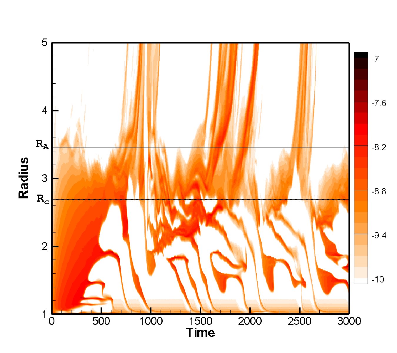
Figure 7: As in figure 5, the logarithm of the radial distribution of equatorial mass, $dm_{e}/dr$, again plotted vs. time and radius for a strong confinement ($\eta_{\ast}=100$) model, but now with no rotation ($W=0$). The horizontal lines indicate the Alfvén radius $R_{\rm{A}}$ (solid) and loop closure radius $R_{\rm{c}}$ (dotted). Note there are again complex patterns of breakout and infall, but now with more irregular timescales, and with the infall extending up to regions of breakout, near the loop closure radius. As such, there is no longer an extended region of mass accumulation into a circumstellar disk.

Figure 8: Top panel: Average mass loss rate (in units of the non-rotating, non-magnetic case) for MHD models with various rotational rates $W=0,1/4,1/2$ plotted against $\sqrt{\eta_{\ast}}\propto B_{\ast}$. Note that for $W=1/2$ the mass loss rate is nearly constant for models with high confinement $\eta_{\ast}>25$. Bottom panel: Corresponding mass loss rates from the analytic scaling formula in eqn. (24).

4.5 Results for variation in parameters

To provide a wider context to these detailed results for specific cases with strong confinement, let us now analyze results spanning a broader range of the 2-D parameter space for rotation and confinement strength. Before focusing further on equatorial disk material, let us first briefly consider the effects of various magnetic field strengths and rotation rates on the global mass loss from the stellar wind.

4.5.1 Global mass loss

As discussed in Paper I, one general effect of a strong magnetic field on a wind is the confinement and inhibition of the outflow within a belt around the magnetic equator. For a dipole field line that reaches up to the maximum closure radius $R_{\rm{c}}$, the co-latitude $\theta_{c}$ at the surface footpoint satisfies

$$\sin\theta_{\rm{c}}=\sqrt{R_{\ast}/R_{\rm{c}}}\,,$$ (22)

The fraction of the stellar surface area that is covered by closed field lines is given by $\cos\theta_{\rm{c}}$, leaving thus only the remaining fraction $1-\cos\theta_{\rm{c}}$ as the source of wind mass loss. For the non-rotating case, we can thus use this open-field fraction to estimate the overall magnetic reduction in the mass loss rate,

$$\frac{{\dot{M}_{\rm{B}}}}{{\dot{M}_{\rm{B}=0}}}\approx 1-\sqrt{1-R_{\ast}/R_{\rm{c}}}\,,$$ (23)

where $R_{\rm{c}}$ is evaluated from eqn. (10), with the Alfvén radius $R_{\rm{A}}$ from eqn. (9) using $q=3$. Note that this ignores higher order effects, such as the reduction of the mass flux in open field regions due to the tilt of surface field relative to the radial direction for wind driving (see Owocki & ud-Doula, 2004).

The two panels in figure 8 compare the mass loss rate vs. $\sqrt{\eta_{\ast}}$ ($\propto B$) for both simple analytic scalings (bottom) and results of numerical MHD simulations (top), with the lower, middle, and upper curves in each panel corresponding to the $W=0$, 1/4, and 1/2 rotation models. For the non-rotating case, the numerical and analytic results shown in the lower curves are in good overall agreement. But for the rotating case, the upper curves in the top panel show that the tendency of the strong field to reduce the overall mass loss rate is somewhat compensated by faster rotation, and in the $W=1/2$ case, even flattens to nearly constant toward the limit of strong confinement. This reflects the additional effect of centrifugal forces in driving the breakout of material initially trapped in closed loops near and below the confinement radius $R_{\rm{c}}$. In effect, the rotation allows eventual breakout from loops that are some factor times the Kepler radius, say $2R_{\rm{K}}$.

To take this into account in an analytic scaling formula, the upper two curves in the lower panel use a modified form of eqn. (23),

$$\frac{{\dot{M}_{\rm{B}}}}{{\dot{M}_{\rm{B}=0}}}\approx 1-\sqrt{1-R_{\ast}/R_{\rm{c}}}+1-\sqrt{1-0.5*R_{\ast}/R_{\rm{K}}}\,,$$ (24)

which effectively sums separate contributions from polar opening and rotational breakout, with the closure and Kepler radii computed from eqns. (9), (10), and (14). With this generalized scaling, the overall variations of the analytic curves in the lower panel roughly match the corresponding MHD results in the upper panel.

Figure 9: Logarithm of radial distribution of equatorial disk mass, $dm_{e}/dr$ vs. radius and time, for a mosaic of models with magnetic confinements $\log(\eta_{\ast})=$ 1/2, 1, 3/2, 2, 5/2 and 3 (columns from left) and rotations $W=$ 0, 1/4, and 1/2 (rows from bottom) with the same contour levels and the ranges for time and radius as in figure 5. Again, the horizontal lines indicate the Alfvén radius $R_{\rm{A}}$ (solid) and the Kepler radius $R_{\rm{K}}$ (dashed).

4.5.2 Equatorial mass and disk

Let us next examine how the equatorial disk region is affected by variations in the magnetic confinement and rotation parameters. Figure 9 compares the radius and time evolution of the equatorial mass, $dm_{e}/dr$, for an mosaic of models with various $\eta_{\ast}$ and $W$. The comparison provides a global overview of how the equatorial mass evolution is affected by changes in confinement and rotation.

For weak rotation and confinement cases in the lower left panels, material generally escapes outward without much infall, with only a modest rotational enhancement in mass loss. But most other models again show a complex competition between infall and breakout, with the latter always being less frequent and stronger.

In particular, this complex combination of infall and breakout also dominates the $R_{\rm{A}}\approx R_{\rm{K}}$ transition models identified in figure 1, i.e. the ones here with $\log\eta_{\ast}=1/2$ and $W=1/2$ or $\log\eta_{\ast}=3/2$ and $W=1/4$. Such models might seem optimally fine-tuned to propel material into Keplerian orbit, and yet they show no apparent tendency for material to accumulate into the extended, Keplerian disk envisioned in the MTD scenario suggested by Cassinelli et al. (2002). The lack of a sharp outer cutoff in the large-scale dipole field makes it incompatible with the shear of a Keplerian disk, and without the closed loops that hold down a rigid disk in the strong-confinement limit, material is propelled outward to escape, rather than into a stable Keplerian orbit.

As expected, accumulation into such a rigid-body disk is strongest for the fastest rotation, and strongest confinement, as shown by models at the upper right. For strong confinement but slow or no rotation, the material infall comes from a greater height, set by the closure radius, which increases roughly as $R_{\rm{c}}\sim\eta_{\ast}^{1/4}$.

This larger infall height seems also to lead to a somewhat longer infall timescale. Likewise, the breakout timescale also seems to increase for models with stronger confinement paramater $\eta_{\ast}$, but not quite in the linear proportion that might be suggested by eqn. (19). The reason is that the scaled outer confinement radius $\xi_{\rm{o}}$ appears in the denominator, and since this also increases with confinement through it dependence on the closure the radius $R_{\rm{c}}$, the net effect is to weaken the $\eta_{\ast}$ sensitivity of $t_{\rm{b}}$, especially in the strong confinement limit $\eta_{\ast}\gg 1$.

Note also that the $W=1/2$ rotation model with the strongest confinement, $\eta_{\ast}=1000$, is relatively stable, without the repeated equatorial infall events seen in other models. Instead of the extensive north-south disk oscillations seen in other models, in this case the variations of the equatorial disk are mostly symmetric about the equator, and thus do not induce as much “spillage” back onto the star. The recent analysis of “Rigid-Field Hydrodynamics” (RFHD) models by Townsend et al. (2007) show that both types of oscillation modes are allowed, with the one dominating in simulations depending on subtle details of the excitation processes.

But overall, it seems that the basic principals gleaned from the detailed study of the standard, strong-confinement case can be quite logically generalized to understand the trends in properties seen from this mosaic of models spanning a broad range of rotation and confinement parameters.

5 SUMMARY & FUTURE WORK

This paper examines the effects of field-aligned rotation on the magnetic channeling and confinement of a radiatively driven stellar wind. It builds upon the non-rotating models of Paper I, extending them to cases of much stronger magnetic confinement (up to $\eta_{\ast}=1000$), and comparing a full spectrum of models ranging from weak to strong confinement at equatorial rotation rates from zero to a substantial fraction ($W=$ 1/4 and 1/2) of the critical (or orbital) limit. As an initial study, it ignores the effects of oblateness, gravity darkening and limb darkening, and is based on an idealization of isothermal flow driven by a purely radial line-force.

The key results can be summarized as follows:

• The 2-D parameter space represented by rotation $W$ and magnetic confinement $\eta_{\ast}$ can be conveniently divided by comparing the Kepler radius $R_{\rm{K}}\approx W^{-2/3}R_{\ast}$ with the Alfvén radius $R_{\rm{A}}\approx\eta^{1/4}R_{\ast}$.

• Models with $R_{\rm{A}}<R_{\rm{K}}$ have weak rotation and/or magnetic confinement, with the effects of rotation limited to some modest enhancement in equatorial density and overall mass loss rate, relative to non-rotating cases. In general any magnetically confined material falls back to the star.

• Transition models with $R_{\rm{A}}\approx R_{\rm{K}}$ have a complex combination of inner region infall and outer region breakout, but show no signs of accumulation of material into the kind of extended Keplerian disk posited in the magnetically torqued disk paradigm of Cassinelli et al. (2002).

• In models with $R_{\rm{A}}>R_{\rm{K}}$ the strong magnetic confinement combines with a sufficiently rapid rotation that can support material against infall near and above the Kepler radius, with then the magnetic field both holding material in nearly rigid-body rotation, and keeping it confined against the tendency for the centrifugal force to propel material outward against gravity.

• Such strongly confined rotation models show a clear accumulation into a rigid-body disk, much as predicted in the analytic Rigidly Rotating Magnetosphere (RRM) formalism of TO-05.

• However, the present MHD simulations show that such rigid-body disks can be highly dynamic and variable, with mass accumulation regulated by a complex combination of inner disk infall and outer disk breakout.

• Nonetheless, application of the simple breakout analysis introduced by TO-05 – slightly modified to identify the outer disk limit with the maximum radius of loop closure – provides a quite good, semi-quantitive agreement with both the breakout timescale and limiting disk mass of the MHD simulations.

• The breakout events here are similar to those discussed by ud-Doula, Townsend, and Owocki (2006), except the assumption here of isothermal flow precludes us from following that paper’s specific application to modelling X-ray flares.

There thus remains much work for future extensions of the present study, including relaxation of the assumptions of isothermal flow, purely radial driving, 2-D axisymmetry with aligned dipole field, and moderate rotation rates for which stellar oblateness can be neglected.

To more fully test the RRM paradigm, there is also a need to extend MHD simulations even further into the large confinement limit, to approach as closely as possible the estimated $\eta_{\ast}\approx 10^{7}$ appropriate for Bp stars like $\sigma$ Ori E.

But even within the context the present set of models, we have ignored here another key effect of magnetic rotation, namely the outward angular momentum loss in the stellar wind, and the associated spindown of the underlying star. This omission was made to allow a more directed focus on the already quite interesting, complex, and subtle effects of rotation on magnetic confinement and disk formation. But we have already carried out an extensive analysis of the implications of our study for angular momentum loss and stellar spindown, and so intend this to be the subject for the next paper in this series.

Appendix A Maximum Polar Alfvén Speed

We derive here eqn. (17) cited in section 3.3, giving a simple scaling relation between the expected maximum polar Alfvén speed and the wind magnetic confinement parameter. We begin by repeating eqn. (7) relating the ratio of magentic to wind energy density to the ratio of Alfvén speed to flow speed,

$$\eta(r)\equiv\frac{B^{2}/8\pi}{\rho v^{2}/2}=\left(\frac{V_{\rm{A}}}{v}\right)^{2}\,.$$ (25)

Here the density $\rho$ can be eliminated by noting that, for a steady-state, magnetically channeled flow, the lack of divergence in both the field and mass flux requires,

$$\frac{4\pi\rho v}{B}=~{}{\rm constant}\equiv\frac{{\dot{M}}}{B_{\rm{p}}R_{\ast}^{2}}\,,$$ (26)

where we have normalized in terms of a polar surface field $B_{\rm{p}}$ and global mass flux ${\dot{M}}$. For a polar field that declines with radius as $B=B_{p}(R_{\ast}/r)^{q}$, this gives for the polar Alfvén speed,

$$V_{\rm{Ap}}^{2}=\frac{B_{\rm{p}}R_{\ast}^{2}}{{\dot{M}}}Bv=4\eta_{\ast}\,\left(\frac{R_{\ast}}{r}\right)^{q}vV_{\infty}\,,$$ (27)

where the latter equality casts this in term of the magnetic confinement parameter, with the factor 4 correcting for the fact that our standard $\eta_{\ast}$ is defined in terms of the equatorial surface field $B_{eq}$, which is half the polar value $B_{p}$. If we further assume a standard $\beta=1$ velocity law, then

$$V_{\rm{Ap}}=2\sqrt{\eta_{\ast}}\,V_{\infty}\left(1-\frac{R_{\ast}}{r}\right)^{1/2}\,\left(\frac{R_{\ast}}{r}\right)^{q/2}\,.$$ (28)

Setting the radial derivative of this to zero shows that the maximum occurs at radius $r=(1+1/q)R_{\ast}$, i.e. at $r=(4/3)R_{\ast}$ for the standard dipole case with $q=3$. Plugging this radius into eqn. (28), we find that the expected maximum Alfvén speed for dipole expansion of the polar wind is

$$\max(V_{Ap})=\frac{\sqrt{27}}{8}\,\sqrt{\eta_{\ast}}\,V_{\infty}\approx 0.65\,\sqrt{\eta_{\ast}}\,V_{\infty}\,.$$ (29)

This thus provides a simple rule for the maximum Alfvén speed to allow in running MHD simulations with increasing magnetic confinement parameter, as discussed in section 3.3.

References

- Babel & Montmerle (1997a) Babel J., Montmerle T., 1997a, ApJ, 485, L29
- Babel & Montmerle (1997b) Babel J., Montmerle T., 1997b, A&A, 323, 121
- Cassinelli et al. (2002) Cassinelli J. P., Brown J. C., Maheswaran M., Miller N. A., Telfer D. C., 2002, ApJ, 578, 951
- Castor et al. (1975) Castor J. I., Abbott D. C., Klein R. I., 1975, ApJ, 195, 157
- Conti & Ebbets (1977) Conti P. S., Ebbets D., 1977, ApJ, 213, 438
- Donati et al. (2002) Donati J.-F., Babel J., Harries T. J., Howarth I. D., Petit P., Semel M., 2002, MNRAS, 333, 55
- Donati et al. (2006) Donati J.-F., Howarth I. D., Jardine M. M., Petit P., Catala C., Landstreet J. D., Bouret J.-C., Alecian E., Barnes J. R., Forveille T., Paletou F., Manset N., 2006, MNRAS, 370, 629
- Drew (1989) Drew J. E., 1989, ApJS, 71, 267
- Falle (2002) Falle, S. A. E. G. 2002, ApJ, 577, L123
- Friend & Abbott (1986) Friend D. B., Abbott D. C., 1986, ApJ, 311, 701
- Fukuda (1982) Fukuda I., 1982, PASP, 94, 271
- Gagné et al. (2005) Gagné M., Oksala M. E., Cohen D. H., Tonnesen S. K., ud-Doula A., Owocki S. P., Townsend R. H. D., MacFarlane J. J., 2005, ApJ, 628, 986
- Gayley & Owocki (2000) Gayley K. G., Owocki S. P., 2000, ApJ, 537, 461
- MacGregor & Friend (1987) MacGregor K. B., Friend D. B., 1987, ApJ, 312, 659
- Owocki (2006) Owocki S., 2006, in Kraus M., Miroshnichenko A. S., eds, Stars with the B[e] Phenomenon Vol. 355 of Astronomical Society of the Pacific Conference Series, Formation and Evolution of Disks around Classical Be Stars. pp 219–+
- Owocki et al. (2006a) Owocki S., Townsend R., ud-Doula A., 2006a, in 36th COSPAR Scientific Assembly Vol. 36 of COSPAR, Plenary Meeting, Magnetic Coupling between Hot Stars and their Radiatively Driven Winds and Decretion Disks. pp 3548–+
- Owocki et al. (2006b) Owocki S., Townsend R., ud-Doula A., 2006b, Physics of Plasmas
- Owocki & ud-Doula (2003) Owocki S., ud-Doula A., 2003, in Balona L. A., Henrichs H. F., Medupe R., eds, Astronomical Society of the Pacific Conference Series Vol. 305 of Astronomical Society of the Pacific Conference Series, Magnetic Spin-Up of Line-Driven Stellar Winds. pp 350–+
- Owocki et al. (1996) Owocki S. P., Cranmer S. R., Gayley K. G., 1996, ApJ, 472, L115+
- Owocki & ud-Doula (2004) Owocki S. P., ud-Doula A., 2004, ApJ, 600, 1004
- Pauldrach (1987) Pauldrach A., 1987, A&A, 183, 295
- Pauldrach et al. (1985) Pauldrach A., Puls J., Hummer D. G., Kudritzki R. P., 1985, A&A, 148, L1
- (23) Shay, M. A., Drake, J. F., Rogers, B. N., & Denton, R. E. 1999, Geophys. Res. Lett., 26, 2163
- Stone & Norman (1992) Stone J. M., Norman M. L., 1992, ApJS, 80, 753
- Townsend & Owocki (2005) Townsend R. H. D., Owocki S. P., 2005, MNRAS, 357, 251
- Townsend et al. (2005) Townsend R. H. D., Owocki S. P., Groote D., 2005, ApJ, 630, L81
- Townsend et al. (2007) Townsend R. H. D., Owocki S. P., ud-Doula A., 2007, MNRAS, in press, 709
- ud-Doula (2003) ud-Doula A., 2003, PhD thesis, University of Delaware
- ud-Doula & Owocki (2002) ud-Doula A., Owocki S. P., 2002, ApJ, 576, 413
- ud-Doula et al. (2006) ud-Doula A., Townsend R. H. D., Owocki S. P., 2006, ApJ, 640, L191
- Walborn (1981) Walborn N. R., 1981, ApJ, 243, L37
- Weber & Davis (1967) Weber E. J., Davis L. J., 1967, ApJ, 148, 217