High-resolution radio observations of submillimetre galaxies

Abstract

We have produced sensitive, high-resolution radio maps of 12 submillimetre (submm) galaxies (SMGs) in the Lockman Hole using combined Multi-Element Radio-Linked Interferometer Network (MERLIN) and Very Large Array (VLA) data at a frequency of 1.4 GHz. Integrating for 350 hr yielded an r.m.s. noise of 6.0 $\mu$Jy beam^-1 and a resolution of 0.2–0.5 arcsec. For the first time, wide-field data from the two arrays have been combined in the ($u,v$) plane and the bandwidth smearing response of the VLA data has been removed. All of the SMGs are detected in our maps as well as sources comprising a non-submm luminous control sample. We find evidence that SMGs are more extended than the general $\mu$Jy radio population and that therefore, unlike in local ultraluminous infrared galaxies (ULIRGs), the starburst component of the radio emission is extended and not confined to the galactic nucleus. For the eight sources with redshifts we measure linear sizes between 1 and 8 kpc with a median of 5 kpc. Therefore, they are in general larger than local ULIRGs which may support an early-stage merger scenario for the starburst trigger. X-rays betray active galactic nuclei (AGN) in six of the 33 sources in the combined sample. All but one of these are in the control sample, suggesting a lower incidence of AGN amongst the submm-luminous galaxies which is, in turn, consistent with increased X-ray absorption in these dust-obscured starbursts. Only one of our sources is resolved into multiple, distinct components with our high-resolution data. Finally, compared to a previous study of faint radio sources in the GOODS-N field we find systematically smaller source sizes and no evidence for a tail extending to $\sim$4 arcsec. Possible reasons for this are discussed.

1 Introduction

Table 1: Lockman Hole SMGs included in our sample. Positions and 1.4-GHz flux densities are taken from the VLA catalogue of Biggs & Ivison (2006). Redshifts are determined spectroscopically and are taken from either Chapman et al. (2005) or Ivison et al. (2005, 2007).

ID	SHADES ID	MAMBO ID	Bolocam ID	Radio position (J2000)	$S_{1.4}$ ($\mu$Jy)	$z$
SMG01	LOCK850.01	LH 1200.005	1100.014	10:52:01.250 +57:24:45.76	73	2.148
SMG02	LOCK850.04	LH 1200.003		10:52:04.226 +57:26:55.46	66	1.48
SMG03	LOCK850.09	LH 1200.042		10:52:15.634 +57:25:04.27	58	1.853
SMG04	LOCK850.16	LH 1200.096		10:51:51.690 +57:26:36.09	110	1.147
SMG05	LOCK850.17	LH 1200.011		10:51:58.018 +57:18:00.26	93	2.239
SMG06	LOCK850.30			10:52:07.489 +57:19:04.01	246	2.689
SMG07	LOCK850.33	LH 1200.012		10:51:55.470 +57:23:12.75	54	2.686
SMG08	LOCK850.71			10:52:19.086 +57:18:57.87	98
SMG09	LOCK850.87			10:51:53.362 +57:17:30.06	93
SMG10		LH 1200.008		10:51:41.431 +57:19:51.90	295	1.212
SMG11			1100.003$a$	10:52:13.376 +57:16:05.41	249
SMG12			1100.003$b$	10:52:12.256 +57:15:49.59	85

SMGs form a class of object that was unknown before the advent of modern bolometer arrays – starting with the Submillimetre Common User Bolometer Array (SCUBA; Holland et al., 1999) – in the late 1990s (Smail, Ivison & Blain, 1997). Effective follow-up of these sources has been particularly difficult due to the large positional uncertainty of the submm detections. As a result, most of our understanding of the properties of these sources has been made possible by deep, wide-field radio imaging, which exploits the radio/far-infrared (far-IR) correlation to produce positions with sub-arcsecond accuracy (e.g. Ivison et al., 2002, 2007). It is now known that SMGs lie at high redshift (Chapman et al., 2003, 2005) and it is believed that their large far-IR luminosities are due to the ultraviolet (UV) light produced by intense star formation ($\geq$1000 M_☉ yr^-1) being reprocessed by dust; as such they are major contributors to the star-formation history of the Universe (Hughes et al., 1998).

Although the emission from SMGs is believed to originate predominantly from a starburst, there is likely to be a contribution from an AGN in some sources. Signatures of AGN include X-ray emission (Alexander et al., 2003, 2005), compact or jet/lobe radio emission (Chapman et al., 2004; Muxlow et al., 2005; Garrett et al., 2001), unusual radio spectral indices as well as certain line characteristics seen in optical (Swinbank et al., 2004) and mid-IR spectroscopy (Menéndez-Delmestre et al., 2007; Lutz et al., 2005). Star formation and AGN activity are believed to be closely linked due to the well-established correlation between black hole and bulge mass in nearby elliptical galaxies (Magorrian et al., 1998; Marconi & Hunt, 2003; Häring & Rix, 2004) and, furthermore, feedback mechanisms have been proposed whereby star formation is regulated by the AGN (e.g. Silk & Rees, 1998; Di Matteo, Springel & Hernquist, 2005). Page et al. (2004) have suggested an evolutionary sequence within which the transition from X-ray absorbed to unabsorbed AGN represents the termination of galaxy growth.

In order to investigate the origin of the radio emission in SMGs, we have obtained high-resolution imaging of the Lockman Hole with MERLIN, a grouping of seven telescopes across the United Kingdom. The maximum distance between telescopes, 215 km, corresponds to an angular resolution of $\sim$200 milliarcsec (mas) at a frequency of 1.4 GHz, much higher than that obtained with the VLA at the same frequency. The Lockman Hole is notable for its very low Galactic H i column density (Lockman, Jahoda & McCammon, 1986) and has been targeted by a number of different instruments at different wavelengths, including XMM-Newton (Hasinger et al., 2001; Mainieri et al., 2002; Brunner et al., 2007), Spitzer (Huang et al., 2004; Egami et al., 2004) and the VLA (De Ruiter et al., 1997; Ciliegi et al., 2000; Ivison et al., 2002).

In this paper we combine our new MERLIN data with existing VLA data in order to increase the sensitivity to extended emission that would otherwise be resolved out or poorly constrained due to the lack of short spacings, whilst still retaining significantly higher resolution than can be obtained with the VLA alone. The paper is structured as follows. In the next section we describe the sample of SMGs as well as a control sample with which the structures of the SMGs can be compared. In §3 we describe the observations and the data analysis, including a new technique for combining radio interferometric wide-field data in the Fourier plane, and present the maps. Discussion of our results and conclusions follow in §4 and 5.

2 Sample selection

2.1 SMGs

In the submm waveband, the Lockman Hole has been targeted in several overlapping surveys: at 850 $\mu$m (Scott et al., 2002; Coppin et al., 2006) with SCUBA on the James Clerk Maxwell Telescope (JCMT), at 1200 $\mu$m with the Max-Planck Millimeter Bolometer array (MAMBO) on the Institut de Radio Astronomie Millimétrique’s (IRAM’s) 30-m telescope (Greve et al., 2004) and at 350 and 1100 $\mu$m with SHARC ii (Laurent et al., 2006) and Bolocam (Laurent et al., 2005), respectively, at the Caltech Submillimeter Observatory (CSO). The Lockman Hole portion of the SCUBA Half-Degree Extragalactic Survey (SHADES; Mortier et al., 2005; Coppin et al., 2006) found the largest number of sources: 60 SMGs at 850 $\mu$m over an area of approximately 360 arcmin². This included data from the 8-mJy Survey (Scott et al., 2002; Fox et al., 2002). Combining source lists from several surveys has been used as a check on the robustness of individual sources (Ivison et al., 2005).

Our sample was compiled from the above references and comprises all SMGs within 6 arcmin of the MERLIN and VLA pointing centre ($\mathrm{10^{h}\,52^{m}\,08\aas@@fstack{s}82,+57^{\circ}\,21^{\prime}\,33\aas@@fstack{\prime\prime}8}$, J2000) that have a peak radio flux density (as measured with the VLA) in excess of 50 $\mu$Jy. The radial cutoff is required to ensure that the radio data are minimally effected by bandwidth and time smearing (§3.3) and primary beam effects. The primary beam for unequal apertures has been investigated by Strom (2004) and for baselines with the most disparate telescope sizes (76 m–25 m) is equal to 15.6 arcmin (fwhm), significantly in excess of our 12-arcmin diameter field.

With these constraints we obtain a sample of 12 SMGs which we list in Table 1, nine of which were detected by SHADES. A number of these sources are also detected by MAMBO and or Bolocam/SHARC ii. The three remaining sources were only detected by either MAMBO or Bolocam/SHARC ii; the radio identification (ID) is unambiguous in each case. For LH 1200.008 (Greve et al., 2004; Ivison et al., 2005), there is only a single, relatively bright radio source located near the submm position. The remaining SMG, 1100.003 (Laurent et al., 2005), was originally detected by Bolocam and shown by later observations with SHARC  ii (Laurent et al., 2006) to be a blend of two sources. Both of these have a radio counterpart; we refer to them as 1100.003a and 1100.003b respectively, where 1100.003a is much the brighter of the two in the radio. Flux densities and positions for all sources are taken from Biggs & Ivison (2006) and spectroscopic redshifts (available for seven of the SMGs) from Chapman et al. (2005) or Ivison et al. (2005, 2007).

2.2 Control sample

As well as the SMG sample, we have defined a control sample with which the properties of the SMGs can be contrasted. This sample is made up of the remaining VLA detections within the 6-arcmin radius area that have peak brightnesses greater than 50 $\mu$Jy beam^-1 i.e. it is defined in an identical fashion to the SMG sample. Of these, we exclude one obviously resolved source which is much brighter than the others, its total flux density exceeding 1 mJy. This gives a control sample of 21 sources.

Figure 1: VLA 1.4-GHz map of the Lockman Hole, showing the positions of the SMGs (circles) and the control sample (squares). Also marked is the 6-arcmin radial cutoff used in defining our samples and the centre of the field.

Table 2: Radio sources with peak flux densities greater than 50 $\mu$Jy beam^-1 which lie within 6 arcmin of the phase centre and which do not have submm detections. These constitute our control sample. Flux densities and positions are taken from the VLA catalogue of Biggs & Ivison (2006).

ID	Radio position (J2000)	$S_{1.4}$ ($\mu$Jy)
C01	10:51:25.892 +57:21:54.61	78
C02	10:51:39.588 +57:17:32.06	58
C03	10:51:44.431 +57:22:03.74	54
C04	10:51:44.492 +57:17:19.66	137
C05	10:51:49.939 +57:25:21.73	83
C06	10:51:50.113 +57:26:35.73	115
C07	10:51:58.150 +57:26:01.13	62
C08	10:51:58.919 +57:23:30.13	224
C09	10:52:05.491 +57:17:09.99	85
C10	10:52:12.493 +57:24:52.91	222
C11	10:52:13.283 +57:26:50.36	52
C12	10:52:16.903 +57:20:17.24	108
C13	10:52:17.615 +57:21:27.37	160
C14	10:52:29.740 +57:17:53.31	89
C15	10:52:31.522 +57:17:51.67	56
C16	10:52:31.849 +57:24:50.39	55
C17	10:52:32.877 +57:25:42.74	115
C18	10:52:33.748 +57:17:58.85	62
C19	10:52:37.370 +57:21:48.15	155
C20	10:52:39.600 +57:24:31.37	143
C21	10:52:42.418 +57:19:14.59	253

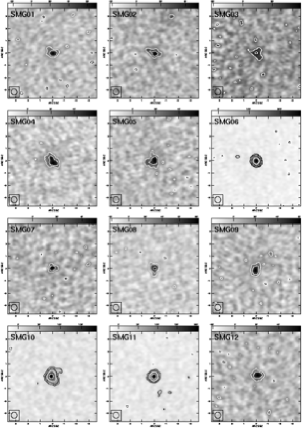
Figure 2: Stokes $I$ maps of the 12 SMGs in our Lockman Hole sample. The beam is shown in the bottom-left corner and has dimensions of $521\times 481$ mas² at a position angle of $23\aas@@fstack{\circ}6$. The greyscale has units of $\mu$Jy beam^-1 and contours are drawn at $-1$, 1, 2, 4, 8, etc. times the 3 $\sigma$ noise (3 $\times$ 6.0 $\mu$Jy beam^-1).

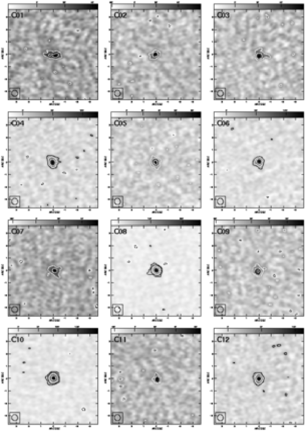
Figure 3: Stokes $I$ maps of the sources in the control sample. Contours, beamsizes and greyscales are the same as for Fig. 2.

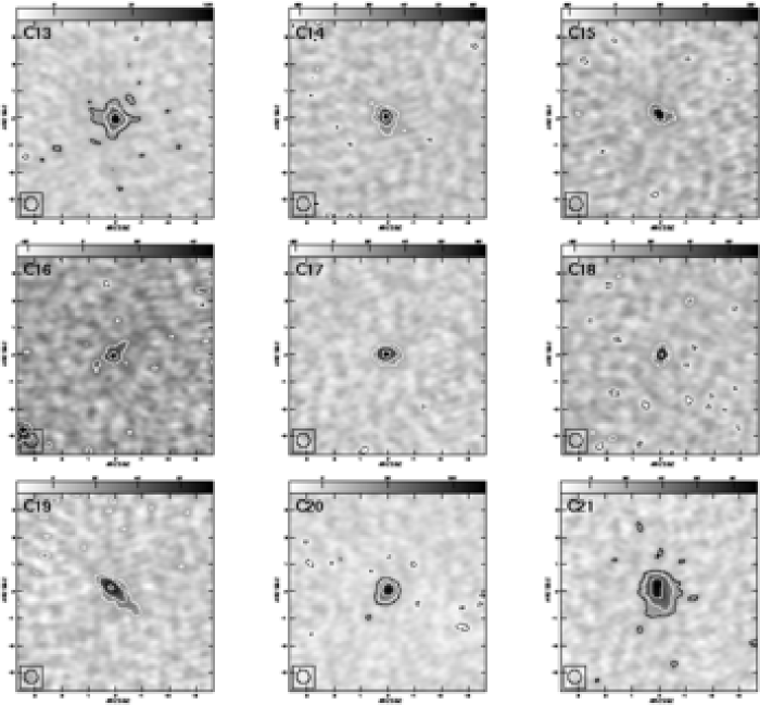
Figure 4: continued

3 Observations and data reduction

3.1 VLA

The VLA data were first discussed in Ivison et al. (2002) and we give only a brief summary here. The standard VLA wide-field ‘pseudo continuum’ mode was used, two separate frequency bands near 1400 MHz (both containing right and left circular polarisations, RCP and LCP) split into seven 3.125-MHz-wide channels each. The correlator integration time was 5 s. The full primary beam was mapped, with imagr, and the data self-calibrated using a model of the sky (including bright sources in the primary beam sidelobes). The data from the several days of observations were then combined with stuffr and produced final maps with an r.m.s. noise of approximately 5 $\mu$Jy beam^-1. In order to simplify later mapping of the combined MERLIN/VLA dataset, the VLA data had all clean components which lay further than 6 arcmin from the phase centre subtracted using uvsub. In this way, mapping with the very large combined dataset could be confined to the central regions of the primary beam, the sidelobe response from brighter, more distant sources already having been removed.

3.2 MERLIN

The MERLIN data were observed over the period 2005 March to June using all seven telescopes, including the 76-m Lovell telescope which approximately doubles the sensitivity. A single 16-MHz band with a central frequency of 1408 MHz was split by the correlator into 32 separate 0.5-MHz wide channels with data produced every 4 s. The receivers were sensitive to both RCP and LCP, but a lack of correlator capacity does not allow the cross-correlation of the RCP and LCP data necessary for polarisation imaging. Phase referencing was accomplished using the nearby source, J1058+5628, with approximately 6 min spent observing the target and 2 min on the calibrator. In total, the Lockman Hole was observed for $\sim$290 h; this corresponds to an expected image sensitivity of $\sim$6 $\mu$Jy beam^-1. Absolute flux calibration was based on observations of 3C 286 and bandpass calibration with either OQ 208 or DA 193.

Initial flux and bandpass calibration took place in the usual manner with subsequent processing undertaken using the National Radio Astronomy Observatory’s aips package. Gain solutions, first in phase and then in amplitude and phase were derived from the phase calibrator data and interpolated onto the target. The calibrated data were subsequently combined into a single dataset using stuffr. As with Muxlow et al. (2005), four of the outer channels were not included when mapping as these reduced the image sensitivity. At this stage it is usual to scale the data weights to reflect the nominal sensitivity of each telescope. In preference to this, we have used fixwt to set the weights based on the scatter in the data; this causes the weights to reflect the relative sensitivity of each telescope, additionally as a function of time (caused by, for example, the changing antenna elevation).

In preparation for combining these data with those from the VLA, maps were made of sources identified with the VLA using imagr with natural weighting. Those sources which were detected and were located further than 6 arcmin from the phase centre had their clean components subtracted from the data, as with the VLA. Due to the different primary beam response of baselines that include the Lovell telescope, the MERLIN data were split in two, separating non-Lovell baselines from those that include the Lovell. Each subarray was then mapped separately and the distant sources subtracted from the data. A complete MERLIN dataset was then reconstituted by combining the two datasets with dbcon.

Self-calibration of the data was attempted prior to component subtraction. Unfortunately, due to the lack of sufficiently bright sources, it proved impossible to find enough solutions with sufficient signal-to-noise over the short timescales that were likely to characterise the residual phase errors. However, the phase and amplitude solutions are generally smooth functions of time (the observations having been made in good weather and close to solar minimum) and the residual phase variations are likely to be small. At lower elevations the relative phase varies more rapidly due to the greater differential path length, but these data have lower weight and thus contribute less to the images. We also note that the angle between the calibrator and target field is small, 1$\aas@@fstack{\circ}$2.

3.3 Bandwidth and time smearing

A problem inherent in imaging wide fields with radio interferometers is chromatic aberration caused by the finite width of the frequency channels. This results in a source being stretched along the vector pointing from the source to the phase centre (i.e. radially) with a magnitude proportional to a factor equal to the distance from the phase centre multiplied by the fractional bandwidth. For our data, the effect has been minimised by splitting the bandwidth into narrow channels and by restricting our sample to sources within 6 arcmin of the phase centre.

The apparent size of a smeared source is a convolution of the radial smearing factor with the telescope beam; therefore smeared sources appear to be much bigger when observed with the VLA than with MERLIN, even if the smearing factor is the same. In order to remove the remaining VLA smearing we have replaced the VLA data corresponding to each source with a de-smeared version. This is possible because at the resolution of the VLA all our sources have very simple structures and can be accurately modelled with single Gaussian components. These can be subtracted from the data and replaced with new model components that have been corrected for the appropriate amount of smearing.

The Gaussian model fitting is performed on the VLA maps using the task jmfit. This has a parameter (bwsmear) which, when set to the fractional bandwidth of the observations, corrects the fits for bandwidth smearing and deconvolves these with the smeared beam. This gives the source size that the VLA would have measured in the absence of smearing. With the fit parameters fixed at the values found in the first run, jmfit is run again, this time without the smearing correction. This causes the deconvolution to be performed with the (unsmeared) clean beam and thus returns the size of the source as contained in the data i.e. the smeared size. The smeared and unsmeared model components are then subtracted from and added to the data respectively, using uvsub.

Averaging visibility data in the time domain causes a similar distortion to bandwidth smearing, but in the opposite direction i.e. tangentially. Sources have visibility functions which vary more rapidly with time at increasing distance from the phase centre and so averaging restrictions are accordingly tighter. With similar correlator averaging times, the MERLIN data will have the more restricted field of view of the two arrays. However, for our 6-arcmin field of view we find that the effect of time smearing is negligible for the VLA and will reduce the visibility of a MERLIN baseline by only 1 per cent (Thompson, Moran & Swenson, 1986). The effect in the combined maps is also negligible given that the restoring beam is twice that of MERLIN alone.

3.4 Combining the MERLIN and VLA data

Combining data from different sized arrays is a reasonably standard procedure in radio astronomy, the resulting dataset containing a greater range of projected baseline spacings and hence giving simultaneous sensitivity to a wider range of source sizes. This is perhaps most commonly associated with the different array configurations of the VLA, but the Australian Compact Telescope Array (ATCA) and the Westerbork Synthesis Radio Telescope (WSRT) also routinely combine data from separate configurations. The technique has also been used to combine data from completely different instruments, to produce hybrid MERLIN/VLA and MERLIN/European VLBI Network (EVN) datasets, for example.

Whilst the combination can be accomplished in the image plane, it is instead usually done in the Fourier plane. This is because the improved ($u,v$) coverage is better able to constrain deconvolution algorithms such as CLEAN and which should therefore produce more reliable images. Having access to the visibilities has a further advantage in that the Cotton-Schwab clean algorithm (Schwab, 1984) can be used (as implemented in imagr). This is superior to image-plane deconvolution (such as is offered by apcln in aips) for a variety of reasons, including more accurate subtraction of the clean components and the ability to map multiple fields simultaneously.

Whilst relatively straightforward with the single-channel datasets that are used in the majority of radio continuum mapping, the situation is more complicated when one is trying to image wide-field data containing multiple channels. Within aips, the multiple channels are grouped together in so-called IFs (the aips name for a frequency band) with the ($u,v$) coordinate of a visibility in a given channel calculable from the reference frequency of the IF and the channel width, information which is available from the header of the dataset. As these numbers are generally different for a VLA and MERLIN multi-channel dataset, it is impossible to simply combine each by merging the IFs (as is usually done using dbcon); calculating the correct ($u,v$) cooordinate of a visibility would be impossible. The problem is discussed by Muxlow et al. (2005) who instead chose to combine the Dirty Images and deconvolve using apcln.

It is, however, possible to combine the data in the Fourier plane, by converting a multi-channel dataset into one with only a single channel. This is achieved by extracting each channel from its IF using uvcop, and then re-combining with dbcon. During this last stage the ($u,v$) coordinates of each channel’s data are set to their correct, absolute, values and the resultant dataset has the same structure as one with a single channel. After performing this separately on the two IFs of the VLA and the single IF of MERLIN, the three datasets can be further combined into one. The technique is conceptually simple and easily implemented in aips. No re-weighting of data was done in dbcon as the weights of the MERLIN and VLA datasets were very similar.

3.5 Mapping the combined data

The combined MERLIN and VLA data were mapped using imagr. We used a robust weighting scheme, combining robust = 0 with a Gaussian taper in the $(u,v)$ plane. This produced a roughly circular beam ($521\times 481$ mas² at a position angle of 23$\aas@@fstack{\circ}$6); this corresponds to an improvement in resolution by a factor of nearly three relative to the VLA-only maps (or an order of magnitude in terms of beam area). Each map comprised 1024 $\times$ 1024 50-mas pixels and after deconvolution had an r.m.s. noise of $\sim$6.0 $\mu$Jy beam^-1. We note that the quoted sensitivity of the combined MERLIN/VLA maps of Muxlow et al. (2005) was better by a factor of two compared to the single-array maps. Despite this significant improvement, no new sources were found within the central 3-arcmin field.

We also tried making maps with a smaller beam, approximately equal to the MERLIN-only beam ($\sim$200 mas). However, in order to achieve such a beamsize, the VLA data must necessarily be down-weighted and thus contribute less to the map. These maps looked very similar to the MERLIN-only maps and where there is extended emission it is generally weak, patchy and over-resolved. We note that the majority of the sources (61 per cent) mapped by Muxlow et al. (2005) were restored with a 500-mas circular beam, similar to our own.

Figure 5: Difference in position angle of the source radial direction (from the phase centre) and the measured source major axis as a function of distance from the phase centre.

MERLIN/VLA maps with an angular extent of $7.25\times 7.25$ arcsec² of the twelve SMGs in our sample are shown in Fig. 2. Contours are plotted at $-1$, 1, 2, 4, 8, etc. times the 3 $\sigma$ noise and greyscales are shown in units of $\mu$Jy beam^-1. Maps of sources in the control sample can be seen in Fig. 3. Clear detections are made of all the SMGs and control sources.

4 Discussion

The sources in our combined sample (SMGs and control sources) display a variety of morphologies, but we first note that our $\sim$0.5-arcsec beam has not resolved any of the sources into separate, multiple components although most are extended. In order to quantify some properties of the sources, we have fitted a single Gaussian to each using jmfit. Where the sources are weak or show evidence of multiple components the fits will be less reliable, but will still allow us to measure the approximate source size and orientation.

Imaging such large fields with radio interferometers can lead to the suspicion that the observed source structures are being affected by smearing. We are confident, however, that the steps we have taken (restricting the sources that we image to those within a 6-arcmin radius and correcting the VLA data for the effects of bandwidth smearing) have resulted in our maps being unaffected by this effect to any great degree. To test this we have computed the difference between the measured position angle of the major axis of the Gaussian fit and the direction of the source from the field centre. Fig. 5 shows the difference in these angles as a function of radial distance; the signature of smearing, i.e. increased clustering around zero or 90 degrees towards larger radial distances, is not seen.

4.1 Size of the radio-emitting region of SMGs

The deconvolved sizes (fwhm) of the fitted Gaussians are shown in Table 3 along with a measure of the relative goodness of fit (the sum of the square of the residuals between the model and the data). The distribution of this un-normalised chi-square statistic has an average of $3.7\pm 0.8$ ($\times 10^{-8}$ Jy² beam^-2) with two significant outliers, SMG10 and C13. An examination of the maps for these two sources shows that each is significantly resolved; the fitted sizes for these sources should be viewed with caution. Also included in Table 3 are the errors on the deconvolved sizes determined by jmfit.

Based on the jmfit error analysis, all of the sources are resolved, with deconvolved sizes greater than the associated 1-$\sigma$ error. Three sources, however, have a major axis and uncertainty that are of similar magnitude (within a factor of two) and a minimum size for their major axes (as returned by jmfit) of zero (source smaller than the beam). These three sources are the least likely to have been resolved and they (C06, C11 and C18) are all from the control sample.

In Fig. 6 we plot the deconvolved major axes for our sample of SMGs. These cover the range 0.2–1.0 arcsec, with a slight tendency for the larger sources to be more common. The median diameter is equal to $\sim$0.65$\pm$0.1 arcsec. A previous investigation into the size of the radio emission from SMGs is reported by Chapman et al. (2004), using the combined MERLIN/VLA data from GOODS-N that is presented in more detail by Muxlow et al. (2005). Chapman et al. measure a median source diameter of $0.83\pm 0.14$ arcsec, larger although not incompatible with our own measurement.

A comparison of the two values is complicated by the different ways in which the source sizes have been measured and the difficulty of measuring the sizes of weak, moderately resolved sources. Whilst we have quoted deconvolved major axes of a Gaussian fit, Chapman et al. give the largest extent bounded by the 3$\sigma$ contour. Gaussian fitting allows us to deconvolve the beam from the fitted component, something that is particularly important when the source sizes are of order the beam or smaller. Weak extensions are not well modelled, but contribute very little to the total flux density and would give unreliable size estimates in any case because of the low signal to noise.

Table 3: Deconvolved source sizes for each source. The relative goodness of fit is indicated by the sum of squares of residuals.

Source	Major axis	Minor axis	Sum of square of residuals
	(arcsec)	(arcsec)	($\times 10^{-8}$ Jy2 beam-2)
SMG01	$0.55\pm 0.10$	$0.29\pm 0.14$	3.4
SMG02	$0.84\pm 0.14$	$0.31\pm 0.16$	3.6
SMG03	$0.98\pm 0.32$	$0.81\pm 0.31$	3.0
SMG04	$0.92\pm 0.12$	$0.59\pm 0.10$	2.9
SMG05	$0.94\pm 0.14$	$0.71\pm 0.13$	3.6
SMG06	$0.19\pm 0.05$	$0.13\pm 0.08$	2.9
SMG07	$0.39\pm 0.14$	$0.20\pm 0.19$	4.3
SMG08	$0.40\pm 0.09$	$0.30\pm 0.10$	4.4
SMG09	$0.80\pm 0.13$	$0.41\pm 0.13$	4.2
SMG10	$0.61\pm 0.04$	$0.44\pm 0.03$	9.7
SMG11	$0.34\pm 0.04$	$0.22\pm 0.06$	2.0
SMG12	$0.66\pm 0.11$	$0.40\pm 0.12$	3.0
C01	$1.16\pm 0.20$	$0.40\pm 0.17$	2.9
C02	$0.52\pm 0.11$	$0.10\pm 0.14$	2.9
C03	$0.49\pm 0.13$	$0.41\pm 0.14$	5.4
C04	$0.36\pm 0.06$	$0.16\pm 0.11$	4.3
C05	$0.46\pm 0.09$	$0.33\pm 0.09$	3.6
C06	$0.14\pm 0.12$	$0.03\pm 0.10$	3.3
C07	$0.83\pm 0.16$	$0.58\pm 0.15$	3.9
C08	$0.20\pm 0.05$	$0.00\pm 0.06$	4.8
C09	$0.43\pm 0.15$	$0.36\pm 0.16$	3.9
C010	$0.30\pm 0.06$	$0.25\pm 0.07$	3.9
C011	$0.25\pm 0.19$	$0.12\pm 0.15$	4.0
C012	$0.36\pm 0.08$	$0.25\pm 0.10$	3.1
C013	$0.66\pm 0.08$	$0.55\pm 0.08$	8.0
C014	$0.53\pm 0.09$	$0.33\pm 0.09$	4.4
C015	$0.50\pm 0.11$	$0.05\pm 0.12$	2.2
C016	$1.39\pm 0.28$	$0.38\pm 0.24$	4.2
C017	$0.52\pm 0.07$	$0.09\pm 0.11$	2.5
C018	$0.26\pm 0.19$	$0.00\pm 0.10$	2.6
C019	$1.29\pm 0.14$	$0.37\pm 0.10$	5.0
C020	$0.36\pm 0.07$	$0.19\pm 0.14$	4.5
C021	$1.09\pm 0.08$	$0.76\pm 0.07$	4.6

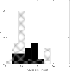
Figure 6: Histogram of the source sizes (deconvolved major axis) of the SMGs (solid) and control sample (cross-hatched) in the Lockman Hole.

Measuring the sizes of SMGs is crucial to understanding their formation. In the local universe, ULIRGs seem to be analogues of the high-redshift SMG population (Sanders & Mirabel, 1996). The most luminous of these are predominantly merger events and there is evidence that the similarly luminous high-redshift SMGs are also commonly undergoing mergers; physical associations are directly inferred from spectroscopy and multi-wavelength imaging (Ivison et al., 1998; Smail et al., 1998; Ivison et al., 2000; Conselice et al., 2003; Smail et al., 2004; Swinbank et al., 2004) whilst the double-peaked profiles often seen in mm-wave spectroscopy of the vast reservoirs of molecular gas (Frayer et al., 1998, 1999; Neri et al., 2003; Greve et al., 2005) are suggestive of orbital motions.

Tacconi et al. (2006) present observations at 1 and 3 mm of SMGs with the IRAM Plateau de Bure interferometer which at the shortest wavelength have a beamsize ($\sim$0.6 arcsec) that is similar to that of our MERLIN/VLA maps. They find that the SMGs (as seen in CO and/or mm-wave continuum emission) are generally compact; their sample of ten sources has a median size $\leq$0.5 arcsec ($\pm$0.1 arcsec). The sizes quoted by Tacconi et al. are ‘angular averaged’ and to facilitate a proper comparison with our data we plot the average of the major and minor axes of our SMGs in Fig. 7 along with the Tacconi et al. results. The two distributions appear similar, in both the position of the peaks and the range of sizes covered. A Kolmogorov-Smirnov (K-S) test (Press et al., 1992) gives a probability of 84 per cent that the differences between the two could arise by chance and thus strongly favours the null hypothesis that the two distributions are the same. This mirrors what is seen at much lower redshift, where the radio emission (Condon et al., 1991) and molecular gas (Downes & Solomon, 1998) have similar sizes.

Converting to linear distances for the SMGs with redshifts we find a range 1.2–7.7 kpc with a median of 4.9 kpc; Tacconi et al. (2006) measure a smaller, but similar, linear extent of $<$4 kpc. Given that the size of the central starburst in local ULIRGs is $\la$1 kpc, the high-redshift starbursts appear to be in general significantly larger, although the smallest (SMG06) is of comparable size to those seen at low redshift.

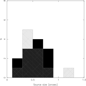
Figure 7: A comparison of the sizes of SMGs as measured by our MERLIN/VLA radio data (solid) and by Tacconi et al. (2006) in the mm waveband (cross-hatched).

Ivison et al. (2007) have explored the fraction of SMGs that contain multiple radio counterparts and find evidence that this is more common for the brighter sources, with separations between 2 and 6 arcsec. They are unable to probe below 2 arcsec due to the resolution of the VLA-only data, but despite the smaller beam of our combined MERLIN/VLA maps we see no examples of multiple sources with separations $<$2 arcsec. We can increase the resolution still further, at the expense of accurate imaging of extended emission, by examining the MERLIN-only maps. One of these, SMG10, reveals that a prominent extension in the MERLIN/VLA map contains a relatively high signal-to-noise ($\sim$6) component (Fig. 8). A two-Gaussian fit in jmfit gives a separation of 0.6 arcsec and a flux density ratio of $\sim$5:1. At the redshift of 1.212 this angular separation corresponds to a linear distance of $\sim$5 kpc. The nature of this second component is unknown and may be a radio jet, but it may also be a small-separation merger.

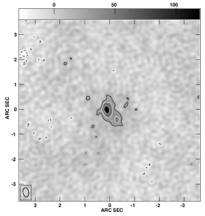
Figure 8: MERLIN-only map of SMG09 (LH 1200.008). The beam is shown in the bottom-left corner and has dimensions of $373\times 223$ mas² at a position angle of $9\aas@@fstack{\circ}7$. The greyscale has units of $\mu$Jy beam^-1 and contours are drawn at $-1$, 1, 2, 4, 8, etc. times the 3 $\sigma$ noise (3 $\times$ 8.5 $\mu$Jy beam^-1).

4.2 SMG sizes relative to the $\mu$Jy radio population

Also plotted in Fig. 6 are the major axes of the fits to the control sample, i.e. those $\mu$Jy radio sources which are not luminous in the submm waveband. The range of angular sizes for both samples is similar, covering approximately 0.1–1.4 arcsec although the median size of the control sample is formally smaller than that of the SMGs, 0.5 arcsec compared to 0.65 arcsec (with 1 $\sigma$ errors of about 0.1 arcsec). Another way of assessing the extension or otherwise of the two source populations is to compare the peak flux densities in the MERLIN-only and combined MERLIN/VLA maps. These ratios are plotted in Fig. 9 and a similar picture emerges; the control source distribution contains sources which are, in general, more compact. A K-S analysis gives low probabilities that the distributions are the same (30 and 17 per cent for the size and peak flux density plots, respectively).

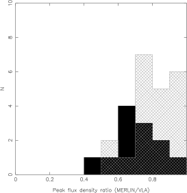
Figure 9: Histogram of the peak flux density ratio (MERLIN/VLA) of the SMGs (solid) and control sample (cross-hatched) in the Lockman Hole.

We plot the sizes of all our sources in Fig. 10 and include the bright source that was excluded from our control sample (a large, $\sim$4 arcsec, source which contains a radio core and two-sided jet). The distribution peaks strongly at angular extents in the range 0.4–0.6 arcsec. This is in apparent disagreement with Muxlow et al. (2005) and Chapman et al. (2004) who find that the average source size of $\mu$Jy radio sources is $\sim$1 arcsec and that there is a prominent tail extending to $\sim$4 arcsec. The Muxlow et al. data are also plotted in Fig. 10 so that the two samples can be easily compared; the two distributions are very different and they can formally be rejected as representing the same population with a K-S probability in excess of 99 per cent.

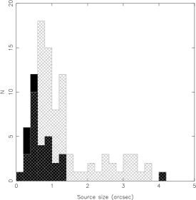
Figure 10: Histogram of the source sizes of our Lockman Hole sample as well as the faint radio population in the GOODS-N field of Muxlow et al. (2005). For the Lockman Hole (solid area) the sizes refer to the deconvolved major axis of a Gaussian fit whilst for GOODS-N (cross-hatched) it is the ‘largest angular size’.

The distributions in Fig. 10 differ in two ways. Firstly, the Lockman Hole data appear to consist of only a single source population, this being distributed approximately normally. The GOODS-N distribution is similar for the smaller sources, but peaks at a larger source size and has a significant tail out to angular extents of $\sim$4 arcsec. The absence of this tail in our sample (save for a single source) is particularly striking. Even taking into account possible errors in our model fitting (relatively weak extensions are not well modelled), we can be certain that only one source in our 12-arcmin-diameter field is larger than 2 arcsec.

The explanation for the difference in source size distributions in Fig. 10, especially with regard to the tail, is probably a combination of the larger sample and lower flux limit of Muxlow et al. (40 $\mu$Jy compared to our 50 $\mu$Jy) and cosmic variance. Our sources may also be smaller, particularly for sources in the population which peaks at around 0.5–1 arcsec, because of differences in the way the sizes were measured and also because we have attempted to remove the bandwidth smearing from our VLA data, something that was not done for the GOODS-N data.

5 Conclusions

We have presented sensitive maps (6 $\mu$Jy beam^-1 r.m.s.) of 12 SMGs in the Lockman Hole made from combined MERLIN and VLA data. This is the first time that wide-field (multi-channel) data from MERLIN and the VLA have been combined in the $(u,v)$ plane. The procedure to do this is straightforward, practical with modern desktop computing facilities and can be accomplished with existing software tools, i.e. aips.

From the radio morphology alone it has generally not been possible to determine unambiguously whether a source contains an AGN, except in one case which has a prominent jet (C19). In the local Universe, radio emission from most starburst galaxies is known to be concentrated in their galactic nuclei, so source compactness is no guarantee of an AGN. Indeed, even higher resolution – very long baseline interferometry – is required to improve our diagnostic ability, via sensitivity to more compact jets and via the ability to constrain the brightness temperature of unresolved emission to a regime unique to AGN.

Our maps have resolved the vast majority of the SMGs as well as a complementary sample of radio sources of similar flux density. A comparison of the properties of these two populations shows that the size distributions overlap considerably, but the SMGs are in general larger than the control sample (six of which harbour AGN, being luminous X-ray sources – see below). Even if some of our submm-luminous sources also contain significant emission from AGN, this suggests that the starburst component in high-redshift SMGs is extended and not confined to the nucleus.

This conclusion is strengthened by the measurement of similar sizes for the radio-emitting regions of SMGs and their molecular gas reservoirs, suggesting that AGN are not significantly contributing to the measured size of the radio emission. However, most high-redshift SMGs have much larger sizes (1.2–7.7 kpc) than local ULIRGs ($\leq$1 kpc), possibly the result of witnessing them at a less advanced stage of the merger process.

Despite our high resolution, as compared with the VLA, we find only one source that is resolved into multiple, distinct components. Determining the true nature of this source (and SMG06) – merger-induced starburst or AGN plus jet? – will require follow-up observations, but small separation ($<$2 arcsec) multiple counterparts to SMGs appear to be rare.

X-ray emission is a good indicator of AGN activity. Based on counterparts in the XMM-Newton catalogue of Brunner et al. (2007), we find a lower detection rate of X-ray luminous AGN amongst the submm-luminous sources than amongst the control sample (Poissonian probability, 89 per cent). Six of the control sources have a likely X-ray counterpart (C05, C10, C12, C13, C20 and C21) versus only one of the submm galaxies (SMG06). SMG06 is the hardest of the seven X-ray detections, consistent with enhanced X-ray absorption in a dust-obscured starburst (Page et al., 2004). It is also the most compact radio emitter amongst the SMGs, with a flat radio spectrum (Ivison et al., 2007).

$e$-MERLIN and the EVLA will soon be available, the broad-banded and hence much more sensitive versions of the current arrays. This will enable the $\mu$Jy radio population to be imaged at high resolution over larger areas and at increasingly faint flux limits. Also to come is the eSMA, a collaboration between the JCMT, the CSO and the telescopes of the Submillimeter Array. The resulting instrument will have a resolution at 345 GHz of 300 mas, extremely complementary to the angular scales being probed by the combined MERLIN and VLA maps presented in this paper. This will allow a direct comparison between the submm and radio morphologies of SMGs and we can thus examine the radio/far-IR correlation at unprecedented resolution.

References

- Alexander et al. (2003) Alexander D. M. et al., 2003, AJ, 125, 383
- Alexander et al. (2005) Alexander D. M., Bauer F. E., Chapman S. C., Smail I., Blain A. W., Brandt W. N., Ivison R. J., 2005, ApJ, 632, 736
- Biggs & Ivison (2006) Biggs A. D., Ivison R. J., 2006, MNRAS, 371, 963
- Brunner et al. (2007) Brunner H., Cappelluti N., Hasinger G., Barcons X., Fabian A. C., Mainieri V., Szokoly G., 2007, A&A, 711, astro-ph/0711.4822
- Chapman et al. (2003) Chapman S. C., Blain A. W., Ivison R. J., Smail I. R., 2003, Nat, 422, 695
- Chapman et al. (2005) Chapman S. C., Blain A. W., Smail I., Ivison R. J., 2005, ApJ, 622, 772
- Chapman et al. (2004) Chapman S. C., Smail I., Windhorst R., Muxlow T., Ivison R. J., 2004, ApJ, 611, 732
- Ciliegi et al. (2000) Ciliegi P., Zamorani G., Gruppioni C., Hasinger G., Lehmann I., Wilson G., 2000, in Plionis M., Georgantopoulos I., eds, Large Scale Structure in the X-ray Universe, Proceedings of the 20-22 September 1999 Workshop, Santorini, Greece. Atlantisciences, Paris, p. 347
- Condon et al. (1991) Condon J. J., Huang Z.-P., Yin Q. F., Thuan T. X., 1991, ApJ, 378, 65
- Conselice et al. (2003) Conselice C. J., Chapman S. C., Windhorst R. A., 2003, ApJ, 596, L5
- Coppin et al. (2006) Coppin K. et al., 2006, MNRAS, 372, 1621
- De Ruiter et al. (1997) De Ruiter H. R. et al., 1997, A&A, 319, 7
- Di Matteo et al. (2005) Di Matteo T., Springel V., Hernquist L., 2005, Nat, 433, 604
- Downes & Solomon (1998) Downes D., Solomon P. M., 1998, ApJ, 507, 615
- Egami et al. (2004) Egami E. et al., 2004, ApJS, 154, 130
- Fox et al. (2002) Fox M. J. et al., 2002, MNRAS, 331, 839
- Frayer et al. (1999) Frayer D. T. et al., 1999, ApJ, 514, L13
- Frayer et al. (1998) Frayer D. T., Ivison R. J., Scoville N. Z., Yun M., Evans A. S., Smail I., Blain A. W., Kneib J.-P., 1998, ApJ, 506, L7
- Garrett et al. (2001) Garrett M. A. et al., 2001, A&A, 366, L5
- Greve et al. (2005) Greve T. R. et al., 2005, MNRAS, 359, 1165
- Greve et al. (2004) Greve T. R., Ivison R. J., Bertoldi F., Stevens J. A., Dunlop J. S., Lutz D., Carilli C. L., 2004, MNRAS, 354, 779
- Häring & Rix (2004) Häring N., Rix H.-W., 2004, ApJ, 604, L89
- Hasinger et al. (2001) Hasinger G. et al., 2001, A&A, 365, L45
- Holland et al. (1999) Holland W. S. et al., 1999, MNRAS, 303, 659
- Huang et al. (2004) Huang J.-S. et al., 2004, ApJS, 154, 44
- Hughes et al. (1998) Hughes D. H. et al., 1998, Nat, 394, 241
- Ivison et al. (2007) Ivison R. J. et al., 2007, MNRAS, 380, 199
- Ivison et al. (2002) Ivison R. J. et al., 2002, MNRAS, 337, 1
- Ivison et al. (2000) Ivison R. J., Smail I., Barger A. J., Kneib J.-P., Blain A. W., Owen F. N., Kerr T. H., Cowie L. L., 2000, MNRAS, 315, 209
- Ivison et al. (2005) Ivison R. J. et al., 2005, MNRAS, 364, 1025
- Ivison et al. (1998) Ivison R. J., Smail I., Le Borgne J.-F., Blain A. W., Kneib J.-P., Bezecourt J., Kerr T. H., Davies J. K., 1998, MNRAS, 298, 583
- Laurent et al. (2005) Laurent G. T. et al., 2005, ApJ, 623, 742
- Laurent et al. (2006) Laurent G. T. et al., 2006, ApJ, 643, 38
- Lockman et al. (1986) Lockman F. J., Jahoda K., McCammon D., 1986, ApJ, 302, 432
- Lutz et al. (2005) Lutz D., Valiante E., Sturm E., Genzel R., Tacconi L. J., Lehnert M. D., Sternberg A., Baker A. J., 2005, ApJ, 625, L83
- Magorrian et al. (1998) Magorrian J. et al., 1998, AJ, 115, 2285
- Mainieri et al. (2002) Mainieri V., Bergeron J., Hasinger G., Lehmann I., Rosati P., Schmidt M., Szokoly G., Della Ceca R., 2002, A&A, 393, 425
- Marconi & Hunt (2003) Marconi A., Hunt L. K., 2003, ApJ, 589, L21
- Menéndez-Delmestre et al. (2007) Menéndez-Delmestre K. et al., 2007, ApJ, 655, L65
- Mortier et al. (2005) Mortier A. M. J. et al., 2005, MNRAS, 363, 563
- Muxlow et al. (2005) Muxlow T. W. B. et al., 2005, MNRAS, 358, 1159
- Neri et al. (2003) Neri R. et al., 2003, ApJ, 597, L113
- Page et al. (2004) Page M. J., Stevens J. A., Ivison R. J., Carrera F. J., 2004, ApJ, 611, L85
- Press et al. (1992) Press W. H., Teukolsky S. A., Vetterling W. T., Flannery B. P., 1992, Numerical recipes in FORTRAN. Cambridge Univ. Press, Cambridge
- Sanders & Mirabel (1996) Sanders D. B., Mirabel I. F., 1996, ARA&A, 34, 749
- Schwab (1984) Schwab F. R., 1984, AJ, 89, 1076
- Scott et al. (2002) Scott S. E. et al., 2002, MNRAS, 331, 817
- Silk & Rees (1998) Silk J., Rees M. J., 1998, A&A, 331, L1
- Smail et al. (2004) Smail I., Chapman S. C., Blain A. W., Ivison R. J., 2004, ApJ, 616, 71
- Smail et al. (1997) Smail I., Ivison R. J., Blain A. W., 1997, ApJ, 490, L5
- Smail et al. (1998) Smail I., Ivison R. J., Blain A. W., Kneib J.-P., 1998, ApJ, 507, L21
- Spergel et al. (2003) Spergel D. N. et al., 2003, ApJS, 148, 175
- Strom (2004) Strom R., 2004, in Bachiller R., Colomer F., Desmurs J.-F., de Vicente P., eds, European VLBI Network on New Developments in VLBI Science and Technology, p. 271
- Swinbank et al. (2004) Swinbank A. M., Smail I., Chapman S. C., Blain A. W., Ivison R. J., Keel W. C., 2004, ApJ, 617, 64
- Tacconi et al. (2006) Tacconi L. J. et al., 2006, ApJ, 640, 228
- Thompson et al. (1986) Thompson A. R., Moran J. M., Swenson G. W., 1986, Interferometry and synthesis in radio astronomy. Wiley-Interscience, New York