Dynamic Phase Transitions for Ferromagnetic Systems

Abstract.

This article presents a phenomenological dynamic phase transition theory for ferromagnetism, leading to a precise description of the dynamic transitions, and to a physical predication on the spontaneous magnetization. The analysis also suggests asymmetry of fluctuations in both the ferromagnetism and the PVT systems.

1. Introduction

Classically, phase transitions are classified by the Ehrenfest classification scheme, based on the lowest derivative of the free energy that is discontinuous at the transition. For ferromagnetic systems, it has been observed that the magnetization, which is the first derivative of the free energy with the applied magnetic field strength, increases continuously from zero as the temperature is lowered below the Curie temperature, and the magnetic susceptibility, the second derivative of the free energy with the field, changes discontinuously. Hence, the ferromagnetic phase transition in materials such as iron is regarded as a second order phase transition. However, a theoretical understanding of the transition is still lacking. The main objective of this article is to provide theoretical approach to dynamic phase transitions for ferromagnetic systems.

For the classical GL free energy, although both the steady state and time-dependent models provide some results in agreement with experiments, there are obvious discrepancies on both susceptibility and spontaneous magnetization. Hence a revised GL free energy is proposed and analyzed, leading to a precise description of the dynamic transitions, and to a physical predication on the spontaneous magnetization.

The analysis is based on the recently developed dynamic transition theory by the authors, together with a new dynamic classification scheme, which classifies phase transitions into three categories: Type-I, Type-II and Type-III, corresponding mathematically to continuous, jump, and mixed transitions, respectively; see Section 2 and the Appendix as well as two recent books by the authors [1, 3] for details.

We remark also that the analysis leads naturally to a physical conjecture on asymmetry of fluctuations, which appears in both the ferromagnetic system studied in this article and in PVT systems studied in [2].

This article is organized as follows. In Section 2, we review the dynamic classification scheme and the new time-dependent Ginzburg-Landau model for equilibrium phase transitions. Section 3 deals with the dynamic transition based on the classical Ginzburg-Landau energy, and Section 4 addresses the dynamic transition theory using a revised Ginzburg-Landau energy. Physical conclusions are given in Section 5, and dynamic transition theory is recapitulated in the Appendix.

2. General Principles of Phase Transition Dynamics

In this section, we recapitulate the new dynamic phase transition classification scheme to classify phase transitions into three categories: Type-I, Type-II and Type-III, corresponding mathematically to continuous, jump, and mixed transitions, respectively.

Then we recall a new time-dependent Ginzburg-Landau theory for modeling equilibrium phase transitions in statistical physics, derived based on the le Châtelier principle and some mathematical insights on pseudo-gradient systems.

Both the classification scheme and the Ginzburg-Landau theory was developed recently by the authors, and we refer interested readers to [1, 3, 2] for details.

2.1. Dynamic classification scheme

In sciences, nonlinear dissipative systems are generally governed by differential equations, which can be expressed in the following abstract form

(2.1) $$\left.\begin{aligned} &\frac{du}{dt}=L_{\lambda}u+G(u,\lambda),\\ &u(0)=\varphi,\end{aligned}\right.$$

where $u:[0,\infty)\rightarrow X$ is the unknown function, $\lambda\in\mathbb{R}^{N}$ $(N\geq 1)$ is the control parameter, $X$ and $X_{1}$ are two Banach spaces with $X_{1}\subset X$ being a dense and compact inclusion, $L_{\lambda}=-A+B_{\lambda}$ and $G(\cdot,\lambda):X_{1}\rightarrow X$ are $C^{r}(r\geq 0)$ mappings depending continuously on $\lambda$, $L_{\lambda}:X_{1}\rightarrow X$ is a sectorial operator, and

(2.2) $$\left.\begin{aligned} &A:X_{1}\rightarrow X&&\text{a\ linear\ homeomorphism},\\ &B_{\lambda}:X_{1}\rightarrow X&&\text{a\ linear\ compact\ operator}.\end{aligned}\right.$$

In following, we introduce some basic and universal concepts in nonlinear sciences.

First, a state of the system (2.1) at $\lambda$ is usually referred to as a compact invariant set $\Sigma_{\lambda}$. In many applications, $\Sigma_{\lambda}$ is a singular point or a periodic orbit. A state $\Sigma_{\lambda}$ of (2.1) is stable if $\Sigma_{\lambda}$ is an attractor, otherwise $\Sigma_{\lambda}$ is called unstable.

Second, we say that the system (2.1) has a phase transition from a state $\Sigma_{\lambda}$ at $\lambda=\lambda_{0}$ if $\Sigma_{\lambda}$ is stable on $\lambda<\lambda_{0}$ (or on $\lambda>\lambda_{0}$) and is unstable on $\lambda>\lambda_{0}$ (or on $\lambda<\lambda_{0}$). The critical parameter $\lambda_{0}$ is called a critical point. In other words, the phase transition corresponds to an exchange of stable states.

The concept of phase transition originates from the statistical physics and thermodynamics. In physics and chemistry, ”phase” means the homogeneous part in a heterogeneous system. However, here the so called phase means the stable state in the systems of nonlinear sciences including physics, chemistry, biology, ecology, economics, fluid dynamics and geophysical fluid dynamics, etc. Hence, here the content of phase transition has been endowed with more general significance. In fact, the phase transition dynamics introduced here can be applied to a wide variety of topics involving the universal critical phenomena of state changes in nature in a unified mathematical viewpoint and manner.

Third, if the system (2.1) possesses the gradient-type structure, then the phase transitions are called equilibrium phase transition; otherwise they are called the non-equilibrium phase transitions.

Fourth, classically, there are several ways to classify phase transitions. The one most used is the Ehrenfest classification scheme, which groups phase transitions based on the degree of non-analyticity involved. First order phase transitions are also called discontinuous, and higher order phase transitions $(n>1)$ are called continuous.

Here we introduce the following notion of dynamic classification scheme:

Definition 2.1.

Let $\lambda_{0}\in\mathbb{R}^{N}$ be a critical point of (2.1), and (2.1) undergo a transition from state $\Sigma^{1}_{\lambda}$ to $\Sigma^{2}_{\lambda}$. There are three types of phase transitions for (2.1) at $\lambda=\lambda_{0}$, depending on their dynamic properties: continuous, jump, and mixed as given in Theorem A.1, which are called Type-I, Type-II and Type-III respectively.

The main characteristics of Type-II phase transitions is that there is a gap between $\Sigma^{1}_{\lambda}$ and $\Sigma^{2}_{\lambda}$ at the critical point $\lambda_{0}$. In thermodynamics, the metastable states correspond in general to the super-heated or super-cooled states, which have been found in many physical phenomena. In particular, Type-II phase transitions are always accompanied with the latent heat to occur.

In a Type-I phase transition, two states $\Sigma^{1}_{\lambda}$ and $\Sigma^{2}_{\lambda}$ meet at $\lambda_{0}$, i.e., the system undergoes a continuous transition from $\Sigma^{1}_{\lambda}$ to $\Sigma^{2}_{\lambda}$.

In a Type-III phase transition, there are at least two different stable states $\Sigma^{\lambda}_{2}$ and $\Sigma^{\lambda}_{3}$ at $\lambda_{0}$, and system undergoes a continuous transition to $\Sigma^{\lambda}_{2}$ or a jump transition to $\Sigma^{\lambda}_{3}$, depending on the fluctuations.

It is clear that a Type-II phase transition of gradient-type systems must be discontinuous or the zero order because there is a gap between $\Sigma^{1}_{\lambda}$ and $\Sigma^{j}_{\lambda}$ $(2\leq j\leq K)$. For a Type-I phase transition, the energy is continuous, and consequently, it is an $n$-th order transition in the Ehrenfest sense for some $n\geq 2$. A Type-III phase transition is indefinite, for the transition from $\Sigma^{1}_{\lambda}$ to $\Sigma^{2}_{\lambda}$ it may be continuous, i.e., $dF^{-}/d\lambda=dF^{+}_{2}/d\lambda$, and for the transitions from $\Sigma^{1}_{\lambda}$ to $\Sigma^{3}_{\lambda}$ it may be discontinuous: $dF^{-}/d\lambda\neq dF^{+}_{3}/d\lambda$ at $\lambda=\lambda_{0}$.

2.2. Time-dependent Ginzburg-Landau models for equilibrium phase transitions

In this subsection, we introduce the time-dependent Ginzburg-Landau model for equilibrium phase transitions.

We start with thermodynamic potentials and the Ginzburg-Landau free energy. As we know, four thermodynamic potentials– internal energy, the enthalpy, the Helmholtz free energy and the Gibbs free energy–are useful in the chemical thermodynamics of reactions and non-cyclic processes.

Consider a thermal system, its order parameter $u$ changes in $\Omega\subset\mathbb{R}^{n}$ $(1\leq n\leq 3)$. In this situation, the free energy of this system is of the form

(2.3) $${\mathcal{H}}(u,\lambda)={\mathcal{H}}_{0}+\int_{\Omega}\Big{[}\frac{1}{2}\sum^{m}_{i=1}\mu_{i}|\nabla u_{i}|^{2}+g(u,\nabla u,\lambda)\Big{]}dx$$

where $N\geq 3$ is an integer, $u=(u_{1},\cdots,u_{m}),\mu_{i}=\mu_{i}(\lambda)>0$, and $g(u,\nabla u,\lambda)$ is a $C^{r}(r\geq 2)$ function of $(u,\nabla u)$ with the Taylor expansion

(2.4) $$g(u,\nabla u,\lambda)=\sum\alpha_{ijk}u_{i}D_{j}u_{k}+\sum^{N}_{|I|=1}\alpha_{I}u^{I}+o(|u|^{N})-fX,$$

where $I=(i_{1},\cdots,i_{m}),i_{k}\geq 0$ are integer, $|I|=\sum^{m}_{k=1}i_{k}$, the coefficients $\alpha_{ijk}$ and $\alpha_{I}$ continuously depend on $\lambda$, which are determined by the concrete physical problem, $u^{I}=u^{i_{1}}_{1}\cdots u^{im}_{m}$ and $fX$ the generalized work.

Thus, the study of thermal equilibrium phase transition for the static situation is referred to the steady state bifurcation of the system of elliptic equations

$$\left.\begin{aligned} &\frac{\delta}{\delta u}{\mathcal{H}}(u,\lambda)=0,\\ &\frac{\partial u}{\partial n}|_{\partial\Omega}=0,\ \ \ \ (\text{or}\ u|_{\partial\Omega}=0),\end{aligned}\right.$$

where $\delta/\delta u$ is the variational derivative.

A thermal system is controled by some parameter $\lambda$. When $\lambda$ is for from the critical point $\lambda_{0}$ the system lies on a stable equilibrium state $\Sigma_{1}$, and when $\lambda$ reaches or exceeds $\lambda_{0}$ the state $\Sigma_{1}$ becomes unstable, and meanwhile the system will undergo a transition from $\Sigma_{1}$ to another stable state $\Sigma_{2}$. The basic principle is that there often exists fluctuations in the system leading to a deviation from the equilibrium states, and the phase transition process is a dynamical behavior, which should be described by a time-dependent equation.

To derive a general time-dependent model, first we recall that the classical le Châtelier principle amounts to saying that for a stable equilibrium state of a system $\Sigma$, when the system deviates from $\Sigma$ by a small perturbation or fluctuation, there will be a resuming force to retore this system to return to the stable state $\Sigma$. Second, we know that a stable equilibrium state of a thermal system must be the minimal value point of the thermodynamic potential.

By the mathematical characterization of gradient systems and the le Châtelier principle, for a system with thermodynamic potential ${\mathcal{H}}(u,\lambda)$, the governing equations are essentially determined by the functional ${\mathcal{H}}(u,\lambda)$. When the order parameters $(u_{1},\cdots,u_{m})$ are nonconserved variables, i.e., the integers

$$\int_{\Omega}u_{i}(x,t)dx=a_{i}(t)\neq\text{constant}.$$

then the time-dependent equations are given by

(2.5) $$\left.\begin{aligned} &\frac{\partial u_{i}}{\partial t}=-\beta_{i}\frac{\delta}{\delta u_{i}}{\mathcal{H}}(u,\lambda)+\Phi_{i}(u,\nabla u,\lambda),\\ &\frac{\partial u}{\partial n}|_{\partial\Omega}=0\ \ \ \ (\text{or}\ u|_{\partial\Omega}=0),\\ &u(x,0)=\varphi(x),\end{aligned}\right.$$

for any $1\leq i\leq m$, where $\delta/\delta u_{i}$ are the variational derivative, $\beta_{i}>0$ and $\Phi_{i}$ satisfy

(2.6) $$\int_{\Omega}\sum_{i}\Phi_{i}\frac{\delta}{\delta u_{i}}{\mathcal{H}}(u,\lambda)dx=0.$$

The condition (2.6) is required by the Le Châtelier principle. In the concrete problem, the terms $\Phi_{i}$ can be determined by physical laws and (2.6).

When the order parameters are the number density and the system has no material exchange with the external, then $u_{j}$ $(1\leq j\leq m)$ are conserved, i.e.,

(2.7) $$\int_{\Omega}u_{j}(x,t)dx=\text{constant}.$$

This conservation law requires a continuous equation

(2.8) $$\frac{\partial u_{j}}{\partial t}=-\nabla\cdot J_{j}(u,\lambda),$$

where $J_{j}(u,\lambda)$ is the flux of component $u_{j}$. In addition, $J_{j}$ satisfy

(2.9) $$J_{j}=-k_{j}\nabla(\mu_{j}-\sum_{i\neq j}\mu_{i}),$$

where $\mu_{l}$ is the chemical potential of component $u_{l}$,

(2.10) $$\mu_{j}-\sum_{i\neq j}\mu_{i}=\frac{\delta}{\delta u_{j}}{\mathcal{H}}(u,\lambda)-\phi_{j}(u,\nabla u,\lambda),$$

and $\phi_{j}(u,\lambda)$ is a function depending on the other components $u_{i}$ $(i\neq j)$. When $m=1$, i.e., the system consists of two components $A$ and $B$, this term $\phi_{j}=0$. Thus, from (2.8)-(2.10) we obtain the dynamical equations as follows

(2.11) $$\left.\begin{aligned} &\frac{\partial u_{j}}{\partial t}=\beta_{j}\Delta\left[\frac{\delta}{\delta u_{j}}{\mathcal{H}}(u,\lambda)-\phi_{j}(u,\nabla u,\lambda)\right],\\ &\frac{\partial u}{\partial n}|_{\partial\Omega}=0,\ \ \ \ \frac{\partial\Delta u}{\partial n}|_{\partial\Omega}=0,\\ &u(x,0)=\varphi(x),\end{aligned}\right.$$

for $1\leq j\leq m$, where $\beta_{j}>0$ are constants, $\phi_{j}$ satisfy

(2.12) $$\int_{\Omega}\sum_{j}\Delta\phi_{j}\cdot\frac{\delta}{\delta u_{j}}{\mathcal{H}}(u,\lambda)dx=0.$$

If the order parameters $(u_{1},\cdots,u_{k})$ are coupled to the conserved variables $(u_{k+1},\cdots,u_{m})$, then the dynamical equations are

(2.13) $$\left.\begin{aligned} &\frac{\partial u_{i}}{\partial t}=-\beta_{i}\frac{\delta}{\delta u_{i}}{\mathcal{H}}(u,\lambda)+\Phi_{i}(u,\nabla u,\lambda),\\ &\frac{\partial u_{j}}{\partial t}=\beta_{j}\Delta\left[\frac{\delta}{\delta u_{j}}{\mathcal{H}}(u,\lambda)-\phi_{j}(u,\nabla u,\lambda)\right],\\ &\frac{\partial u_{i}}{\partial n}|_{\partial\Omega}=0\ \ \ \ (\text{or}\ u_{i}|_{\partial\Omega}=0),\\ &\frac{\partial u_{j}}{\partial n}|_{\partial\Omega}=0,\ \ \ \ \frac{\partial\Delta u_{j}}{\partial n}|_{\partial\Omega}=0,\\ &u(x,0)=\varphi(x).\end{aligned}\right.$$

for $1\leq i\leq k$ and $k+1\leq j\leq m$.

The model (2.13) gives a general form of the governing equations to thermodynamic phase transitions. Hence, the dynamics of equilibrium phase transition in statistic physics is based on the new Ginzburg-Landau formulation (2.13).

Physically, the initial value condition $u(0)=\varphi$ in (2.13) stands for the fluctuation of system or perturbation from the external. Hence, $\varphi$ is generally small. However, we can not exclude the possibility of a bigger noise $\varphi$.

From conditions (2.6) and (2.12) it follows that a steady state solution $u_{0}$ of (2.13) satisfies

(2.14) $$\left.\begin{aligned} &\Phi_{i}(u_{0},\nabla u_{0},\lambda)=0&&\forall 1\leq i\leq k,\\ &\Delta\phi_{j}(u_{0},\nabla u_{0},\lambda)=0&&\forall k+1\leq j\leq m.\end{aligned}\right.$$

Hence a stable equilibrium state must reach the minimal value of thermodynamic potential. In fact, $u_{0}$ fulfills

(2.15) $$\left.\begin{aligned} &\beta_{i}\frac{\delta}{\delta u_{i}}{\mathcal{H}}(u_{0},\lambda)-\Phi_{i}(u_{0},\nabla u_{0},\lambda)=0,\\ &\beta_{j}\Delta\frac{\delta}{\delta u_{j}}{\mathcal{H}}(u_{0},\lambda)-\Delta\phi_{j}(u_{0},\nabla u_{0},\lambda)=0,\\ &\frac{\partial u_{i}}{\partial n}|_{\partial\Omega}=0\ \ \ \ (\text{or}\ u_{i}|_{\partial\Omega}=0),\\ \\ &\frac{\partial u_{j}}{\partial n}|_{\partial\Omega}=0,\ \ \ \ \frac{\partial\Delta u_{j}}{\partial n}|_{\partial\Omega}=0,\end{aligned}\right.$$

for $1\leq i\leq k$ and $k+1\leq j\leq m$. Multiplying $\Phi_{i}(u_{0},\nabla u_{0},\lambda)$ and $\phi_{j}(u_{0},\nabla u_{0},\lambda)$ on the first and the second equations of (2.15) respectively, and integrating them, then we infer from (2.6) and (2.12) that

$$\int_{\Omega}\sum_{i}\Phi^{2}_{i}(u_{0},\nabla u_{0},\lambda)dx=0,$$

$$\int_{\Omega}\sum_{j}|\nabla\phi_{j}(u_{0},\nabla u_{0},\lambda)|^{2}dx=0,$$

which imply that (2.14) holds true.

3. Classical Theory of Ferromagnetism

A ferromagnetic material consists of lattices containing particles with a magnetic moment. When no external field is present and the temperature is above some critical value, called the Curie temperature, the magnetic moments are oriented at random and there is no net magnetization. However, as the temperature is lowered, magnetic interaction energy between lattice sites becomes more important than the random thermal energy. Below the Curie temperature, the magnetic moments become ordered in the space and a spontanous magnetization appears. The phase transition from a paramagnetic to a ferromagnetic system takes place at the Curie Temperature.

The phase diagrams for magnetic systems are given in Figures 3.1-3.3. In Figure 3.1, below the Curie temperature, the magnetization occurs spontaneously, and the zero magnetic field $H=0$ separates the two possible orientations of magnetization. Figure 3.2 provides a sketch of the isotherms of magnetic system, and Figure 3.3 gives the magnetization as a function of temperature; see also Reichl [5] and Onuki [4] for details.

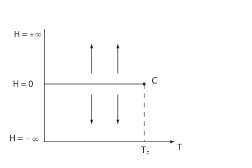
Figure 3.1. Below the Curie point the magnetization occurs spontaneously; the curve $H=0$ separates the two possible orientations of magnetization.

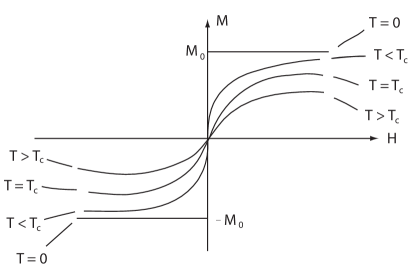
Figure 3.2. A sketch of the isotherms for a magnetic system.

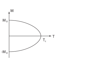
Figure 3.3. A sketch of the spontaneous magnetization of a magnetic system.

Based on the classical Ginzburg-Landau theory, for an isotropic system, the Helmholtz free energy can be expressed as

$$A(M,T)=A_{0}(T)+\frac{1}{2}\alpha_{2}(T)|M|^{2}+\frac{1}{4}\alpha_{4}(T)|M|^{4}+\cdots,$$

where $A_{0}(T)$ is a magnetization-independent contribution to the free energy, $|M|^{2}=M\cdot M$, and $M=(M_{1},M_{2},M_{3})$ is the magnetization of the system. When an external field $H$ is present, the Gibbs free energy is given by

$$G(M,H,T) = A(M,T)-H\cdot M$$

$$= A_{0}(T)-H\cdot M+\frac{1}{2}\alpha_{2}(T,H)|M|^{2}+\frac{1}{4}\alpha_{4}(T,H)|M|^{4}+\cdots.$$

For small $H$, $\alpha_{2}$ and $\alpha_{4}$ can be considered to be independent of $H$, and near the Curie point $T_{c}$ we have

$$\alpha_{2}(T)=\alpha_{0}(T-T_{c}),\ \ \ \ \alpha_{4}(T)>0.$$

Usually, $G(M,H,T)$ is called the Ginzburg-Landau free energy. To omit the higher order terms than $|M|^{4}$, it is known that the equilibrium state $M$ of the ferromagnetic system satisfies

(3.1) $$\frac{\delta}{\delta M}G=\alpha_{4}|M|^{2}M+\alpha_{2}M-H=0.$$

Thus above the Curie point we obtain from (3.1) that

(3.2) $$\left.\begin{aligned} &M\simeq\frac{1}{\alpha_{2}}H,\\ &\chi=\frac{\partial M}{\partial H}=\frac{1}{\alpha_{2}(T)}=\frac{1}{\alpha_{0}(T-T_{c})},\end{aligned}\right.$$

where $\chi$ is the isothermal susceptibility, which is a scalar because the system is isotropic. Below the critical point, for $H=0$, the magnetization $M$ obeys

(3.3) $$|M|=\sqrt{\frac{\alpha_{0}(T_{c}-T)}{\alpha_{4}}},\qquad\frac{\partial|M|}{\partial T}=-\frac{1}{2}\sqrt{\frac{\alpha_{0}}{\alpha_{4}(T_{c}-T)}}.$$

The heat capacity at $T=T_{c}$ is

(3.4) $$C(T<T_{c})-C(T>T_{c})= -T\frac{\partial^{2}G}{\partial T^{2}}\Big{|}_{T=T_{c}}$$

$$= -T_{c}\frac{\partial^{2}}{\partial T^{2}}\left(\frac{1}{2}\alpha_{2}|M|^{2}+\frac{1}{4}\alpha_{4}|M|^{4}\right)\Big{|}_{T=T_{c}}$$

$$= \frac{\alpha^{2}_{0}T_{c}}{2\alpha_{4}}.$$

We infer then from (3.2)-(3.4) the following classical conclusions for an isotropic magnetic system:

• When as external magnetic field is present, a nonzero magnetization exists above the Curie point $T_{c}$, which has the same direction as the applied field $H$.

• Near the critical point $T_{c}$ the susceptibility $\chi$ tends to infinite with the rate $(T-T_{c})^{-1}$, i.e., a very small applied field at $T=T_{c}$ can yield a large effect on the magnetization.

• In the absence of an external field (i.e., $H=0)$, below the critical point a spontaneous magnetization $M$ appears, which depends continuously on $T$ and tends to zero with the rate $(T-T_{c})^{{1}/{2}}$; namely the transition is of the second order.

• The heat capacity at $T=T_{c}$ has a jump with the gap $\Delta C=\frac{\alpha^{2}_{0}T_{c}}{2\alpha_{4}}$, and the jump has the shape of a $\lambda$, as shown in Figure 3.4.

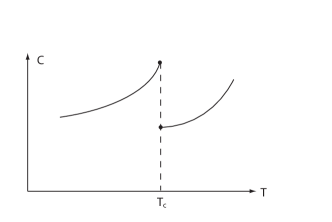
Figure 3.4.

Qualitatively, part of the above conclusions are in agreement with experimental results.

However these conclusions lead to wrong susceptibility and spontaneous magnetization, whose experimental rates are given by $\chi\propto(T-T_{c})^{-r}$ with $r=1.3$, and by $M\propto(T-T_{c})^{\beta}$ with $\beta={1}/{3}$.

Free energy $G$ must be a function of the magnetization $M$. Hence the errors are originated from the fact that the expression of $G$ in the Ginzburg-Landau theory is an approximation. It is difficult to derive a precise formula because $G$ is not analytic on $|M|$, even the differentibility of $G$ on $|M|$ is very low.

If we study the dynamical properties of ferromagnetic systems by using the classical Ginzburg-Landau free energy, we shall see a more serious error when an external field is present.

To see this, the dynamic equation of classical theory is given by

(3.5) $$\frac{dM}{dt}=-\alpha_{2}M-\alpha_{4}|M|^{2}M+H.$$

For simplicity, we take $H=(h,0,0)$ with $h>0$, it is equivalent that we take the $x_{1}$-axis in the direction of $H$. Then the equation

$$\alpha_{4}|M|^{2}M+\alpha_{2}M-H=0$$

has a steady state solution $M_{0}=(m_{0},0,0)$ for $T\geq 0$, which is the magnetization induced by $H$. Make the transformation

$$M=M^{\prime}+M_{0}.$$

Then, the equation (3.5) is rewritten as (drop the primes)

(3.6) $$\left.\begin{aligned} &\frac{dM_{1}}{dt}=-(\alpha_{2}+3\alpha_{4}m^{2}_{0})M_{1}-2\alpha_{4}m_{0}M^{2}_{1}-\alpha_{4}m_{0}|M|^{2}-\alpha_{4}|M|^{2}M_{1},\\ &\frac{dM_{2}}{dt}=-(\alpha_{2}+\alpha_{4}m^{2}_{0})M_{2}-2\alpha_{4}m_{0}M_{1}M_{2}-\alpha_{4}|M|^{2}M_{2},\\ &\frac{dM_{3}}{dt}=-(\alpha_{2}+\alpha_{4}m^{2}_{0})M_{3}-2\alpha_{4}m_{0}M_{1}M_{3}-\alpha_{4}|M|^{2}M_{3}.\end{aligned}\right.$$

Comparing the two critical parameter curves

$$\alpha_{2}+3\alpha_{4}m^{2}_{0}=2 \Rightarrow T_{1}=T_{c}-3\alpha_{4}m^{2}_{0}/\alpha_{0},$$

$$\alpha_{2}+\alpha_{4}m^{2}_{0}=0 \Rightarrow T_{2}=T_{c}-\alpha_{4}m^{2}_{0}/\alpha_{0},$$

we find that $T_{2}>T_{1}$. By Theorem A.1, (3.6) has the first transition at $T=T_{2}$, where a new magnetization $M=(M_{1},M_{2},M_{3})$, with $M_{2}\not=0$ and $M_{3}\not=0$, appears. This is unrealistic because any magnetization $M$ of this system must have the same direction as $H=(h,0,0)$; see Figure 3.1.

In fact, when a magnetic field $H$ is applied on an isotropic system the direction of $H$ is a favorable one for magnetization. However, in (3.5) this point is not manifested. Therefore, to investigate the phase transition dynamics of ferromagnetic systems we need to revise the $GL$ free energy.

4. Dynamic Transitions in Ferromagnetism

4.1. Revised Ginzburg-Landau free energy

Let the ferromagnetic system be isotropic. When a magnetic field $H$ is present, we introduce a second order symmetric tensor

$$A(T,H)=(a_{ij}(T,H)),\ \ \ \ a_{ij}=a_{ji},\ \ \ \ 1\leq i,\ j\leq 3,$$

such that $A(T,0)=0$, and $A(T,H)$ has eigenvalues

$$\lambda_{1}=\lambda_{1}(T,H),\ \ \ \ \lambda_{2}=\lambda_{3}=0,\ \ \ \ \text{with}\ \lambda_{1}(T,H)>0\ \text{as}\ H\neq 0,$$

and $H$ is the eigenvector of $A$ corresponding to $\lambda_{1}$:

(4.1) $$AH=\lambda_{1}H\ \ \ \ (\lambda_{1}>0\ \text{as}\ H\neq 0,\ \ \ \ \lambda_{1}=0\ \text{as}\ H=0).$$

It is clear that if we take the coordinate system $(x_{1},x_{2},x_{3})$ with $x_{1}$-axis in the $H$-direction, then $H=(H_{1},0,0)$ and

(4.2) $$A=\left(\begin{matrix}\lambda_{1}&0&0\\ 0&0&0\\ 0&0&0\end{matrix}\right).$$

Physically, condition (4.1) means that $H$ is a favorable direction of magnetization if we add a term

$$-MAM^{T}=-\sum a_{ij}M_{i}M_{j}$$

in the free energy. We also need to consider the nonlinear effect acted by $H$. To this end we introduce the term $-|M|^{2}M\cdot H$ in the free energy.

Thus when the applied field $H$ may vary in $\Omega\subset\mathbb{R}^{n}$ $(n=2,3)$, then the $GL$ free energy is in the form

(4.3) $$G(M,T,H)=G_{0} +\frac{1}{2}\int_{\Omega}\Big{[}\mu|\nabla M|^{2}+\alpha_{2}|M|^{2}+\frac{\alpha_{4}}{2}|M|^{4}$$

$$-\sum a_{ij}M_{i}M_{j}-f(T,H,M)M\cdot H\Big{]}dx,$$

where $G_{0}=G_{0}(T)$ is independent of $M$ and $H$, and $f$ is a scalar function of $T,H$ and $M$, defined by

(4.4) $$f(T,H,M)=2(1+\beta|M|^{2}),\qquad\beta=\beta(T,H)>0.$$

For $\alpha_{2}$ and $\alpha_{4}$ we assume that

(4.5) $$\alpha_{2}=\alpha_{0}(H)(T-T_{0}(H)),\ \ \ \ T_{0}(0)=T_{c},\ \ \ \ \alpha_{0}>0,\ \ \ \ \alpha_{4}>0.$$

By the standard model (2.5), we derive from (4.3) and (4.4) the following dynamical equations:

(4.6) $$\frac{\partial M_{i}}{\partial t}= \mu\Delta M_{i}-\alpha_{2}M_{i}+\sum^{3}_{j=1}a_{ij}M_{j}-\alpha_{4}|M|^{2}M_{i}$$

$$+\beta|M|^{2}H_{i}+2\beta(M\cdot H)M_{i}+H_{i} \text{for }1\leq i\leq 3.$$

The boundary condition is given by

(4.7) $$\left.\frac{\partial M}{\partial n}\right|_{\partial\Omega}=0.$$

Obviously, if $H=0$, (4.6) coincide with the classical equations. For simplicity, hereafter we always take

(4.8) $$H=(h,0,0)\qquad(h>0\ \text{is a constant}).$$

When $H$ is constant, in the study of phase transitions of magnetic systems, (4.6) can be replaced by a system of ordinary differential equations as follows:

(4.9) $$\left.\begin{aligned} &\frac{dM_{1}}{dt}=(\lambda_{1}-\alpha_{2})M_{1}+\beta h|M|^{2}+2\beta hM^{2}_{1}-\alpha_{4}|M|^{2}M_{1}+h,\\ &\frac{dM_{2}}{dt}=-\alpha_{2}M_{2}+2\beta hM_{1}M_{2}-\alpha_{4}|M|^{2}M_{2},\\ &\frac{dM_{3}}{dt}=-\alpha_{2}M_{3}+2\beta hM_{1}M_{3}-\alpha_{4}|M|^{2}M_{3}.\end{aligned}\right.$$

Equations (4.9) have a steady state solution induced by $H$:

$$M^{*}=(m_{0},0,0),\ \ \ \ \text{with}\ \lim_{h\to 0}m_{0}=0.$$

We see in Figure 3.2 that the magnetization $M^{*}$ has an upper bound. Namely there is an $M_{0}$ such that

(4.10) $$\left.\begin{aligned} &|M^{*}|<|M_{0}|&&\qquad\forall H\in\mathbb{R}^{3},\ \ \ \ T\geq 0,\\ &M^{*}\rightarrow M_{0}&&\qquad\text{if }h\rightarrow\infty.\end{aligned}\right.$$

To satisfy (4.10) it is necessary to assume that the coefficients $\alpha_{0}$ and $\alpha_{4}$ as in (4.5) possess the properties

(4.11) $$\alpha_{0}(H)\rightarrow+\infty,\ \ \ \ \alpha_{4}(T,H)\rightarrow+\infty,\ \ \ \ \text{as}\ h\rightarrow\infty.$$

Both conditions (4.5) and (4.11) are physical.

4.2. Dynamic transitions

In this subsection, to illustrate the main ideas, we only consider the case where $H$ is a constant on $\Omega$. Therefore we shall study phase transition dynamics of the ferromagnetic systems by using equations (4.9) for $h>0$. Analysis for more general case can be carried out in the same fashion, and will be reported elsewhere.

Take the transformation in (4.9)

(4.12) $$M=M^{*}+M^{\prime}.$$

Then equations (4.9) are rewritten as (drop the primes)

(4.13) $$\left.\begin{aligned} &\frac{dM_{1}}{dt}=\beta_{1}M_{1}-2a_{2}M^{2}_{1}-a_{2}|M|^{2}-\alpha_{4}|M|^{2}M_{1},\\ &\frac{dM_{2}}{dt}=\beta_{2}M_{2}-2a_{2}M_{1}M_{2}-\alpha_{4}|M|^{2}M_{2},\\ &\frac{dM_{3}}{dt}=\beta_{2}M_{3}-2a_{2}M_{1}M_{3}-\alpha_{4}|M|^{2}M_{3},\end{aligned}\right.$$

where

$$a_{2}=\alpha_{4}m_{0}-\beta h,$$

$$\beta_{1}=\lambda_{1}+6\beta hm_{0}-3\alpha_{4}m^{2}_{0}-\alpha_{2},$$

$$\beta_{2}=2\beta hm_{0}-\alpha_{4}m^{2}_{0}-\alpha_{2}.$$

The critical parameter curves $\beta_{1}=0$ and $\beta_{2}=0$ are given by

$$\beta_{1}=0\Rightarrow T_{1}=T_{0}(H)+\frac{1}{\alpha_{0}}(\lambda_{1}+6\beta hm_{0}-3\alpha_{4}m^{2}_{0}),$$

$$\beta_{2}=0\Rightarrow T_{2}=T_{0}(H)+\frac{1}{\alpha_{0}}(2\beta hm_{0}-\alpha_{4}m^{2}_{0}).$$

It is clear that $T_{1}>T_{2}$ provided

(4.14) $$\lambda_{1}>2m_{0}(\alpha_{4}m_{0}-2\beta h),\ \ \ \ \text{for}\ h>0.$$

Therefore, under condition (4.14), the equations (4.13) have a transition at $T=T_{1}$ in the space

(4.15) $$E=\{(M_{1},0,0)|\ -\infty<M_{1}<\infty\}.$$

More precisely, we have the following transition theorem.

Theorem 4.1.

Assume the condition (4.14) and $a_{2}\neq 0$. Then (4.13) has a Type-III (mixed) transition at $T=T_{1}$, and the transition occurs in the space $E$. The phase diagram is as shown in Figure 4.1. Moreover we have the following assertions:

• There are two stable equilibrium states near $T=T_{1}$, which are given by

  $$M^{+}_{1}=\left\{\begin{aligned} &0&&\text{if }T>T_{1},\\ &\frac{1}{2\alpha_{4}}[-3a_{2}+\sqrt{9a^{2}_{2}+4\alpha_{4}\beta_{1}}]&&\text{if }T<T_{1},\end{aligned}\right.$$

  $$M^{-}_{1}=-\frac{1}{2\alpha_{4}}[3a_{2}+\sqrt{9a^{2}_{2}+4\alpha_{4}\beta_{1}}].$$

• If $T<T_{1}$, $M^{+}_{1}$ is stable in the region $0<M_{1}<\infty$, and $M^{-}_{1}$ is stable in $-\infty<M_{1}<0$.

• If $T>T_{1}$, $M^{+}_{1}=0$ is stable in $-b<M_{1}<\infty$ and $M^{-}_{1}$ is stable in $-\infty<M_{1}<-b$, where

  $$b=\frac{1}{2\alpha_{4}}[3a_{2}-\sqrt{9a^{2}_{2}+4\alpha_{4}\beta_{1}}]>0\qquad\text{ for }T>T_{1}.$$

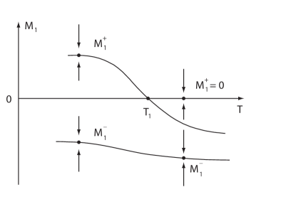
Figure 4.1.

Proof.

It is clear that if (4.14) holds, then

$$\beta_{1}(T)\left\{\begin{aligned} &<0&&\text{ if }T>T_{1},\\ &=0&&\text{ if }T=T_{1},\\ &>0&&\text{ if }T<T_{1},\end{aligned}\right.$$

$$\beta_{2}(T_{1})<0.$$

Hence, by Theorem A.1 the system (4.13) has a transition at $T=T_{1}$. Obviously, the space $E$ defined by (4.15) is the center manifold of (4.13) near $T=T_{1}$. Hence, the reduced equation of (4.13) on $E$ is expressed as

(4.16) $$\frac{dM_{1}}{dt}=\beta_{1}M_{1}-3a_{2}M^{2}_{1}-\alpha_{4}M^{3}_{1}.$$

As $a_{2}\neq 0$, by Theorem A.2 we infer from (4.16) that this transition is of type-III, and the transition solutions satisfy

$$\alpha_{4}M^{2}_{1}+3a_{2}M_{1}-\beta_{1}=0.$$

By a direct compute one obtains Assertions (1) and (2).

The proof is complete. ∎

5. Physical Conclusions and Remarks

5.1. Physical predications based on Theorem 4.1

By (4.12), the stable steady states of (4.9) near $T=T_{1}$ are

$$M^{+}=(m_{0}+M^{+}_{1},0,0),$$

$$M^{-}=(m_{0}+M^{-}_{1},0,0),$$

From the physical point of view, it should be

(5.1) $$M^{+}_{1}\geq 0,\qquad M^{-}_{1}<0,\qquad m_{0}+M^{-}_{1}\geq 0.$$

The condition (5.1) requires that

$$0<3a_{2}<\alpha_{4}m_{0},$$

which is equivalent to

(5.2) $$\beta h<\alpha_{4}m_{0}<\frac{3}{2}\beta h,\ \ \ \ (h>0)$$

where $m_{0}>0$ is a solution of the equation

(5.3) $$\alpha_{4}m^{3}_{0}-3\beta hm^{2}_{0}+(\alpha_{2}-\lambda_{1})m_{0}-h=0,\ \ \ \ (h>0),$$

near $T=T_{1}$.

Thus, the stable steady states $M^{+}$ and $M^{-}$ of (4.9) near $T=T_{1}$ are physical provided that the cvoeficients $\alpha_{2}(T,h),\alpha_{4}(T,h),\beta(T,h)$ and $\lambda_{1}(T,h)$ satisfy (5.2) and (5.3). In this case the temperature $T_{1}$ is greater than the Curie temperature $T_{c}$:

$$T_{1}(H)>T_{c}=T_{1}(0)\qquad\text{for}\ H\neq 0.$$

The two states $M^{+}$ and $M^{-}$ are mathematically equal, therefore only by Theorem 4.1 we can not determine the magnetization behaviors of ferromagnetic systems near $T=T_{1}$. However, we see that the magnetization $M^{+}$ is stronger than $M^{-}$. Physically, it implies that $M^{+}$ is favorable in $T<T_{1}$, and $M^{-}$ is in $T>T_{1}$. Thus, from Theorem 4.1 there are two possible magnetization behaviors, i.e., two magnetization functions:

$$\mu_{1}(T)=M^{+}(T)=(m_{0}(T)+M^{+}_{1}(T),0,0),$$

$$\mu_{2}(T)=\left\{\begin{aligned} &M^{+}(T)=(m_{0}(T)+M^{+}_{1}(T),0,0)&&\text{ if }T<T_{1},\\ &M^{-}(T)=(m_{0}(T)+M^{-}_{1}(T),0,0)&&\text{ if }T\geq T_{1}.\end{aligned}\right.$$

The function $\mu_{1}(T)$ is continuous on $T$, as shown in Figure 5.1(a), and its derivative is discontinuous at $T=T_{1}$:

$$\mu^{\prime}_{1}(T_{1}^{-})-\mu^{\prime}_{1}(T_{1}^{+})\simeq\left(\frac{1}{3}\frac{d}{dT}\frac{\beta_{1}(T_{1})}{\alpha_{2}(T_{1})},0,0\right).$$

The function $\mu_{2}(T)$ has a jump at $T=T_{1}$, as shown in Figure 5.1(b).

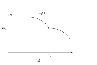
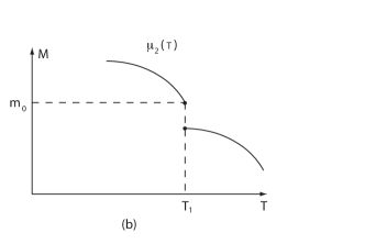
Figure 5.1. (a) The graph of function $\mu_{1}(T)$; (b) the graph of function $\mu_{2}(T)$.

On the other hand, by direct computation, the free energies of $M^{+}$ and $M^{-}$ are shown to be given by

$$G(M^{+})=\left\{\begin{aligned} &G(m_{0})&&\text{ if }T\geq T_{1},\\ &G(m_{0})+\frac{1}{4}(M^{+}_{1})^{2}(a_{2}M^{+}_{1}-\beta_{1})&&\text{ if }T<T_{1},\end{aligned}\right.$$

$$G(M^{-})=G(m_{0})+\frac{1}{4}(M^{-}_{1})^{2}(a_{2}M^{-}_{1}-\beta_{1}),$$

where $m_{0}$ is the magnetization induced by $H=(h,0,0)$ satisfying (5.3), and $\beta_{1}(T_{1})=0$. It is clear that

(5.4) $$G(M^{+})>G(M^{-})\ \ \ \ \text{near}\ T=T_{1}.$$

Hence, it follows from (5.4) that the magnetization behavior described by $\mu_{2}(T)$ is prohibited in real world because the free energy can not abruptly increase (or decrease) in a temperature decreasing (or increasing) process. Thus, by Theorem 4.1 and (5.4) we can derive the following physical conclusion:

Physical Conclusion 5.1.When an external field $H$ is present, the magnetization $M_{H}(T)$ of an isotropic ferromagnetic system is continuous on the temperature $T$, and there is a $T_{1}(H)>T_{c}$ ($T_{c}$ the Curie temperature) with $T_{1}(H)\rightarrow T_{c}$ as $H\rightarrow 0$ such that $M_{H}(T)$ is not differentiable at $T=T_{1}$, whose derivative has a finite jump

$$M^{\prime}_{H}(T_{1}^{-})-M^{\prime}_{H}(T_{1}^{+})=a>0\ \ \ \ (a<\infty).$$

Moreover, the graph of $M_{H}(T)=\mu_{1}(T)$ as shown in Figure 5.1(a), and $M_{H}(T)\rightarrow M_{0}(T)$ as $H\rightarrow 0$ with

$$M_{0}(T)=\left\{\begin{aligned} &0&&\text{ if }T\geq T_{c},\\ &M_{s}(T)&&\text{ if }T<T_{c},\end{aligned}\right.$$

where $M_{s}(T)$ is the spontaneous magnetization (see Figure 3.3).

5.2. Asymmetry of fluctuations

The above discussions suggest that for ferromagnetic systems, there are two possible phase transition behaviors near a critical point, and theoretically each of them has some probability to take place, however only one of them can appear in reality. For the ferromagnetic systems we again see this situation. This phenomena is also observed in phase transitions for PVT systems [2].

One explanation of such phenomena is that the symmety of fluctuation near a critical point is not generally true in equilibrium phase transitions. To make the statement more clear, we first introduce some concepts.

Let $G(u,\lambda)$ be free energy of a thermodynamic system, $u=(u_{1},\cdots,u_{n})$ be the order parameter, and $\lambda=(\lambda_{1},\cdots,\lambda_{m})$ the control parameter $(n,m\geq 1)$. Assume that $u$ is defined in the function space $L^{2}(\Omega,\mathbb{R}^{n})$ and $\lambda\in\mathbb{R}^{m}$. Then the space

$$X=\{(u,\lambda)|\ u\in L^{2}(\Omega,\mathbb{R}^{n}),\lambda\in\mathbb{R}^{m}\}$$

is called the state space of the system.

Let $(u_{0},\lambda_{0})\in X$ be a stable equilibrium state of the system; namely $(u_{0},\lambda_{0})$ is a locally minimal state of $G(u,\lambda)$. We say that the system has a fluctuation at $(u_{0},\lambda_{0})$ if it deviates randomly from $(u_{0},\lambda_{0})$ to $(\widetilde{u},\widetilde{\lambda})$ with

$$\|\widetilde{u}-u_{0}\|+|\widetilde{\lambda}-\lambda_{0}|>0.$$

In this case, $(\widetilde{u},\widetilde{\lambda})$ is called a state of fluctuation.

The so called symmetry of fluctuation means that for given $r>0$, all states $(\widetilde{u},\widetilde{\lambda})$ of fluctuation satisfying

$$\|\widetilde{u}-u_{0}\|+|\widetilde{\lambda}-\lambda_{0}|=r,\ \ \ \ (\widetilde{u},\widetilde{\lambda})\in X,$$

have the same probability to appear in real world. Otherwise, we say that the fluctuation is asymmetric.

The observations in both the PVT systems and the ferromagnetic systems strongly suggest the following physical conjecture, regarding to the uniqueness of transition behaviors.

Physical Conjecture (Asymmetry of Fluctuations). The symmetry of fluctuations for general thermodynamic systems may not be universally true. In other words, in some systems with multi-equilibrium states, the fluctuations near a critical point occur only in one basin of attraction of some equilibrium states, which are the ones that can be physically observed.

Appendix A Recapitulation of the Dynamic Transition Theory

In this appendix we recall some basic elements of the dynamic transition theory developed by the authors [1, 3], which are used to carry out the dynamic transition analysis for the ferromagnetism systems in this article.

Let $X$ and $X_{1}$ be two Banach spaces, $X_{1}\subset X$ a compact and dense inclusion. In this chapter, we always consider the following nonlinear evolution equations

(A.1) $$\left.\begin{aligned} &\frac{du}{dt}=L_{\lambda}u+G(u,\lambda),\\ &u(0)=\varphi,\end{aligned}\right.$$

where $u:[0,\infty)\rightarrow X$ is unknown function, and $\lambda\in\mathbb{R}^{1}$ is the system parameter.

Assume that $L_{\lambda}:X_{1}\rightarrow X$ is a parameterized linear completely continuous field depending contiguously on $\lambda\in\mathbb{R}^{1}$, which satisfies

(A.2) $$\left.\begin{aligned} &L_{\lambda}=-A+B_{\lambda}&&\text{a sectorial operator},\\ &A:X_{1}\rightarrow X&&\text{a linear homeomorphism},\\ &B_{\lambda}:X_{1}\rightarrow X&&\text{a linear compact operator}.\end{aligned}\right.$$

In this case, we can define the fractional order spaces $X_{\sigma}$ for $\sigma\in\mathbb{R}^{1}$. Then we also assume that $G(\cdot,\lambda):X_{\alpha}\rightarrow X$ is $C^{r}(r\geq 1)$ bounded mapping for some $0\leq\alpha<1$, depending continuously on $\lambda\in\mathbb{R}^{1}$, and

(A.3) $$G(u,\lambda)=o(\|u\|_{X_{\alpha}}),\ \ \ \ \forall\lambda\in\mathbb{R}^{1}.$$

Hereafter we always assume the conditions (A.2) and (A.3), which represent that the system (A.1) has a dissipative structure.

In the following we introduce the definition of transitions for (A.1).

Definition A.1.

We say that the system (A.1) has a transition of equilibrium from $(u,\lambda)=(0,\lambda_{0})$ on $\lambda>\lambda_{0}$ (or $\lambda<\lambda_{0})$ if the following two conditions are satisfied:

• when $\lambda<\lambda_{0}$ (or $\lambda>\lambda_{0}),u=0$ is locally asymptotically stable for (A.1); and

• when $\lambda>\lambda_{0}$ (or $\lambda<\lambda_{0})$, there exists a neighborhood $U\subset X$ of $u=0$ independent of $\lambda$, such that for any $\varphi\in U\setminus\Gamma_{\lambda}$ the solution $u_{\lambda}(t,\varphi)$ of (A.1) satisfies that

  $$\left.\begin{aligned} &\limsup_{t\rightarrow\infty}\|u_{\lambda}(t,\varphi)\|_{X}\geq\delta(\lambda)>0,\\ &\lim_{\lambda\rightarrow\lambda_{0}}\delta(\lambda)\geq 0,\end{aligned}\right.$$

  where $\Gamma_{\lambda}$ is the stable manifold of $u=0$, with codim $\Gamma_{\lambda}\geq 1$ in $X$ for $\lambda>\lambda_{0}$ (or $\lambda<\lambda_{0})$.

Obviously, the attractor bifurcation of (A.1) is a type of transition. However, bifurcation and transition are two different, but related concepts. Definition A.1 defines the transition of (A.1) from a stable equilibrium point to other states (not necessary equilibrium state). In general, we can define transitions from one attractor to another as follows.

Definition A.2.

Let $\Sigma_{\lambda}\subset X$ be an invariant set of (A.1). We say that (A.1) has a transition of states from $(\Sigma_{\lambda_{0}},\lambda_{0})$ on $\lambda>\lambda_{0}$ (or $\lambda<\lambda_{0})$ if the following conditions are satisfied:

• when $\lambda<\lambda_{0}$ (or $\lambda>\lambda_{0}),\Sigma_{\lambda}$ is a local minimal attractor, and

• when $\lambda>\lambda_{0}$ (or $\lambda<\lambda_{0})$, there exists a neighborhood $U\subset X$ of $\Sigma_{\lambda}$ independent of $\lambda$ such that for any $\varphi\in U\setminus(\Gamma_{\lambda}\cup\Sigma_{\lambda})$, the solution $u(t,\varphi)$ of (A.1) satisfies that

  $$\left.\begin{aligned} &\limsup_{t\rightarrow\infty}\text{\rm dist}(u(t,\varphi),\Sigma_{\lambda})\geq\delta(\lambda)>0,\\ &\lim\limits_{\lambda\rightarrow\lambda_{0}}\delta(\lambda)=\delta\geq 0,\end{aligned}\right.$$

  where $\Gamma_{\lambda}$ is the stable manifolds of $\Sigma_{\lambda}$ with codim $\Gamma_{\lambda}\geq 1$.

Let the eigenvalues (counting multiplicity) of $L_{\lambda}$ be given by

$$\{\beta_{j}(\lambda)\in\mathbb{C}\ \ |\ \ j=1,2,\cdots\}$$

Assume that

(A.4) $$\text{Re}\ \beta_{i}(\lambda)\left\{\begin{aligned} &<0&&\text{ if }\lambda<\lambda_{0},\\ &=0&&\text{ if }\lambda=\lambda_{0},\\ &>0&&\text{ if }\lambda>\lambda_{0},\end{aligned}\right. \forall 1\leq i\leq m,$$

(A.5) $$\text{Re}\ \beta_{j}(\lambda_{0})<0 \forall j\geq m+1.$$

The following theorem is a basic principle of transitions from equilibrium states, which provides sufficient conditions and a basic classification for transitions of nonlinear dissipative systems. This theorem is a direct consequence of the center manifold theorems and the stable manifold theorems; we omit the proof.

Theorem A.1.

Let the conditions (A.4) and (A.5) hold true. Then, the system (A.1) must have a transition from $(u,\lambda)=(0,\lambda_{0})$, and there is a neighborhood $U\subset X$ of $u=0$ such that the transition is one of the following three types:

• Continuous Transition: there exists an open and dense set $\widetilde{U}_{\lambda}\subset U$ such that for any $\varphi\in\widetilde{U}_{\lambda}$, the solution $u_{\lambda}(t,\varphi)$ of (A.1) satisfies

  $$\lim\limits_{\lambda\rightarrow\lambda_{0}}\limsup_{t\rightarrow\infty}\|u_{\lambda}(t,\varphi)\|_{X}=0.$$

  In particular, the attractor bifurcation of (A.1) at $(0,\lambda_{0})$ is a continuous transition.

• Jump Transition: for any $\lambda_{0}<\lambda<\lambda_{0}+\varepsilon$ with some $\varepsilon>0$, there is an open and dense set $U_{\lambda}\subset U$ such that for any $\varphi\in U_{\lambda}$,

  $$\limsup_{t\rightarrow\infty}\|u_{\lambda}(t,\varphi)\|_{X}\geq\delta>0,$$

  where $\delta>0$ is independent of $\lambda$. This type of transition is also called the discontinuous transition.

• Mixed Transition: for any $\lambda_{0}<\lambda<\lambda_{0}+\varepsilon$ with some $\varepsilon>0$, $U$ can be decomposed into two open sets $U^{\lambda}_{1}$ and $U^{\lambda}_{2}$ ($U^{\lambda}_{i}$ not necessarily connected):

  $$\bar{U}=\bar{U}^{\lambda}_{1}+\bar{U}^{\lambda}_{2},\ \ \ \ U^{\lambda}_{1}\cap U^{\lambda}_{2}=\emptyset,$$

  such that

  $$\lim\limits_{\lambda\rightarrow\lambda_{0}}\limsup_{t\rightarrow\infty}\|u(t,\varphi)\|_{X}=0 \forall\varphi\in U^{\lambda}_{1},$$

  $$\limsup_{t\rightarrow\infty}\|u(t,\varphi)\|_{X}\geq\delta>0 \forall\varphi\in U^{\lambda}_{2}.$$

An important aspect of the transition theory is to determine which of the three types of transitions given by Theorem A.1 occurs in a specific problem. We refer the interested readers to [3, 1] for more discussions. Instead, here we consider the transition of (A.1) from a simple critical eigenvalue. Let the eigenvalues $\beta_{j}(\lambda)$ of $L_{\lambda}$ satisfy

(A.6) $$\left.\begin{aligned} &\beta_{1}(\lambda)\left\{\begin{aligned} &<0&&\text{ if }\lambda<\lambda_{0},\\ &=0&&\text{ if }\lambda=\lambda_{0},\\ &>0&&\text{ if }\lambda>\lambda_{0},\end{aligned}\right.\\ &\text{Re}\beta_{j}(\lambda_{0})<0&&\forall j\geq 2,\end{aligned}\right.$$

where $\beta_{1}(\lambda)$ is a real eigenvalue.

Let $e_{1}(\lambda)$ and $e^{*}_{1}(\lambda)$ be the eigenvectors of $L_{\lambda}$ and $L^{*}_{\lambda}$ respectively corresponding to $\beta_{1}(\lambda)$ with

$$L_{\lambda_{0}}e_{1}=0,\ \ \ \ L^{*}_{\lambda_{0}}e^{*}_{1}=0,\ \ \ \ <e_{1},e^{*}_{1}>=1.$$

Let $\Phi(x,\lambda)$ be the center manifold function of (A.1) near $\lambda=\lambda_{0}$. We assume that

(A.7) $$<G(xe_{1}+\Phi(x,\lambda_{0}),\lambda_{0}),e^{*}_{1}>=\alpha x^{k}+o(|x|^{k}),$$

where $k\geq 2$ an integer and $\alpha\neq 0$ a real number.

We have the following transition theorems.

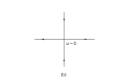
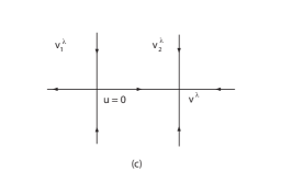
Figure A.1. Topological structure of the mixing transition of (A.1) when $k$=even and $\alpha\neq 0$: (a) $\lambda<\lambda_{0}$; (b) $\lambda=\lambda_{0}$; (c) $\lambda>\lambda_{0}$. Here $U^{\lambda}_{1}$ is the unstable domain, and $U^{\lambda}_{2}$ the stable domain.

Theorem A.2.

Under the conditions (A.6) and (A.7), if $k$=even and $\alpha\neq 0$, then we have the following assertions:

1. (A.1) has a mixed transition from $(0,\lambda_{0})$. More precisely, there exists a neighborhood $U\subset X$ of $u=0$ such that $U$ is separated into two disjoint open sets $U^{\lambda}_{1}$ and $U^{\lambda}_{2}$ by the stable manifold $\Gamma_{\lambda}$ of $u=0$ satisfying the following properties:

   1. $U=U^{\lambda}_{1}+U^{\lambda}_{2}+\Gamma_{\lambda}$,

   2. the transition in $U^{\lambda}_{1}$ is jump, and

   3. the transition in $U^{\lambda}_{2}$ is continuous. The local transition structure is as shown in Figure A.1.

2. (A.1) bifurcates in $U^{\lambda}_{2}$ to a unique singular point $v^{\lambda}$ on $\lambda>\lambda_{0}$, which is an attractor such that for any $\varphi\in U^{\lambda}_{2}$,

   $$\lim\limits_{t\rightarrow\infty}\|u(t,\varphi)-v^{\lambda}\|_{X}=0,$$

   where $u(t,\varphi)$ is the solution of (A.1).

3. (A.1) bifurcates on $\lambda<\lambda_{0}$ to a unique saddle point $v^{\lambda}$ with the Morse index one.

4. The bifurcated singular point $v^{\lambda}$ can be expressed as

   $$v^{\lambda}=-(\beta_{1}(\lambda)/\alpha)^{{1}/{(k-1)}}e_{1}+o(|\beta_{1}|^{{1}/{(k-1)}}).$$

References

- [1] T. Ma and S. Wang, Bifurcation theory and applications, vol. 53 of World Scientific Series on Nonlinear Science. Series A: Monographs and Treatises, World Scientific Publishing Co. Pte. Ltd., Hackensack, NJ, 2005.
- [2] , Dynamic phase transitions in pvt systems, submitted, (2007).
- [3] , Stability and Bifurcation of Nonlinear Evolution Equations, Science Press, 2007.
- [4] A. Onuki, Phase transition dynamics, Cambridge University Press, 2007.
- [5] L. E. Reichl, A modern course in statistical physics, A Wiley-Interscience Publication, John Wiley & Sons Inc., New York, second ed., 1998.