Critical behavior of magnetic thin films as a function of thickness

Abstract

We study the critical behavior of magnetic thin films as a function of the film thickness. We use the ferromagnetic Ising model with the high-resolution multiple histogram Monte Carlo (MC) simulation. We show that though the 2D behavior remains dominant at small thicknesses, there is a systematic continuous deviation of the critical exponents from their 2D values. We observe that in the same range of varying thickness the deviation of the exponent $\nu$ is rather small, while exponent $\beta$ suffers a larger deviation. We explain these deviations using the concept of ”effective” exponents suggested by Capehart and Fisher in a finite-size analysis. The shift of the critical temperature with the film thickness obtained here by MC simulation is in an excellent agreement with their prediction.

I Introduction

During the last 30 years. physics of surfaces and objects of nanometric size have attracted an immense interest. This is due to important applications in industry.zangwill ; bland-heinrich An example is the so-called giant magneto-resistance (GMR) used in data storage devices, magnetic sensors, … Baibich ; Grunberg ; Fert ; review In parallel to these experimental developments, much theoretical effortBinder-surf ; Diehl has also been devoted to the search of physical mechanisms lying behind new properties found in nanoscale objects such as ultrathin films, ultrafine particles, quantum dots, spintronic devices etc. This effort aimed not only at providing explanations for experimental observations but also at predicting new effects for future experiments.

The physics of two-dimensional (2D) systems is very exciting. Some of those 2D systems can be exactly solved: one famous example is the Ising model on the square lattice which has been solved by Onsager.Onsager This model shows a phase transition at a finite temperature $T_{c}$ given by $\sinh^{2}(2J/k_{B}T_{c})=1$ where $J$ is the nearest-neighbor (NN) interaction. Another interesting result is the absence of long-range ordering at finite temperatures for the continuous spin models (XY and Heisenberg models) in 2D.Mermin In general, three-dimensional (3D) systems for any spin models cannot be unfortunately solved. However, several methods in the theory of phase transitions and critical phenomena can be used to calculate the critical behaviors of these systems.Zinn

This paper deals with systems between 2D and 3D. Many theoretical studies have been devoted to thermodynamic properties of thin films, magnetic multilayers,… Binder-surf ; Diehl ; ngo2004trilayer ; Diep1989sl ; diep91-af-films In spite of this, several points are still not yet understood. It is known a long time ago that the presence of a surface in magnetic materials can give rise to surface spin-waves which are localized in the vicinity of the surface.diep79 These localized modes may be acoustic with a low-lying energy or optical with a high energy, in the spin-wave spectrum. Low-lying energy modes contribute to reduce in general surface magnetization at finite temperatures. One of the consequences is the surface disordering which may occur at a temperature lower than that for interior magnetization.diep81 The existence of low-lying surface modes depends on the lattice structure, the surface orientation, the surface parameters, surface conditions (impurities, roughness, …) etc. There are two interesting cases: in the first case a surface transition occurs at a temperature distinct from that of the interior spins and in the second case the surface transition coincides with the interior one, i. e. existence of a single transition. Theory of critical phenomena at surfacesBinder-surf ; Diehl and Monte Carlo (MC) simulationsLandau1 ; Landau2 of critical behavior of the surface-layer magnetization at the extraordinary transition in the three-dimensional Ising model have been carried out. These works suggested several scenarios in which the nature of the surface transition and the transition in thin films depends on many factors in particular on the symmetry of the Hamiltonian and on surface parameters.

We confine ourselves here in the case of a simple cubic film with Ising model. For our purpose, we suppose all interactions are the same everywhere even at the surface. This case is the simplest case where there is no surface-localized spin-wave modes and there is only a single phase transition at a temperature for the whole system (no separate surface phase transition).diep79 ; diep81 Other complicated cases will be left for future investigations. However, some preliminary discussions on this point for complicated surfaces have been reported in some of our previous papers.ngo2007 ; ngo2007fcc In the case of a simple cubic film with Ising model, Capehart and Fisher have studied the critical behavior of the susceptibility using a finite-size scaling analysis.Fisher They showed that there is a crossover from 2D to 3D behavior as the film thickness increases. The so-called ”effective” exponent $\gamma$ has been shown to vary according to a scaling function depending both on the film thickness and the distance to the transition temperature. As will be seen below the scaling suggested by Capehart and Fisher is in agreement with what we find here using extensive MC simulation.

The aim of this paper is to investigate the effect of the thickness on the critical exponents of the film. To carry out these purposes, we shall use MC simulations with highly accurate multiple histogram technique.Ferrenberg1 ; Ferrenberg2 ; Bunker

The paper is organized as follows. Section II is devoted to a description of the model and method. Results are shown and discussed in section III. Concluding remarks are given in section IV.

II Model and Method

II.1 Model

Let us consider the Ising spin model on a film made from a ferromagnetic simple cubic lattice. The size of the film is $L\times L\times N_{z}$. We apply the periodic boundary conditions (PBC) in the $xy$ planes to simulate an infinite $xy$ dimension. The $z$ direction is limited by the film thickness $N_{z}$. If $N_{z}=1$ then one has a 2D square lattice.

The Hamiltonian is given by

$$\mathcal{H}=-\sum_{\left<i,j\right>}J_{i,j}\sigma_{i}\cdot\sigma_{j}$$ (1)

where $\sigma_{i}$ is the Ising spin of magnitude 1 occupying the lattice site $i$, $\sum_{\left<i,j\right>}$ indicates the sum over the NN spin pairs $\sigma_{i}$ and $\sigma_{j}$.

In the following, the interaction between two NN surface spins is denoted by $J_{s}$, while all other interactions are supposed to be ferromagnetic and all equal to $J=1$ for simplicity. Let us note in passing that in the semi-infinite crystal the surface phase transition occurs at the bulk transition temperature when $J_{s}\simeq 1.52J$. This point is called ”extraordinary phase transition” which is characterized by some particular critical exponents.Landau1 ; Landau2 In the case of thin films, i. e. $N_{z}$ is finite, it has been theoretically shown that when $J_{s}=1$ the bulk behavior is observed when the thickness becomes larger than a few dozens of atomic layers:diep79 surface effects are insignificant on thermodynamic properties such as the value of the critical temperature, the mean value of magnetization at a given $T$, … When $J_{s}$ is smaller than $J$, surface magnetization is destroyed at a temperature lower than that for bulk spins.diep81 The criticality of a film with uniform interaction, i.e. $J_{s}=J$, has been studied by Capehart and Fisher as a function of the film thickness using a scaling analysisFisher and by MC simulations.Schilbe ; Caselle The results by Capehart and Fisher indicated that as long as the film thickness is finite the phase transition is strictly that of the 2D Ising universality class. However, they showed that at a temperature away from the transition temperature $T_{c}(N_{z})$, the system can behave as a 3D one when the spin-spin correlation length $\xi(T)$ is much smaller than the film thickness, i. e. $\xi(T)/N_{z}\ll 1$. As $T$ gets very close to $T_{c}(N_{z})$, $\xi(T)/N_{z}\rightarrow 1$, the system undergoes a crossover to 2D criticality. We will return to this work for comparison with our results shown below.

II.2 Multiple histogram technique

The multiple histogram technique is known to reproduce with very high accuracy the critical exponents of second order phase transitions.Ferrenberg1 ; Ferrenberg2 ; Bunker

The overall probability distributionFerrenberg2 at temperature $T$ obtained from $n$ independent simulations, each with $N_{j}$ configurations, is given by

$$P(E,T)=\frac{\sum_{i=1}^{n}H_{i}(E)\exp[E/k_{B}T]}{\sum_{j=1}^{n}N_{j}\exp[E/k_{B}T_{j}-f_{j}]},$$ (2)

where

$$\exp[f_{i}]=\sum_{E}P(E,T_{i}).$$ (3)

The thermal average of a physical quantity $A$ is then calculated by

$$\langle A(T)\rangle=\sum_{E}A\,P(E,T)/z(T),$$ (4)

in which

$$z(T)=\sum_{E}P(E,T).$$ (5)

Thermal averages of physical quantities are thus calculated as continuous functions of $T$, now the results should be valid over a much wider range of temperature than for any single histogram.

In MC simulations, one calculates the averaged order parameter $\langle M\rangle$ ($M$: magnetization of the system), averaged total energy $\langle E\rangle$, specific heat $C_{v}$, susceptibility $\chi$, first order cumulant of the energy $C_{U}$, and $n^{th}$ order cumulant of the order parameter $V_{n}$ for $n=1$ and 2. These quantities are defined as

$$\langle E\rangle = \langle\cal{H}\rangle,$$ (6)

$$C_{v} = \frac{1}{k_{B}T^{2}}\left(\langle E^{2}\rangle-\langle E\rangle^{2}\right),$$ (7)

$$\chi = \frac{1}{k_{B}T}\left(\langle M^{2}\rangle-\langle M\rangle^{2}\right),$$ (8)

$$C_{U} = 1-\frac{\langle E^{4}\rangle}{3\langle E^{2}\rangle^{2}},$$ (9)

$$V_{n} = \frac{\partial\ln{M^{n}}}{\partial(1/k_{B}T)}=\langle E\rangle-\frac{\langle M^{n}E\rangle}{\langle M^{n}\rangle}.$$ (10)

Let us discuss the case where all dimensions can go to infinity. For example, consider a system of size $L^{d}$ where $d$ is the space dimension. For a finite $L$, the pseudo ”transition” temperatures can be identified by the maxima of $C_{v}$ and $\chi$, …. These maxima do not in general take place at the same temperature. Only at infinite $L$ that the pseudo ”transition” temperatures of these respective quantities coincide at the real transition temperature $T_{c}(\infty)$. So when we work at the maxima of $V_{n}$, $C_{v}$ and $\chi$, we are in fact working at temperatures away from $T_{c}(\infty)$. Let us define the reduced temperature which measures the ”distance” from $T_{c}(\infty)$ by

$$t=\frac{T-T_{c}(\infty)}{T_{c}(\infty)}$$ (11)

This distance tends to zero when all dimensions go to infinity. For large values of $L$, the following scaling relations are expected (see details in Ref. Bunker, ):

$$V_{1}^{\max}\propto L^{1/\nu},\hskip 28.45274ptV_{2}^{\max}\propto L^{1/\nu},$$ (12)

$$C_{v}^{\max}=C_{0}+C_{1}L^{\alpha/\nu}$$ (13)

and

$$\chi^{\max}\propto L^{\gamma/\nu}$$ (14)

at their respective ’transition’ temperatures $T_{c}(L)$, and

$$C_{U}=C_{U}[T_{c}(\infty)]+AL^{-\alpha/\nu},$$ (15)

$$M_{T_{c}(\infty)}\propto L^{-\beta/\nu}$$ (16)

and

$$T_{c}(L)=T_{c}(\infty)+C_{A}L^{-1/\nu},$$ (17)

where $A$, $C_{0}$, $C_{1}$ and $C_{A}$ are constants. We estimate $\nu$ independently from $V_{1}^{\max}$ and $V_{2}^{\max}$. With this value we calculate $\gamma$ from $\chi^{\max}$ and $\alpha$ from $C_{v}^{\max}$. Note that we can estimate $T_{c}(\infty)$ using the last expression. Then, using $T_{c}(\infty)$, we can calculate $\beta$ from $M_{T_{c}(\infty)}$. The Rushbrooke scaling law $\alpha+2\beta+\gamma=2$ is then in principle verified.

Let us emphasize that the expressions Eqs. (12)-(17) are valid for large $L$. To be sure that $L$ are large enough, one has to allow for corrections to scaling of the form, for example,

$$\chi^{\max} = B_{1}L^{\gamma/\nu}(1+B_{2}L^{-\omega})$$ (18)

$$V_{n}^{\max} = D_{1}L^{1/\nu}(1+D_{2}L^{-\omega})$$ (19)

where $B_{1}$, $B_{2}$, $D_{1}$ and $D_{2}$ are constants and $\omega$ is a correction exponent.Ferrenberg3 Similar forms exist also for the other exponents. Usually, these corrections are extremely small if $L$ is large enough as is the case with today’s large-memory computers. So, in general they do not therefore alter the results using Eqs. (12)-(17).

II.3 The case of films with finite thickness

In the case of a thin film of size $L\times L\times N_{z}$, Capehart and FisherFisher have showed that as long as the film thickness $N_{z}$ is not allowed to go to infinity, there is a 2D-3D crossover if one does not work at the real transition temperature $T_{c}(L=\infty,N_{z})$. Following Capehart and Fisher, let us define

$$\dot{t} = \frac{T-T_{c}(L=\infty,N_{z})}{T_{c}(3D)}$$ (20)

$$x = N_{z}^{1/\nu_{3D}}\dot{t}$$ (21)

where $\nu_{3D}$ is the 3D $\nu$ exponent and $T_{c}(3D)$ the 3D critical temperature. When $x$ is larger than a value $x_{0}$, i. e. at a temperature away from $T_{c}(L=\infty,N_{z})$, the system behaves as a 3D one. While when $x<x_{0}$, it should behave as a 2D one. This crossover was argued from a comparison of the correlation length in the $z$ direction to the film thickness. As a consequence, if we work exactly at $T_{c}(L=\infty,N_{z})$ we should observe the 2D critical exponents for finite $N_{z}$. Otherwise, we should observe the so-called ”effective critical exponents” whose values are found between those of 2D and 3D cases. This point is fundamentally very important. There have been some attempts to verify it by MC simulations,Schilbe but these results were not convincing due to their poor MC quality. In the following we show with high-precision MC technique that the prediction of Capehart and Fisher is really verified.

III Results

The $xy$ linear sizes $L=20,24,30,...,80$ have been used in our simulations. For $N_{z}=3$, sizes up to 160 have been used to evaluate corrections to scaling.

In practice, we use first the standard MC simulations to localize for each size the transition temperatures $T^{E}_{0}(L)$ for specific heat and $T^{m}_{0}(L)$ for susceptibility. The equilibrating time is from 200000 to 400000 MC steps/spin and the averaging time is from 500000 to 1000000 MC steps/spin. Next, we make histograms at $8$ different temperatures $T_{j}(L)$ around the transition temperatures $T^{E,m}_{0}(L)$ with 2 millions MC steps/spin, after discarding 1 millions MC steps/spin for equilibrating. Finally, we make again histograms at $8$ different temperatures around the new transition temperatures $T^{E,m}_{0}(L)$ with $2\times 10^{6}$ and $4\times 10^{6}$ MC steps/spin for equilibrating and averaging time, respectively. Such an iteration procedure gives extremely good results for systems studied so far. Errors shown in the following have been estimated using statistical errors, which are very small thanks to our multiple histogram procedure, and fitting errors given by fitting software.

We note that only $\nu$ is directly calculated from MC data. Exponent $\gamma$ obtained from $\chi^{\max}$ and $\nu$ suffers little errors (systematic errors and errors from $\nu$). Other exponents are obtained by MC data and several-step fitting. For example, to obtain $\alpha$ we have to fit $C_{v}^{\max}$ of Eq. 13 by choosing $C_{0}$, $C_{1}$ and by using the value of $\nu$. So, in practice, in most cases, one calculates $\alpha$ or $\beta$ from MC data and uses the Rushbrooke scaling law to calculate the remaining exponent.

Now, similar to the discussion given in subsection II.2, if we work at a distance away from $T_{c}(L=\infty,N_{z})$ we should observe ”effective critical exponents”. This is the case because in the finite size analysis using the multiple histogram technique, we measure the maxima of $V_{n}$, $C_{V}$ and $\chi$ which occur at different temperatures for a finite $L$. These temperatures, though close to, are not $T_{c}(L=\infty,N_{z})$. To give a precision on this point, we show the values of these maxima and the corresponding temperatures for $N_{z}=7$ in Table 1. For the value of $T_{c}(L=\infty,N_{z}=7)$, see Table 2.

Table 1: Maxima and temperatures at the maxima of $V_{n}$ ($n=1,2$), $C_{v}$ and $\chi$ for various $L$ with $N_{z}=7$.

L	$C_{v}^{max}$	$\chi^{max}$	$V_{1}^{max}$	$V_{2}^{max}$	$Tc(C_{v}^{max})$	$T_{c}(\chi^{max})$	$T_{c}(V_{1}^{max})$	$T_{c}(V_{2}^{max})$
30	2.21115658	25.29532589	164.05948154	275.71581036	4.19027500	4.22755000	4.24277500	4.24900000
40	2.36517434	41.20958927	219.30094769	368.72462473	4.19305000	4.21895000	4.23025000	4.23500000
50	2.50496719	60.82008190	275.66203381	463.17327477	4.19275000	4.21340000	4.22210000	4.22600000
60	2.59177903	82.96529587	329.65536262	554.47606570	4.19270000	4.20940000	4.21710000	4.22045000
70	2.70129995	109.00528127	387.47245040	651.24905512	4.19250000	4.20640000	4.21260000	4.21530000
80	2.76931676	138.78113065	443.00488386	743.61068938	4.19220000	4.20410000	4.20965000	4.21205000

Given this fact, we emphasize that calculations using Eqs. (12)-(17) will give effective critical exponents except of course for the case $N_{z}=1$ where the results correspond to real critical exponents.

We show now the results obtained by MC simulations with the Hamiltonian (1). We have tested that all exponents do not change in the finite size scaling with $L\geq 30$. So most of results are shown for $L\geq 30$ except for $\nu$ where the lowest sizes $L=20,24$ can be used without modifying its value.

Let us show in Fig. 1 the layer magnetizations and their corresponding susceptibilities of the first three layers, in the case where $J_{s}=1$. It is interesting to note that the surface layer is smaller that the interior layers, as it has been shown theoretically by the Green’s function method a long time ago.diep79 ; diep81 The surface spins have smaller local field due to the lack of neighbors, so thermal fluctuations will reduce more easily the surface magnetization with respect to the interior ones. The susceptibilities have their peaks at the same temperature, indicating a single transition.

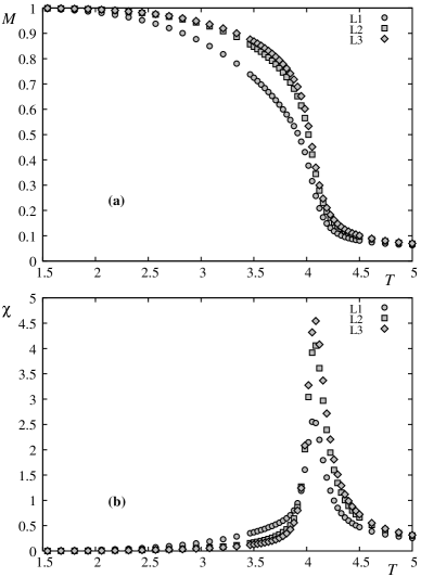
Figure 1: Layer magnetizations (a) and layer susceptibilities (b) versus $T$ with $N_{z}=5$ and $L=24$.

Figure 2 shows total magnetization of the film and the total susceptibility. This indicates clearly that there is only one peak as said above.

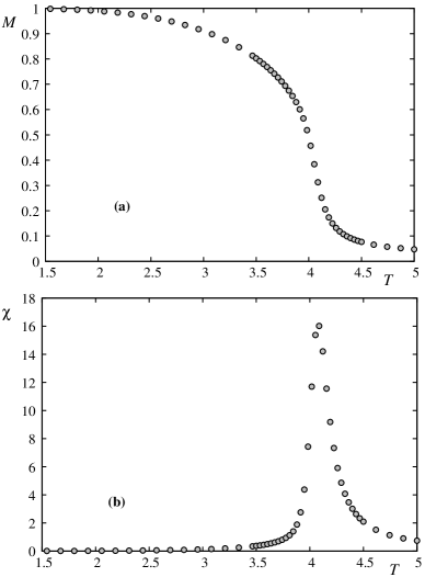
Figure 2: Total magnetization (a) and total susceptibility (b) versus $T$ with $N_{z}=5$ and $L=24$.

III.1 Finite size scaling

Let us show some results obtained from multiple histograms described above. Figure 3 shows the susceptibility and the first derivative $V_{1}$ versus $T$ around their maxima for several sizes.

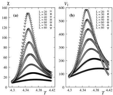
Figure 3: (a) Susceptibility and (b) $V_{1}$, as functions of $T$ for several $L$ with $N_{z}=11$, obtained by multiple histogram technique.

We show in Fig. 4 the maximum of the first derivative of $\ln M$ with respect to $\beta=(k_{B}T)^{-1}$ versus $L$ in the $\ln-\ln$ scale for several film thicknesses up to $N_{z}=13$. If we use Eq. (12) to fit these lines, i. e. without correction to scaling, we obtain $1/\nu$ from the slopes of the remarkably straight lines. These values are indicated on the figure. In order to see the deviation from the 2D exponent, we plot in Fig. 5 $\nu$ as a function of thickness $N_{z}$. We observe here a small but systematic deviation of $\nu$ from its 2D value ($\nu_{2D}=1)$ with increasing thickness. To show the precision of our method, we give here the results of $N_{z}=1$. For $N_{z}=1$, we have $1/\nu=1.0010\pm 0.0028$ which yields $\nu=0.9990\pm 0.0031$ and $\gamma/\nu=1.7537\pm 0.0034$ (see Figs. 6 and 7 below) yielding $\gamma=1.7520\pm 0.0062$. These results are in excellent agreement with the exact results $\nu_{2D}=1$ and $\gamma_{2D}=1.75$. The very high precision of our method is thus verified in the rather modest range of the system sizes $L=20-80$ used in the present work. Note that the result of Ref.Schilbe, gave $\nu=0.96\pm 0.05$ for $N_{z}=1$ which is very far from the exact value.

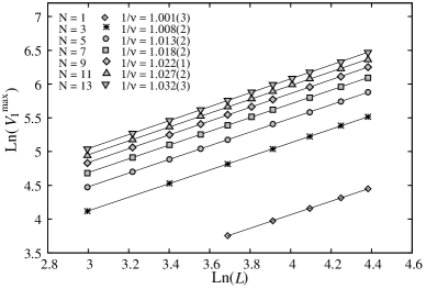
Figure 4: Maximum of the first derivative of $\ln M$ versus $L$ in the $\ln-\ln$ scale. The slopes are indicated on the figure.

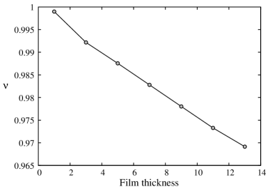
Figure 5: Effective exponent $\nu$ versus $N_{z}$.

The deviation of $\nu$ from the 2D value when $N_{z}$ increases is due, as discussed earlier, to the crossover to 3D ($\dot{t}$ is not zero). Other exponents will suffer the same deviations as seen below.

We show in Fig. 6 the maximum of the susceptibility versus $L$ in the $\ln-\ln$ scale for film thicknesses up to $N_{z}=13$. We have used only results of $L\geq 30$. Including $L=20$ and 24 will result, unlike the case of $\nu$, in a decrease of $\gamma$ of about one percent for $N_{z}\geq 7$. From the slopes of these straight lines, we obtain the values of effective $\gamma/\nu$. Using the values of $\nu$ obtained above, we deduce the values of $\gamma$ which are plotted in Fig. 7 as a function of thickness $N_{z}$. Unlike the case of $\nu$, we observe here a stronger deviation of $\gamma$ from its 2D value (1.75) with increasing thickness. This finding is somewhat interesting: the magnitude of the deviation from the 2D value may be different from one critical exponent to another: $\simeq 3\%$ for $\nu$ and $\simeq 8\%$ for $\gamma$ when $N_{z}$ goes from 1 to 13. We will see below that $\beta$ varies even more strongly.

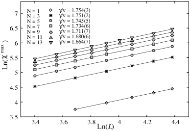
Figure 6: Maximum of susceptibility versus $L$ in the $\ln-\ln$ scale. The slopes are indicated on the figure.

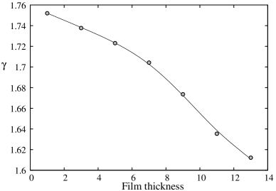
Figure 7: Effective exponent $\gamma$ versus $N_{z}$.

We show now in Fig. 8 the maximum of $C_{v}^{\max}$ versus $L$ for $N_{z}=1,3,5,...,13$. Note that for each $N_{z}$ we had to look for $C_{0}$, $C_{1}$ and $\alpha/\nu$ which give the best fit with data of $C_{v}^{\max}$. Due to the fact that there are several parameters which can induce a wrong combination of them, we impose that $\alpha$ should satisfy the condition $0\leq\alpha\leq 0.11$ where the lower limit of $\alpha$ corresponds to the value of 2D case and the upper limit to the 3D case. In doing so, we get very good results shown in Fig. 8. From these ratios of $\alpha/\nu$ we deduce $\alpha$ for each $N_{z}$. The values of $\alpha$ are shown in Table 2 for several $N_{z}$.

It is interesting to note that the effective exponents obtained above give rise to the effective dimension of thin film. This is conceptually not rigorous but this is what observed in experiments. Replacing the effective values of $\alpha$ obtained above in $d_{\mbox{eff}}=(2-\alpha)/\nu$ we obtain $d_{\mbox{eff}}$ shown in Fig. 9.

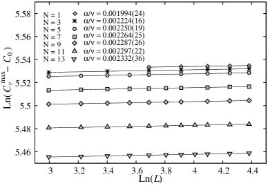
Figure 8: $\ln(C_{v}^{\max}-C_{0})$ versus $\ln L$ for $N_{z}=1,3,5,...,13$. The slope gives $\alpha/\nu$ (see Eq. 13) indicated on the figure.

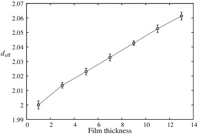
Figure 9: Effective dimension of thin film obtained by using effective exponents, as a function of thickness.

We note that $d_{\mbox{eff}}$ is very close to 2. It varies from 2 to $\simeq 2.061$ for $N_{z}$ going from 1 to 13. The 2D character is thus dominant even with larger $N_{z}$. This supports the idea that the finite correlation in the $z$ direction, though qualitatively causing a deviation, cannot strongly alter the 2D critical behavior. This point is interesting because, as said earlier, some thermodynamic properties may show already their 3D values at a thickness of about a few dozens of layers, but not the critical behavior. To show an example of this, let us plot in Fig. 10 the transition temperature at $L=\infty$ for several $N_{z}$, using Eq. 17 for each given $N_{z}$. As seen, $T_{c}(\infty)$ reaches already $\simeq 4.379$ at $N_{z}=13$ while its value at 3D is $4.51$.Ferrenberg3 ; Blote A rough extrapolation shows that the 3D values is attained for $N_{z}\simeq 25$ while the critical exponents at this thickness are far away from the 3D ones.

Let us show the prediction of Capehart and FisherFisher on the critical temperature as a function of $N_{z}$. Defining the critical-point shift as

$$\varepsilon(N_{z})=\left[T_{c}(L=\infty,N_{z})-T_{c}(3D)\right]/T_{c}(3D)$$ (22)

they showed that

$$\varepsilon(N_{z})\approx\frac{b}{N_{z}^{1/\nu}}[1+a/N_{z}]$$ (23)

where $\nu=0.6289$ (3D value). Using $T_{c}(3D)=4.51$, we fit the above formula with $T_{c}(L=\infty,N_{z})$ taken from Table 2, we obtain $a=-1.37572$ and $b=-1.92629$. The MC results and the fitted curve are shown in Fig. 10. Note that if we do not use the correction factor $[1+a/N_{z}]$, the fit is not good for small $N_{z}$. The prediction of Capehart and Fisher is thus very well verified.

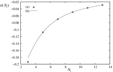
Figure 10: Critical temperature at infinite $L$ as a function of the film thickness. Points are MC results, continuous line is the prediction of Capehart and Fisher, Eq. (23). The agreement is excellent.

We give here the precise values of $T_{c}(L=\infty,N_{z})$ for each thickness. For $N_{z}=1$, we have $T_{c}(L=\infty,N_{z}=1)=2.2699\pm 0.0005$. Note that the exact value of $T_{c}(\infty)$ is 2.26919 by solving the equation $\sinh^{2}(2J/T_{c})=1$. Again here, the excellent agreement of our result shows the efficiency of the multiple histogram technique as applied in the present paper. The values of $T_{c}(L=\infty)$ for other $N_{z}$ are summarized in Table 2.

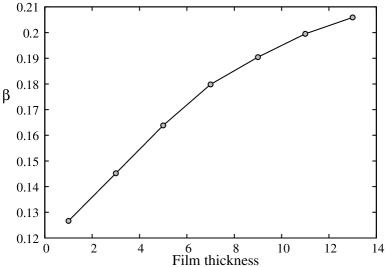
Figure 11: Effective exponent $\beta$, obtained by using Eq. 16, versus the film thickness.

Calculating now $M(L)$ at these values of $T_{c}(L=\infty,N_{z})$ and using Eq. 16, we obtain $\beta/\nu$ for each $N_{z}$. For $N_{z}=1$, we have $\beta/\nu=0.1268\pm 0.0022$ which yields $\beta=0.1266\pm 0.0049$ which is in excellent agreement with the exact result 0.125. Note that if we calculate $\beta$ from $\alpha+2\beta+\gamma=2$, then $\beta=(2-1.75198-0.00199)/2=0.12302\pm 0.0035$ which is in good agreement with the direct calculation within errors. We show in Fig. 11 the values of $\beta$ obtained by direct calculation using Eq. 16. Note that the deviation of $\beta$ from the 2D value when $N_{z}$ varies from 1 to 13 is due to the crossover effect discussed in subsection II.3. It represents about 60$\%$. Remember that the 3D value of $\beta$ is $0.3258\pm 0.0044$.Ferrenberg3

Finally, for convenience, let us summarize our results in Table 2 for $N_{z}=1,3,...,13$. Except for $N_{z}=1$, all other cases are effective exponents discussed above. Due to the smallness of $\alpha$, its value is shown with 5 decimals without rounding.

Table 2: Critical exponents, effective dimension and critical temperature at infinite $xy$ limit as obtained in this paper.

$N_{z}$	$\nu$	$\gamma$	$\alpha$	$\beta$	$d_{\mathrm{eff}}$	$T_{c}(L=\infty,N_{z})$
1	$0.9990\pm 0.0028$	$1.7520\pm 0.0062$	$0.00199\pm 0.00279$	$0.1266\pm 0.0049$	$2.0000\pm 0.0028$	$2.2699\pm 0.0005$
3	$0.9922\pm 0.0019$	$1.7377\pm 0.0035$	$0.00222\pm 0.00192$	$0.1452\pm 0.0040$	$2.0135\pm 0.0019$	$3.6365\pm 0.0024$
5	$0.9876\pm 0.0023$	$1.7230\pm 0.0069$	$0.00222\pm 0.00234$	$0.1639\pm 0.0051$	$2.0230\pm 0.0023$	$4.0234\pm 0.0028$
7	$0.9828\pm 0.0024$	$1.7042\pm 0.0087$	$0.00223\pm 0.00238$	$0.1798\pm 0.0069$	$2.0328\pm 0.0024$	$4.1939\pm 0.0032$
9	$0.9780\pm 0.0016$	$1.6736\pm 0.0084$	$0.00224\pm 0.00161$	$0.1904\pm 0.0071$	$2.0426\pm 0.0016$	$4.2859\pm 0.0022$
11	$0.9733\pm 0.0025$	$1.6354\pm 0.0083$	$0.00224\pm 0.00256$	$0.1995\pm 0.0088$	$2.0526\pm 0.0026$	$4.3418\pm 0.0032$
13	$0.9692\pm 0.0026$	$1.6122\pm 0.0102$	$0.00226\pm 0.00268$	$0.2059\pm 0.0092$	$2.0613\pm 0.0027$	$4.3792\pm 0.0034$

III.2 Larger sizes and correction to scaling

We consider here the effects of larger $L$ and of the correction to scaling. For the effect of larger $L$, we will extend our size up to $L=160$, for just the case $N_{z}=3$.

The results indicate that larger $L$ does not change the results shown above. Figure 12(a) displays the maximum of $V_{1}$ as a function of $L$ up to 160. Using Eq. (12), i. e. without correction to scaling, we obtain $1/\nu=1.009\pm 0.001$ which is to be compared to $1/\nu=1.008\pm 0.002$ using $L$ up to 80. The change is therefore insignificant because it is at the third decimal i. e. at the error level. The same is observed for $\gamma/\nu$ as shown in Fig. 12(b): $\gamma/\nu=1.752\pm 0.002$ using $L$ up to 160 instead of $\gamma/\nu=1.751\pm 0.002$ using $L$ up to 80.

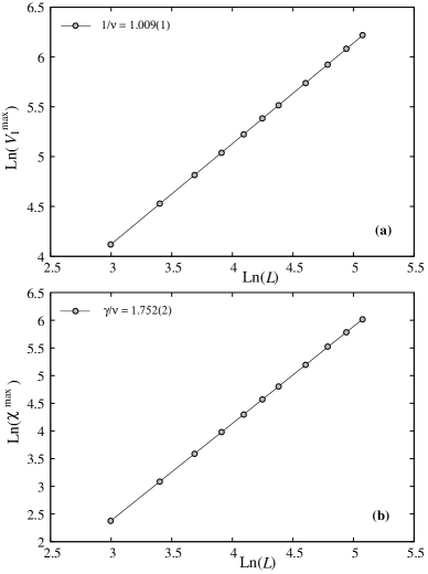
Figure 12: (a) $V_{1}^{max}$ and (b) $\chi^{max}$ vs $L$ up to 160 with $N_{z}=3$.

Now, let us allow for correction to scaling, i. e. we use Eq.(18) instead of Eq. (14) for fitting. We obtain the following values: $\gamma/\nu=1.751\pm 0.002$, $B_{1}=0.05676$, $B_{2}=1.57554$, $\omega=3.26618$ if we use $L$ = 70 to 160 (see Fig. 13). The value of $\gamma/\nu$ in the case of no scaling correction is $1.752\pm 0.002$. Therefore, we can conclude that this correction is insignificant. The large value of $\omega$ explains the smallness of the correction.

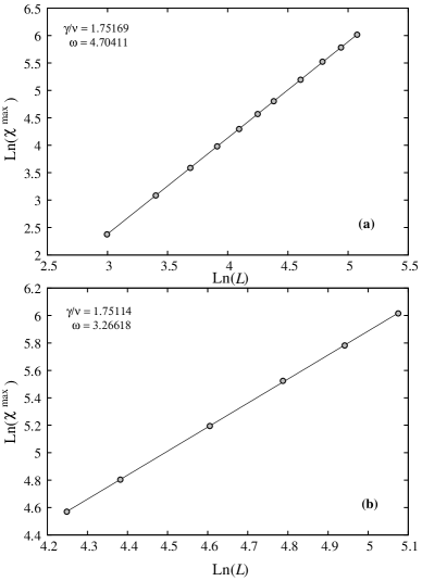
Figure 13: $\chi^{max}$ vs $L$ (a) from $20$ up to 160 (b) from $70$ up to 160, for $N_{z}=3$.

III.3 Role of boundary condition

To close this section, let us touch upon the question: does the absence of PBC in the $z$ direction cause the deviation of the critical exponents? The answer is no: we have calculated $\nu$ and $\gamma$ for $N_{z}=5$ in both cases, with and without PBC in the $z$ direction. The results show no significant difference between the two cases as seen in Figs. 14 and 15. We have found the same thing with $N_{z}=11$ shown in Figs. 16 and 17. So, we conclude that the fixed thickness will result in the deviation of the critical exponents, not from the absence of the PBC. This is somewhat surprising since we may think, incorrectly, that the PBC should mimic the infinite dimension so that we should obtain the 3D behavior when applying the PBC. As will be seen below, the 3D behavior is recovered only when the finite size scaling is applied in the $z$ direction at the same time in the $xy$ plane. To show this, we plot in Figs. 18 and 19 the results for the 3D case. Even with our modest sizes (up to $L=N_{z}=21$, since it is not our purpose to treat the 3D case here), we obtain $\nu=0.613\pm 0.005$ and $\gamma=1.250\pm 0.005$ very close to their 3D best known values $\nu_{3D}=0.6302\pm 0.0001$ from Ref. Blote, and $\nu_{3D}=0.6289\pm 0.0008$ and $\gamma_{3D}=1.2390\pm 0.0025$ obtained by using $24\leq L\leq 96$ given in Ref. Ferrenberg3, .

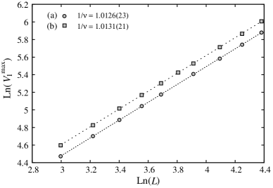
Figure 14: Maximum of the first derivative of $\ln M$ versus $L$ in the $\ln-\ln$ scale for $N_{z}=5$ (a) without PBC in $z$ direction (b) with PBC in $z$ direction. The slopes are indicated on the figure. See text for comments.

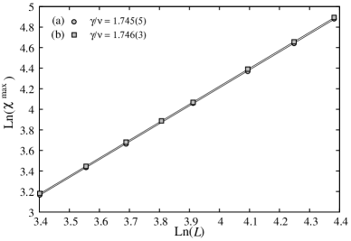
Figure 15: Maximum of susceptibility versus $L$ in the $\ln-\ln$ scale for $N_{z}=5$ (a) without PBC in $z$ direction (b) with PBC in $z$ direction. The points of these cases cannot be distinguished in the figure scale. The slopes are indicated on the figure. See text for comments.

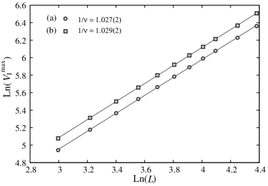
Figure 16: Maximum of the first derivative of $\ln M$ versus $L$ in the $\ln-\ln$ scale for $N_{z}=11$ (a) without PBC in $z$ direction (b) with PBC in $z$ direction. The slopes are indicated on the figure. See text for comments.

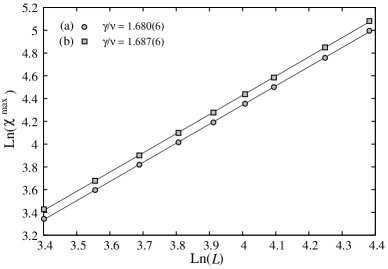
Figure 17: Maximum of susceptibility versus $L$ in the $\ln-\ln$ scale for $N_{z}=11$ (a) without PBC in $z$ direction (b) with PBC in $z$ direction. The slopes are indicated on the figure. See text for comments.

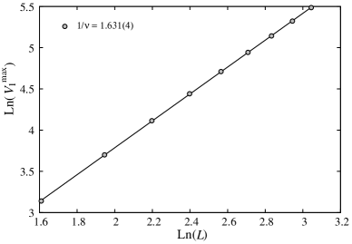
Figure 18: Maximum of the first derivative of $\ln M$ versus $L$ in the $\ln-\ln$ scale for 3D case.

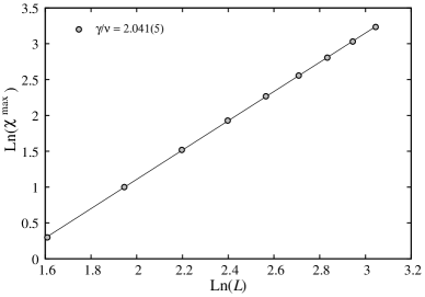
Figure 19: Maximum of susceptibility versus $L$ in the $\ln-\ln$ scale for 3D case.

IV Concluding remarks

We have considered a simple system, namely the Ising model on a simple cubic thin film, in order to clarify the point whether or not there is a continuous deviation of the 2D exponents with varying film thickness. From results obtained by the highly accurate multiple histogram technique shown above, we conclude that the critical exponents in thin films show a continuous deviation from their 2D values as soon as the thickness departs from 1. This deviation stems from a deep physical mechanism: Capehart and FisherFisher have argued that if one works exactly at the critical temperature $T_{c}(L=\infty,N_{z})$ then the critical exponents should be those of 2D universality class as long as the film thickness is finite. At $T_{c}(L=\infty,N_{z})$, the correlation in the $z$ direction $\xi$ remains finite while those in the $xy$ planes become infinite. Hence $\xi$ is irrelevant to the criticality. This yields therefore the 2D behavior. However, when the system is away from $T_{c}(L=\infty,N_{z})$, as is the case in numerical simulations using finite sizes, the system may have a 3D behavior as long as $\xi<<N_{z}$. This should yield a deviation of 2D critical exponents. The results we obtained in this paper verify this picture. In addition, the prediction of Capehart and Fisher for the shift of the critical temperature with the film thickness is in a perfect agreement with our simulations. Note furthermore that (i) the deviations of the exponents from their 2D values are very different in magnitude: while $\nu$ and $\alpha$ vary very little over the studied range of thickness, $\gamma$ and specially $\beta$ suffer stronger deviations, (ii) with a fixed thickness $N_{z}\neq 1$, the same ”effective” exponents are observed, within errors, in simulations with and without periodic boundary condition in the $z$ direction, (iii) to obtain the 3D behavior, the finite size scaling should be applied simultaneously in the three directions, i. e. all dimensions should be allowed to go to infinity. If we do not apply the scaling in the $z$ direction, we will not obtain 3D behavior even with a very large, but fixed, thickness and even with periodic boundary condition in the $z$ direction, (iv) with regard to the critical behavior, thin films behave as systems with effective critical exponents whose values are those between 2D and 3D.

To conclude, we hope that the numerical results shown in this paper will help experimentalists to interpret their data which are usually obtained at a finite distance from the critical point. It should be also desirable to study more cases to clarify the role of thickness on the behavior of very thin films, in particular the effect of the film thickness on the bulk first-order transition.

One of us (VTN) thanks the ”Asia Pacific Center for Theoretical Physics” (South Korea) for a financial post-doc support and hospitality during the period 2006-2007 where part of this work was carried out. The authors are grateful to Yann Costes of the University of Cergy-Pontoise for technical help in parallel computation.

References

- (1) A. Zangwill, Physics at Surfaces, Cambridge University Press (1988).
- (2) Ultrathin Magnetic Structures, vol. I and II, J.A.C. Bland and B. Heinrich (editors), Springer-Verlag (1994).
- (3) M. N. Baibich, J. M. Broto, A. Fert, F. Nguyen Van Dau, F. Petroff, P. Etienne, G. Creuzet, A. Friederich and J. Chazelas, Phys. Rev. Lett. 61, 2472 (1988).
- (4) P. Grunberg, R. Schreiber, Y. Pang, M. B. Brodsky and H. Sowers, Phys. Rev. Lett. 57, 2442 (1986); G. Binash, P. grunberg, F. Saurenbach and W. Zinn, Phys. Rev. B 39, 4828 (1989).
- (5) A. Barthélémy et al, J. Mag. Mag. Mater. 242-245, 68 (2002).
- (6) See review by E. Y. Tsymbal and D. G. Pettifor, Solid State Physics (Academic Press, San Diego), Vol. 56, pp. 113-237 (2001).
- (7) K. Binder, in Phase Transitions and Critical Phenomena, ed. by C. Domb, J.L. Lebowitz (Academic, London, 1983) vol. 8.
- (8) H.W. Diehl, in Phase Transitions and Critical Phenomena, ed. by C. Domb, J.L. Lebowitz (Academic, London, 1986) vol. 10, H.W. Diehl, Int. J. Mod. Phys. B 11, 3503 (1997).
- (9) L. Onsager, Phys. Rev. 65, 117 (1944).
- (10) N. D. Mermin and H. Wagner, Phys. Rev. Lett. 17, 1133 (1966).
- (11) J. Zinn-Justin, Quantum Field Theory and Critical Phenomena, Oxford University Press (4th edition - 2002).
- (12) H. T. Diep, Phys. Rev. B 40, 4818 (1989).
- (13) H. T. Diep, Phys. Rev. B 43, 8509 (1991).
- (14) See V. Thanh Ngo, H. Viet Nguyen, H. T. Diep and V. Lien Nguyen, Phys. Rev. B. 69, 134429 (2004) and references on magnetic multilayers cited therein.
- (15) H. T. Diep, J.C. S. Levy and O. Nagai, Phys. Stat. Solidi (b) 93, 351 (1979).
- (16) H. T. Diep, Phys. Stat. Solidi (b) , 103, 809 (1981).
- (17) D. P. Landau and K. Binder, Phys. Rev. B 41, 4786 (1990).
- (18) D. P. Landau and K. Binder, Phys. Rev. B 41, 4633 (1990).
- (19) See V. Thanh Ngo and H. T. Diep, Phys. Rev. B. 75, 035412 (2007) and references on surface effects cited therein.
- (20) See V. Thanh Ngo and H. T. Diep, cond-mat/arXiv:0705.1169.
- (21) T. W. Capehart and M. E. Fisher, Phys. Rev. B 13, 5021 (1976).
- (22) A. M. Ferrenberg and R. H. Swendsen, Phys. Rev. Let. 61, 2635 (1988).
- (23) A. M. Ferrenberg and R. H. Swendsen, Phys. Rev. Let. 63, 1195 (1989).
- (24) A. Bunker, B. D. Gaulin, and C. Kallin, Phys. Rev. B 48, 15861 (1993).
- (25) P. Schilbe, S. Siebentritt and K. H. Rieder, Phys. Lett. A 216, 20 (1996).
- (26) M. Caselle and M. Hasenbusch, Nucl.Phys. B 470, 435 (1996).
- (27) A. M. Ferrenberg and D. P. Landau, Phys. Rev. B 44, 5081 (1991).
- (28) Youjin Deng and Henk W. J. Blte, Phys. Rev. E 68, 036125 (2003).