Influence of photon-assisted tunneling on heat flow in a normal metal– superconductor tunnel junction

Abstract

We have investigated theoretically the influence of an AC drive on heat transport in a hybrid normal metal - superconductor tunnel junction in the photon-assisted tunneling regime. We find that the useful heat flux out from the normal metal is always reduced as compared to its magnitude under the static and quasi-static drive conditions. Our results are useful to predict the operative conditions of AC driven superconducting electron refrigerators.

I Introduction

Photon-assisted tunneling (PAT) has been discussed in literature for almost half a century by now dayem ; cook ; lax ; hamilton ; kommers ; prober ; vaknin ; yu ; wyder ; habbal ; mooij ; leone ; uzawa ; tien ; tucker ; tucker2 ; sweet ; zimmermann . This phenomenon arises when a relatively high frequency field is applied across a tunnel junction whose DC current-voltage characteristics are highly non-linear. The radiation field is, however, slow enough to guarantee adiabatic evolution of the energy levels of the electrons. A typical system to observe PAT is a SIS tunnel junction, with superconducting (S) leads and a tunnel barrier (I) in between. Even though the system as such is a Josephson junction for Cooper pairs, PAT deals with the influence of the radiation on quasiparticle tunneling. Our system of interest here is a NIS tunnel junction, where one of the conductors is a normal metal (N). Such junctions exhibit highly nonlinear current-voltage characteristics at low temperatures, and normally the current is due to quasiparticles only. NIS-junctions are known to have peculiar heat transport properties under the application of a DC bias voltage giazotto06 ; bardas ; leivo ; nahum ; clark ; clark2 ; savin ; leoni ; fs ; magbar ; fis , or (”quasi-static”) AC radiation of relatively low frequency in form of either periodic or stochastic drive pekola07a ; saira ; pekola07b . Specifically, it is possible to find operation regimes where the normal metal is refrigerated and the superconductor is overheated, and in some special situations the opposite can occur as well. The question remains whether and under what conditions the relatively high frequency radiation responsible for PAT would either enhance or suppress the thermal transport in the NIS-system. In this paper we show that the influence of PAT, as compared to static and quasi-static AC drive conditions, is to decrease the refrigeration of the normal conductor, and also to change, usually to increase, the magnitude of heat dissipation in the superconductor. Although these results are somewhat unfortunate for high-frequency applications of NIS-junctions, they are, however, useful in finding operating conditions, for instance, for AC driven electronic refrigerators pekola07a ; saira .

The paper is organized as follows. In Sec. II we describe the theoretical framework together with the discussion of the conditions of its validity. In particular, in Sec. II.1 we present our analytical results for the heat and charge currents. In Sec. III we show and discuss the results. Finally, our conclusion are drawn in Sec. IV.

II Model and formalism

The system under investigation consists of superconducting (S) and a normal (N) electrode tunnel-coupled through an insulating barrier (I) of large resistance $R_{t}$. An AC voltage bias $\varphi_{S}$, of frequency $\nu_{0}=\omega_{0}/2\pi$ and amplitude $V_{\text{ac}}$, is applied to the S electrode, while a static voltage $\varphi_{N}=U$ is applied to the N contact. The total voltage across the junction is $\varphi_{N}-\varphi_{S}=U-V_{ac}\cos\omega_{0}t$. One could, of course, consider both the AC and DC voltage to be applied to the normal lead, instead. However, we choose the setup as shown in Fig. 1 to directly demonstrate equivalence of the two connections when one of the leads is in the superconducting state.

Figure 1: The system under investigation is composed of a superconductor (S) tunnel-coupled to a normal metal (N) layer through an insulating barrier (I) of resistance $R_{t}$. The superconductor is AC voltage biased with $V_{\text{ac}}\cos(\omega_{0}t)$, while the N electrode is biased with a static voltage $U$. Both electrodes are assumed to be in thermal equilibrium.

In the tunnelling limit with large resistance $R_{t}$ the currents through the contact are small. If the AC frequency is small compared to the superconducting gap, $\omega_{0}\ll\Delta$, the deviation from equilibrium in each lead is negligible. In particular, the equilibrium is preserved with respect to the superconducting chemical potential $\mu_{S}$ in the S electrode (which has dimensions much bigger than the branch-imbalance relaxation length). This leads to the standard assumption tien ; tucker ; tucker2

$$\frac{\hbar}{2}\frac{\partial\chi}{\partial t}\equiv\mu_{S}=-e\varphi_{S}\ .$$ (1)

where $\chi$ is the order parameter phase.

In the case of equilibrium described by Eq. (1), the order parameter has the form

$$\Delta({\bf r},t)=\Delta_{0}({\bf r})\exp\left(\frac{2i}{\hbar}\int_{0}^{t}\mu_{s}\,dt^{\prime}\right)\ .$$ (2)

It is convenient to start with the Bogoliubov–de Gennes equation (BdGE) for the eigen-functions of the system,

$$i\hbar\frac{\partial u}{\partial t} = (\hat{H}_{0}+e\varphi_{S})u+\Delta v\ ,$$

$$i\hbar\frac{\partial v}{\partial t} = -(\hat{H}_{0}^{*}+e\varphi_{S})v+\Delta^{*}u\ ,$$

where $H_{0}$ is the normal-state Hamiltonian. Solutions to the BdGE have the form

$$u({\bf r},t) = u_{0}({\bf r})e^{-iEt/\hbar+(i/\hbar)\int^{t}\mu_{s}\,dt^{\prime}}\ ,$$ (3)

$$v({\bf r},t) = v_{0}({\bf r})e^{-iEt/\hbar-(i/\hbar)\int^{t}\mu_{s}\,dt^{\prime}}\ ,$$ (4)

where $u_{0}({\bf r})$ and $v_{0}({\bf r})$ satisfy the BdGE in the absence of the applied potential ($\varphi_{S}=0$)

$$Eu_{0} = \hat{H}_{0}u_{0}+\Delta({\bf r})v_{0}\ ,$$

$$Ev_{0} = -\hat{H}_{0}^{*}v_{0}+\Delta^{*}({\bf r})u_{0}\ .$$

Using the standard approach we define the retarded (R) and advanced (A) Green function, which can be written as a matrix in Nambu space:

$$\hat{G}^{R(A)}=\left(\begin{array}[]{cc}G^{R(A)}&F^{R(A)}\\ -F^{R(A)\dagger}&\bar{G}^{R(A)}\end{array}\right)\ ,$$

where $F^{R(A)}$ refer to the anomalous Gorkov function. Since these functions are statistical averages of the particle field operators which can be decomposed into the wave functions Eqs. (3) and (4), the retarded and advanced Green functions with help of Eqs. (3) and (4) take the form

$$G^{R(A)}(t_{1},t_{2}) = G^{R(A),0}(t_{1},t_{2})\,e^{i/\hbar(\int^{t_{1}}\mu_{s}\,dt^{\prime}-\int^{t_{2}}\mu_{s}\,dt^{\prime})}\ ,$$

$$\bar{G}^{R(A)}(t_{1},t_{2}) = \bar{G}^{R(A),0}(t_{1},t_{2})\,e^{-i/\hbar(\int^{t_{1}}\mu_{s}\,dt^{\prime}+\int^{t_{2}}\mu_{s}\,dt^{\prime})},$$

$$F^{R(A)}(t_{1},t_{2}) = F^{R(A),0}(t_{1},t_{2})\,e^{i/\hbar(\int^{t_{1}}\mu_{s}\,dt^{\prime}+\int^{t_{2}}\mu_{s}\,dt^{\prime})}\ ,$$

where $G^{R(A),0}$, $F^{R(A),0}$ refer to $\varphi_{S}=0$.

If the AC voltage is applied to the superconductor

$$\mu_{s}=-eV_{\text{ac}}\cos\omega_{0}t\ .$$ (5)

Using the identity

$$e^{-\frac{i}{\hbar}\int_{0}^{t}eV_{\text{ac}}\cos\omega_{0}t^{\prime}\,dt^{\prime}}=\sum_{n=-\infty}^{n=+\infty}J_{n}(\alpha)e^{-in\omega_{0}t}$$ (6)

where $\alpha=eV_{\text{ac}}/\hbar\omega_{0}$, and $J_{n}$ is the $n$th order Bessel function. The Green functions in the frequency representation take the form

$$G^{R(A)}_{\epsilon,\epsilon-\hbar\omega}=\sum_{n,m}J_{n}(\alpha)J_{m}(\alpha)G^{R(A),0}_{\epsilon-n\hbar\omega_{0},\epsilon-\hbar\omega-m\hbar\omega_{0}}\ .$$

If $\varphi_{S}=0$, there is no time-dependence and $G^{(0)}_{\epsilon_{1},\epsilon_{2}}=2\pi\hbar\delta(\epsilon_{1}-\epsilon_{2})G_{\epsilon_{1}}$. Here and in what follows one frequency subscript refers to the static Green function.

The semi-classical Green functions are defined as the Green functions in the momentum representation integrated over the energy variable $\xi_{p}=p^{2}/2m-E_{F}$,

$$\hat{g}_{\epsilon_{1},\epsilon_{2}}=\int_{-\infty}^{+\infty}\hat{G}_{\epsilon_{1},\epsilon_{2}}({\bf p},{\bf p}-{\bf k})\,\frac{d\xi_{p}}{\pi i}\ .$$

Under the AC drive we thus have

$$g^{R(A)}_{\epsilon,\epsilon-\hbar\omega} = \sum_{n,k}2\pi\delta(\omega-k\omega_{0})J_{n}(\alpha)J_{n-k}(\alpha)g^{R(A)}_{\epsilon-n\hbar\omega_{0}},\;$$ (7)

$$f_{\epsilon,\epsilon-\hbar\omega}^{R(A)} = \sum_{n,m}2\pi\delta(\omega-k\omega_{0})J_{n}(\alpha)J_{k-n}(\alpha)f^{R(A)}_{\epsilon-n\hbar\omega_{0}}.\;$$ (8)

For the Keldysh functions we use the standard representation LO ; kopnin in terms of $f_{1}$ and $f_{2}$ which are the components of the distribution function respectively odd and even in $(\epsilon,{\bf p})$. In Nambu space,

$$\hat{g}^{K}_{\epsilon_{1},\epsilon_{2}}=\int_{-\infty}^{+\infty}\frac{d\epsilon^{\prime}}{2\pi\hbar}\left[\hat{g}^{R}_{\epsilon_{1},\epsilon^{\prime}}\left(f_{1,\epsilon^{\prime},\epsilon_{2}}+\hat{\tau}_{3}f_{2,\epsilon^{\prime},\epsilon_{2}}\right)\right.$$

$$\left.-\left(f_{1,\epsilon_{1},\epsilon^{\prime},}+\hat{\tau}_{3}f_{2,\epsilon_{1},\epsilon^{\prime},}\right)\hat{g}^{A}_{\epsilon^{\prime},\epsilon_{2}}\right]$$

where

$$\hat{\tau}_{3}=\left(\begin{array}[]{cc}1&0\\ 0&-1\end{array}\right)\ .$$

In what follows we omit the integration limits if the integration is extended over the infinite range. With Eqs. (7), (8) the Keldysh Green functions take the form

$$g^{K}_{\epsilon,\epsilon-\hbar\omega}\!\! = \!\!\sum_{n,k}2\pi\delta(\omega-k\omega_{0})J_{n}(\alpha)J_{n-k}(\alpha)$$

$$\!\!\times[g^{R}_{\epsilon-n\hbar\omega_{0}}-g^{A}_{\epsilon-n\hbar\omega_{0}}]$$

$$\times\left[f_{1}(\epsilon-n\hbar\omega_{0})+f_{2}(\epsilon-n\hbar\omega_{0})\right],$$

$$f_{\epsilon,\epsilon-\hbar\omega}^{K}\!\! = \!\!\sum_{n,m}2\pi\delta(\omega-k\omega_{0})J_{n}(\alpha)J_{k-n}(\alpha)$$ (9)

$$\!\!\times\left[f^{R}_{\epsilon-n\hbar\omega_{0}}(f_{1,\epsilon-n\hbar\omega_{0}}-f_{2,\epsilon-n\hbar\omega_{0}})\right.$$

$$\!\!\left.-(f_{1,\epsilon-n\hbar\omega_{0}}+f_{2,\epsilon-n\hbar\omega_{0}})f^{A}_{\epsilon-n\hbar\omega_{0}}\right],$$

where the distributions $f_{1}$ and $f_{2}$ in the superconductor refer to the state with $\varphi_{S}=0$. Equations for $\bar{g}^{R(A)}$ and $\bar{g}^{K}$ are obtained from the corresponding equations for $g^{R(A)}$ and $g^{K}$ by substituting $g\rightarrow\bar{g}$, $\omega_{0}\rightarrow-\omega_{0}$, and $f_{2}\rightarrow-f_{2}$.

These solutions describe a quasi-equilibrium state with a time-dependent chemical potential Eq. (5). In the limit $\omega_{0}\rightarrow 0$, using Eq. (10), we have $g^{R(A,K)}_{\epsilon}\rightarrow g^{R(A,K)}_{\epsilon+\mu_{S}}$, $\bar{g}^{R(A,K)}_{\epsilon}\rightarrow\bar{g}^{R(A,K)}_{\epsilon-\mu_{S}}$ which agrees with the constant-voltage limit VHK05 .

Here we need an obvious remark. It can be shown (see Appendix A) that for $\mu_{s}$ satisfying Eq. (5)

$$\sum_{n,k}2\pi\delta(\omega-k\omega_{0})J_{n}(\alpha)J_{n-k}(\alpha)\Phi(\epsilon-n\hbar\omega_{0})$$ (10)

$$= \int\Phi(\epsilon+\mu_{s}(t))e^{i\omega t}\,dt$$

for any function $\Phi(\epsilon)$ which has no singularities. For a function with singularities (or large higher-order derivatives) at certain $\epsilon$, Eq. (10) holds only in the limit $\omega_{0}\rightarrow 0$. If the density of states $g^{R(A)}_{\epsilon}$, $f^{R(A)}_{\epsilon}$, and the distribution function were smooth functions, the quasi-static limit would hold for any $\omega_{0}$; in this case all the quantities would simply adiabatically depend on the AC potential $V_{ac}$. However, due to a strong singularity at $\epsilon=\Delta$ of the density of states and/or a sharp dependence of the distribution function for low temperatures, the quasi-static picture breaks down for a finite $\omega_{0}$, determined by the smallest scale of the non-linearity. As a result both the tunnel current and the heat flux for a finite frequency deviate strongly from the quasi-static behavior. In practice, the reservoirs are not perfect. In particular relaxation in the superconductor is still an open issue. This is a question that needs to be addressed separately. The present treatment gives the answers in the case of ideal reservoirs.

Consider the self-consistency equation for the order parameter. Since $f_{2}=0$ for $\varphi_{S}=0$, the self-consistency equation $\Delta(\omega)=(\lambda/4)\int f^{K}_{\epsilon,\epsilon-\hbar\omega}\,d\epsilon$ takes the form

$$\Delta(\omega)=\Delta_{0}\sum_{k}J_{k}(2\alpha)2\pi\delta(\omega-k\omega_{0})$$ (11)

which is the Fourier transform of Eq. (2) where

$$\Delta_{0}({\bf r})=(\lambda/4)\int d\epsilon\left[f^{R}_{\epsilon}-f^{A}_{\epsilon}\right]f_{1}(\epsilon)$$

with $f_{1}(\epsilon)=\tanh(\epsilon/2T)$ is the order parameter for zero AC field. This implies that the Eqs. (1)–(4) are consistent. In obtaining Eq. (11) we use

$$\sum_{n=-\infty}^{n=+\infty}J_{k+n}(t)J_{n}(z)=J_{k}(t-z)\ .$$ (12)

II.1 Charge and energy currents

For two tunnel-coupled electrodes, the charge current that flows into the electrode $i$ is given by VHK05

$$I(i)=-\frac{ie\pi\hbar\nu_{i}\Omega_{i}}{2}{\rm Tr}\,\left[\hat{\tau}_{3}\hat{I}^{K}(i;t,t^{\prime})\right]_{t=t^{\prime}}\ .$$ (13)

whereas the heat current flowing into the electrode $i$ is

$$Q(i)=\frac{\pi\hbar^{2}\nu_{i}\Omega_{i}}{4}{\rm Tr}\!\left\{\!\left[\frac{\partial}{\partial t}-\frac{\partial}{\partial t^{\prime}}+\frac{2ie\varphi_{i}}{\hbar}\hat{\tau}_{3}\!\right]\!\!\hat{I}^{K}(i;t,t^{\prime})\!\right\}_{t=t^{\prime}}.$$ (14)

Here $\nu_{i}$ is the normal-state density of states in the electrode $i$, $\Omega_{i}$ and $\varphi_{i}$ are its volume and electric potential. The collision integral $\hat{I}^{K}(i)$ in the electrode that appears in Eqs. (13), (14) contains contribution due to tunnelling from neighboring electrode and the electron-phonon contribution, $I^{K}=I^{K}_{t}+I^{K}_{\rm e-ph}$. The electron-electron interactions drop out from the energy current because of the energy conservation. The energy flow into the electrode can thus be separated into two parts. One part containing $I^{K}_{\rm e-ph}$ is the energy exchange with the heat bath (phonons). The other part contains the tunnel contribution $I^{K}_{t}$ and is the energy current into the electrode through the tunnel contact. The tunnel collision integral for the electrode 1 in contact with an electrode 2 has the form VHK05

$$\hat{I}^{K}_{t}(1) = i\eta_{1}\left[\hat{g}^{R}(2)\circ\hat{g}^{K}(1)-\hat{g}^{R}(1)\circ\hat{g}^{K}(2)\right.$$ (15)

$$\left.+\hat{g}^{K}(2)\circ\hat{g}^{A}(1)-\hat{g}^{K}(1)\circ\hat{g}^{A}(2)\right]\ .$$

Here the arguments $i=1$ or 2 refer to the electrodes S or N. The symbol $\circ$ is the convolution over the internal variables

$$A(1)\circ B(2)=\int A(1;t_{1},t^{\prime})B(2;t^{\prime},t_{2})dt^{\prime}\ .$$

The factor

$$\eta_{i}=[4\nu_{i}\Omega_{i}e^{2}R_{t}]^{-1}$$

parameterizes the tunnelling strength between the electrodes, $R_{t}$ being the tunnel resistance. Since in the normal state

$$\hat{g}^{R(A)}_{N}(\epsilon;t_{1},t_{2}) = \pm\hat{\tau}_{3}\delta(t_{1}-t_{2})\ ,$$

$$\hat{g}^{K}_{N}(\epsilon;t_{1},t_{2}) = 2[f_{1}^{N}(\epsilon)\hat{\tau}_{3}+f_{2}^{N}(\epsilon)]\delta(t_{1}-t_{2})\ ,$$

the collision integral in the superconductor is

$$\hat{I}^{K}_{t}(S) = i\eta_{S}\left\{\hat{\tau}_{3}\hat{g}^{K}_{S}+\hat{g}^{K}_{S}\hat{\tau}_{3}\right.$$ (16)

$$\left.+2[\hat{\tau}_{3}f_{1}^{N}+f_{2}^{N}]\hat{g}^{A}_{S}-2\hat{g}^{R}_{S}[f_{1}^{N}\hat{\tau}_{3}+f_{2}^{N}]\right\}.\quad$$

The even and odd components of the distribution function correspond to the absence of the AC potential. They are, respectively,

$$f_{2}^{N}(\epsilon) = -n_{\epsilon}+(1-n_{-\epsilon})$$ (17)

$$= n_{N}(\epsilon+eU)-n_{N}(\epsilon-eU)\ ,$$

$$f_{1}^{N}(\epsilon) = -n_{\epsilon}+n_{-\epsilon}$$ (18)

$$= 1-n_{N}(\epsilon+eU)-n_{N}(\epsilon-eU)\ ,$$

for the normal lead, and

$$f_{2}^{S}(\epsilon) = -n_{\epsilon}+(1-n_{-\epsilon})=0\ ,$$ (19)

$$f_{1}^{S}(\epsilon) = -n_{\epsilon}+n_{-\epsilon}=1-2n_{S}(\epsilon)=\tanh\frac{\epsilon}{2T_{S}}\ ,$$ (20)

for the superconducting lead. Here $n_{N}(\epsilon)$ and $n_{S}(\epsilon)$ are the Fermi functions with temperatures $T_{N}$ and $T_{S}$, respectively. The distributions in the superconductor thus correspond to the zero-potential state.

As far as the NIS junction is concerned, consider first the charge current into the superconductor defined by Eq. (13). The tunnel current in the frequency representation becomes

$$I_{S}(\omega) = \frac{1}{4eR_{t}}\int d\epsilon\,g_{\epsilon}\sum_{n,k}J_{n}(\alpha)J_{n-k}(\alpha)\left\{2\pi\delta(\omega-k\omega_{0})[f_{1}^{S}(\epsilon)+f_{2}^{S}(\epsilon)-f_{1}^{N}(\epsilon+n\hbar\omega_{0})-f_{2}^{N}(\epsilon+n\hbar\omega_{0})]\right.$$ (21)

$$\left.-2\pi\delta(\omega+k\omega_{0})[f_{1}^{S}(\epsilon)-f_{2}^{S}(\epsilon)-f_{1}^{N}(\epsilon-n\hbar\omega_{0})+f_{2}^{N}(\epsilon-n\hbar\omega_{0})]\right\}$$

$$= \frac{1}{2eR_{t}}\int d\epsilon\,g_{\epsilon}\sum_{n,k}J_{n}(\alpha)J_{n-k}(\alpha)$$

$$\times\left\{2\pi\delta(\omega-k\omega_{0})[n_{N}(\epsilon-eU+n\hbar\omega_{0})-n_{S}(\epsilon)]+2\pi\delta(\omega+k\omega_{0})[n_{N}(\epsilon-eU-n\hbar\omega_{0})-n_{S}(\epsilon)]\right\}\ .$$

In Eq. (21) we use the relation $\bar{g}^{R(A)}_{\epsilon}=-g^{R(A)}_{\epsilon}$ for static functions, and denote $g_{\epsilon}\equiv(g^{R}_{\epsilon}-g^{A}_{\epsilon})/2$ the ratio of the superconducting density of states to that in the normal state, $g_{\epsilon}=N_{S}(\epsilon)/N_{N}$. The $\omega_{0}$ component of the current is

$$I_{S\,\omega_{0}}(t) = \frac{\cos(\omega_{0}t)}{eR_{t}}\int d\epsilon\,g_{\epsilon}\sum_{n}J_{n}(\alpha)J_{n-1}(\alpha)\left[f_{1}^{S}(\epsilon)-f_{1}^{N}(\epsilon+n\hbar\omega_{0})\right]$$ (22)

$$= \frac{\cos(\omega_{0}t)}{eR_{t}}\int d\epsilon\,g_{\epsilon}\sum_{n}J_{n}(\alpha)J_{n-1}(\alpha)\left[n_{N}(\epsilon+eU+n\hbar\omega_{0})+n_{N}(\epsilon-eU+n\hbar\omega_{0})-2n_{S}(\epsilon)\right]\ .$$

The time averaged current takes the form

$$\overline{I}_{S} = \frac{1}{2eR_{t}}\int d\epsilon\,g_{\epsilon}\sum_{n}J_{n}^{2}(\alpha)\left[f_{2}^{S}(\epsilon)-f_{2}^{N}(\epsilon+n\hbar\omega_{0})\right]$$ (23)

$$= \frac{1}{2eR_{t}}\int d\epsilon\,g_{\epsilon}\sum_{n}J_{n}^{2}(\alpha)$$

$$\times[n_{N}(\epsilon-eU+n\hbar\omega_{0})-n_{N}(\epsilon+eU+n\hbar\omega_{0})].\qquad$$

The terms with $f_{2}$ drop out of Eq. (22) due to the property of the Bessel functions

$$J_{-n}=(-1)^{n}J_{n}\ .$$ (24)

Note that if we set $\omega_{0}=0$ the average current assumes the zero-ac-voltage form

$$I_{S}^{(0)}=\frac{1}{2eR_{t}}\int d\epsilon\,g_{\epsilon}[n_{N}(\epsilon-eU)-n_{N}(\epsilon+eU)]\ .$$

Indeed, when taking the limit $\omega_{0}\rightarrow 0$ one should keep in mind that the sum $\sum_{n}J_{n}^{2}(\alpha)=1$ [which is a consequence of a more general relation Eq. (12)] converges at $n\sim\alpha=eV_{ac}/\hbar\omega_{0}$. Therefore, $\hbar n\omega_{0}\sim eV_{ac}$ in Eq. (21); thus one has to put $eV_{ac}\rightarrow 0$ to neglect $n\hbar\omega_{0}$. However, the true static expression is defined for $\omega_{0}=0$ but $V_{ac}\neq 0$. According to Eq. (10), it has the energy-shifted density of states $g_{\epsilon\pm eV_{ac}}$ and the distribution functions $f_{1}^{S}(\epsilon\pm eV_{ac})$, $f_{2}^{S}(\epsilon\pm eV_{ac})$. This static limit (i.e., $\omega_{0}=0$ and $V_{ac}\neq 0$) is indeed obtained from Eq. (21) using Eq. (10). Making shifts of the integration variable we find

$$I_{S}^{\rm static}=\frac{1}{2eR_{t}}\int d\epsilon\,g_{\epsilon}[f_{2}^{S}(\epsilon)-f_{2}^{N\ {\rm static}}(\epsilon)]$$ (25)

where $f_{2}^{S}=0$ and

$$f_{2}^{N}=n_{N}(\epsilon+eU-eV_{ac})-n_{N}(\epsilon-eU+eV_{ac})$$

which corresponds to the total voltage $U-V_{ac}$, according to Eq. (17).

The heat current that flows into the superconducting lead can be calculated with help of Eqs. (3) and (4). We find in the frequency representation

$$\!\!-\hbar\left[\left(\frac{\partial}{\partial t}-\frac{\partial}{\partial t^{\prime}}+\frac{2ie\varphi_{S}}{\hbar}\right)g^{R(A)}(t,t^{\prime})\right]_{\epsilon,\epsilon-\hbar\omega}$$

$$= \!\!4\pi i\sum_{n,k}\delta(\omega-k\omega_{0})J_{n}(\alpha)J_{n-k}(\alpha)(\epsilon-n\hbar\omega_{0})g^{R(A)}_{\epsilon-n\hbar\omega_{0}},$$

$$\!\!-\hbar\left[\left(\frac{\partial}{\partial t}-\frac{\partial}{\partial t^{\prime}}+\frac{2ie\varphi_{S}}{\hbar}\right)g^{K}(t,t^{\prime})\right]_{\epsilon,\epsilon-\hbar\omega}$$

$$= \!\!4\pi i\sum_{n,k}\delta(\omega-k\omega_{0})J_{n}(\alpha)J_{n-k}(\alpha)(\epsilon-n\hbar\omega_{0})$$

$$\!\!\times[g^{R}_{\epsilon-n\hbar\omega_{0}}-g^{A}_{\epsilon-n\hbar\omega_{0}}]\left[f_{1}(\epsilon-n\hbar\omega_{0})+f_{2}(\epsilon-n\hbar\omega_{0})\right],$$

and similarly for $\bar{g}$ with the substitutions $g\rightarrow\bar{g}$, $\varphi_{S}\rightarrow-\varphi_{S}$, $\omega_{0}\rightarrow-\omega_{0}$, and $f_{2}\rightarrow-f_{2}$. Here the distribution functions again correspond to zero AC potential.

Shifting the energy variable under the integral, the average heat current into the superconductor becomes

$$\overline{Q}_{S} = \frac{1}{2e^{2}R_{t}}\int\epsilon g_{\epsilon}\sum_{n}J_{n}^{2}(\alpha)$$ (28)

$$\times\left[f_{1}^{S}(\epsilon)-f_{1}^{N}(\epsilon+n\hbar\omega_{0})\right]\,d\epsilon\ .\quad$$

The heat current Eq. (28) is even in $\omega_{0}$. For $\omega_{0}=0$ Eq. (28) formally goes over into

$$Q_{S}^{(0)}=\frac{1}{2e^{2}R_{t}}\int\epsilon g_{\epsilon}\left[f_{1}^{S}(\epsilon)-f_{1}^{N}(\epsilon)\right]\,d\epsilon$$

with $f_{1}^{N}$ and $f_{1}^{S}$ from Eqs. (18), (20). This is the zero-ac-voltage result.

The static expression is obtained from Eqs. (10), (II.1), and (II.1)

$$Q_{S}^{\rm static}=\frac{1}{2e^{2}R_{t}}\int\epsilon g_{\epsilon}\left[f_{1}^{S}(\epsilon)-f_{1}^{N\ {\rm static}}(\epsilon)\right]\,d\epsilon$$ (29)

where $f_{1}^{N{\rm static}}(\epsilon)$ corresponds to the total voltage $U-V_{ac}$,

$$f_{1}^{N\ {\rm static}}(\epsilon)=1-n_{N}(\epsilon+eU-eV_{ac})-n_{N}(\epsilon-eU+eV_{ac})\ .$$

This should be compared to Eq. (18).

It is also interesting to define the quasi-static regime, which is obtained by averaging the static heat flux $Q_{\text{S}}^{\text{static}}$ over the sinusoidal voltage cycle with $V_{\text{ac}}\rightarrow V_{\text{ac}}\cos{\omega_{0}t}$. It does not coincide with the static expression due to the voltage oscillations. This quasi-static regime corresponds to the classical limit occurring at small frequencies, for which the photon energy $\hbar\omega_{0}$ is much smaller than the energy scale over which the non-linearity of the I-V curve occurs tucker ; tucker2 . In the system under investigation such energy scale is set by the temperature or by the width of the superconducting DOS peak near the gap energy, which smear the sudden current onset occurring at the superconductor gap. As it will be confirmed in Sec. III, the quasi-static regime occurs for $\hbar\omega_{0}\ll k_{\text{B}}T$.

We now consider the heat current flowing out of the normal electrode:

$$Q^{\rm out}_{N}=Q_{S}-(\varphi_{N}-\varphi_{S})I_{S},$$ (30)

where $I_{S}$ is the tunnel charge current reported in Eq. (21). Note that the heat extracted from the normal electrode and the heat entering the superconducting lead differ by the energy absorbed at the NIS interface where the potential drops by $\varphi_{N}-\varphi_{S}$. The time-average heat current is

$$\overline{Q}^{\rm out}_{N}=\overline{Q}_{S}-U\overline{I}_{S}-P_{ac}$$ (31)

where $P_{ac}=\overline{V_{\text{ac}}\cos(\omega_{0}t)I_{S\,\omega_{0}}(t)}$ is the average AC power absorbed at the NIS contact,

$$P_{ac} = -\frac{V_{\text{ac}}}{2eR_{t}}\int g_{\epsilon}\sum_{n}J_{n}(\alpha)J_{n-1}(\alpha)$$ (32)

$$\times\left[f_{1}^{S}(\epsilon)-f_{1}^{N}(\epsilon+n\omega_{0})\right]\,d\epsilon\ .\;$$

Note that $P_{ac}$ is finite both in the static case ($\omega_{0}\equiv 0$) and in the quasi-static regime (small but finite $\omega_{0}$).

III Results and discussion

We shall now discuss how the heat current depends on the various parameters of the system. This can be done by numerically evaluating the expressions given in the previous section. In the following we shall assume parameters typical of aluminum (Al) as S material, with critical temperature $T_{c}$=1.19 K. We assume the superconducting gap to follow the BCS relation $\Delta_{0}=1.764k_{B}T_{c}$ and choose

$$N_{S}(\epsilon)=|\text{Re}[(\epsilon+i\Gamma)/\sqrt{(\epsilon+i\Gamma)^{2}-\Delta^{2}}]|\ ,$$

where $\Gamma$ is a smearing parameter which accounts for quasiparticle states within the gap VHK05 ; Dynes ; pekola2004 . We will use $\Gamma=10^{-4}\Delta_{0}$, as experimentally verified in Ref. pekola2004, . Finally, we shall always assume the N and S electrodes to be at the same temperature, i.e., $T_{S}=T_{N}\equiv T$.

For the sake of definiteness, let us first consider the situation in which no bias is applied to the normal island ($U=0$). In Figs. 2(a) and (b) the time-averaged heat current entering the S electrode ($\overline{Q}_{\text{S}}$), Eq. (28), is plotted as a function of the AC voltage at, respectively, large ($T=0.3\Delta_{0}/k_{\text{B}}$) and small ($T=0.03\Delta_{0}/k_{\text{B}}$) temperatures. The various curves refer to different values of frequency $\nu_{0}=\omega_{0}/2\pi$, and calculations were performed up to $\nu_{0}=40$ GHz, corresponding roughly to the value of the superconducting gap ($\Delta_{0}/h\simeq 43.7$ GHz). We note that a driving frequency corresponding to $2\Delta_{0}$ would lead to breaking up of the Cooper pairs. For a comparison we have included static (i.e., $\nu_{0}=0$), Eq. (29), and quasi-static regimes. For large temperatures [i.e., $T=0.3\Delta_{0}/k_{\text{B}}$, Fig. 2(a)], the heat current $\overline{Q}_{\text{S}}$ is a monotonic, nearly parabolic, function of $V_{\text{ac}}$ for all values of frequency. The first observation is that the static heat current is always larger than the heat current at finite frequency. On the one hand, it is obvious that the quasi-static curve is below the static one, the former being just an average over a cycle of the static limit (see Sec. II.1).

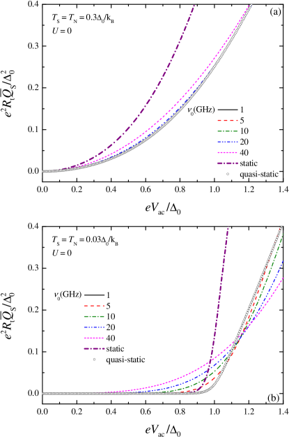
Figure 2: (color online) Normalized time-average heat current into the S electrode $\overline{Q}_{\text{S}}$ as a function of the amplitude of the AC voltage $V_{\text{ac}}$ for different values of $\nu_{0}$ at (a) high ($T=0.3\Delta_{0}/k_{\text{B}}$) and (b) low ($T=0.03\Delta_{0}/k_{\text{B}}$) temperature. The static case and the quasi-static limit are plotted for comparison. Note that in (a) the curves relative to $\nu_{0}=$10, 5 and 1 GHz coincide with the quasi-static one.

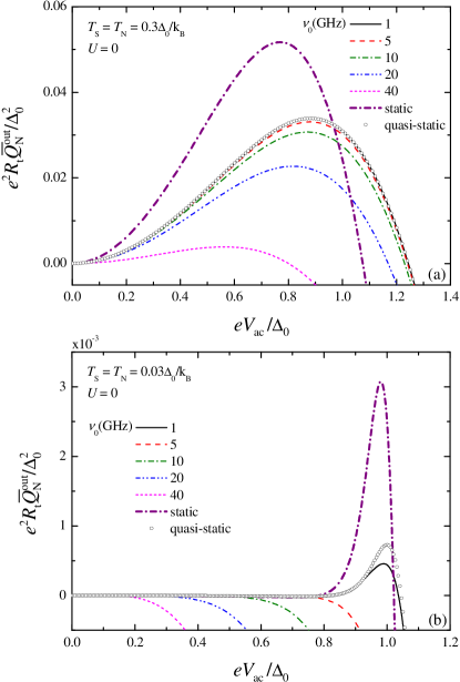
Figure 3: (color online) Normalized time-averaged heat current out of the N metal $\overline{Q}_{\text{N}}^{\text{out}}$ as a function of the amplitude of the AC voltage $V_{\text{ac}}$ for different values of frequency $\nu_{0}$ at (a) high ($T=0.3\Delta_{0}/k_{\text{B}}$) and (b) low ($T=0.03\Delta_{0}/k_{\text{B}}$) temperature. The static case and the quasi-static limit are plotted for comparison. At high temperature the quasi-static limit is a good approximation at frequencies as low as 1 GHz.

On the other hand, the photon-assisted heat current is always larger than quasi-static characteristic. To be more precise, the heat current monotonically decreases by decreasing frequency, eventually reaching the quasi-static limit for small enough $\nu_{0}$ (note that the curves relative to $\nu_{0}=1,5,10$ GHz are indistinguishable from the quasi-static one). This means that photon-assisted processes give rise to an enhancement of the heat current entering S with respect to the quasi-static situation, though remaining well below static values. Such enhancement reflects the increase in current due to photon-assisted processes tien : electrons are excited to higher energy states, thus favoring tunneling above the gap. Of course, such mechanism is more effective for small temperatures. In such a case [i.e., $T=0.03\Delta_{0}/k_{\text{B}}$, Fig. 2(b)], indeed, static and quasi-static curves present an activation-like behavior, with a switching voltage of $V_{\text{ac}}\simeq 0.9\Delta_{0}/e$ and $V_{\text{ac}}\simeq 1.0\Delta_{0}/e$, respectively, and thereby increasing almost linearly. Photon-assisted $\overline{Q}_{\text{S}}$ increases more smoothly as compared with the quasi-static case, which is approached by decreasing $\nu_{0}$.

We now consider the heat current extracted from the N electrode $\overline{Q}_{\text{N}}^{\text{out}}$, which differs from $\overline{Q}_{\text{S}}$ by the AC power $P_{\text{ac}}$ (for $U=0$) absorbed by the NIS contact [see Eqs. (31), (32)]. In Figs. 3(a) and (b) we plot $\overline{Q}_{\text{N}}^{\text{out}}$ as a function of $V_{\text{ac}}$ for several frequencies for large and small temperature, respectively. The effect of $P_{\text{ac}}$ on the behavior of the heat current is very strong, giving rise to a maximum located around $V_{\text{ac}}=\Delta_{0}/e$, and to a sign change. By increasing $V_{\text{ac}}$ the heat flow out of N increases up to the maximum and thereafter rapidly decreases to negative values (heat current enters the N electrode). For reasons given above, the maximum quasi-static heat current is always smaller than the maximum of the static one. Another effect of $P_{\text{ac}}$ is that, in this case, the photon-assisted heat current is smaller than the quasi-static characteristic. In particular, the heat current monotonically increases by decreasing frequency, eventually reaching the quasi-static limit for small enough $\nu_{0}$. Moreover, by increasing the frequency the maximum of $\overline{Q}_{\text{N}}^{\text{out}}$ moves toward smaller values of $V_{\text{ac}}$. While at large temperatures $\overline{Q}_{\text{N}}^{\text{out}}$ remains positive (implying heat extraction from the N electrode) also for frequencies slightly above 40 GHz [see Fig. 3 (a)], at low temperatures the minimum frequency for positive $\overline{Q}_{\text{N}}^{\text{out}}$ is drastically reduced (by about one order of magnitude) [see Fig. 3 (b)]. This clearly proves that photon-assisted tunneling is detrimental as far as heat extraction from the N electrode is concerned.

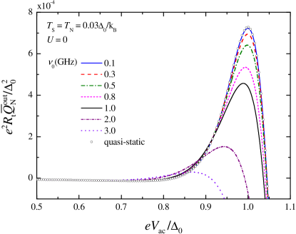
Figure 4: (color online) The same as for Fig. 3 (b) for frequencies in a smaller range. At low temperature the quasi-static limit is a good approximation for frequencies as low as 0.1 GHz.

Analogously to what happens for the charge current tien , the approach to the quasi-static limit depends on temperature. Indeed, as already mentioned in Sec. II.1, the quasi-static regime occurs at $\hbar\omega_{0}\ll k_{\text{B}}T$. The curve relative to 1 GHz differs, with respect to the quasi-static one at its maximum, by less than 0.1% at $T=0.3\Delta_{0}/k_{\text{B}}$, and by about 50% at $T=0.03\Delta_{0}/k_{\text{B}}$, where $k_{\text{B}}T\sim\hbar\omega_{0}$. Figure 4 shows the time-average $\overline{Q}_{\text{N}}^{\text{out}}$ versus $V_{\text{ac}}$ at low temperature calculated for frequencies in a smaller range. As it can be clearly seen, the quasi-static curve appears to be a good approximation for $\nu_{0}=0.1$ GHz.

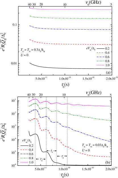
Figure 5: (color online) Normalized time-average heat current into the S electrode $\overline{Q}_{\text{S}}$ as a function of the period of the oscillations $\tau_{0}=1/\nu_{0}$ for various values of $V_{\text{ac}}$ at (a) $T=0.3\Delta_{0}/k_{\text{B}}$ and (b) $T=0.03\Delta_{0}/k_{\text{B}}$. The distance between the relative maxima at low temperature [panel (b)] is $\tau_{\Delta}=h/\Delta_{0}$.

It is now interesting to analyze the behavior of dynamic heat transport in the NIS junction for fixed amplitude of the AC voltage by plotting the heat currents as a function of the period of oscillations $\tau_{0}=1/\nu_{0}$. This is shown in Figs. 5 and 6 for $\overline{Q}_{\text{S}}$ and $\overline{Q}_{\text{N}}^{\text{out}}$, respectively. Here we set $U=0$. Both for large [$T=0.3\Delta_{0}/k_{\text{B}}$, see Fig. 5(a)] and small [$T=0.03\Delta_{0}/k_{\text{B}}$, see Fig. 5(b)] temperatures the heat current $\overline{Q}_{\text{S}}$ presents an overall decrease with $\tau_{0}$, for all values of $V_{\text{ac}}$. At small temperatures, however, the heat current shows an additional structure consisting of superimposed oscillations due to photon-assisted processes, which tend to disappear for large values of $\tau_{0}$ (small frequencies), i.e., approaching the quasi-static limit. Notably, the relative maxima turn out to be equally spaced by the time scale related to the superconducting gap, $\tau_{\Delta}=h/\Delta_{0}$. In addition we found that, at even lower temperatures, also the relative maxima are equally spaced by $\tau_{\Delta}$.

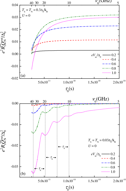
Figure 6: (color online) Normalized time-average heat current out of the N electrode $Q_{\text{N}}^{\text{out}}$ as a function of the period of the oscillations $\tau_{0}=1/\nu_{0}$ for several values of $V_{\text{ac}}$ at (a) $T=0.3\Delta_{0}/k_{\text{B}}$ and (b) $T=0.03\Delta_{0}/k_{\text{B}}$. At low temperature [panel (b)] the distance between relative minimums turn out to be $\tau_{\Delta}=h/\Delta_{0}$. In (b) the curve relative to $V_{\text{ac}}=0.2\Delta_{0}/e$ is consistent, in the scale of the figure, with zero.

Though presenting an overall enhancement with $\tau_{0}$, the behavior of the time-average heat current extracted from the N electrode $\overline{Q}_{\text{N}}^{\text{out}}$ is qualitatively similar to that of $\overline{Q}_{\text{S}}$ (see Fig. 6; note that the vertical axis is linear in this case). Note that for large temperatures $\overline{Q}_{\text{N}}^{\text{out}}$ remains positive for most of the frequency range considered, even for $V_{\text{ac}}=\Delta_{0}/e$ [see Fig. 6(a)]. For small temperatures [see Fig. 6(b)], however, the heat current is negative over nearly the whole time range. The additional structure, in this case, shows equal spacing (of magnitude $\tau_{\Delta}$) between the relative minimums, since these correspond to maximum heat absorption by S [maxima in Fig. 5(b)].

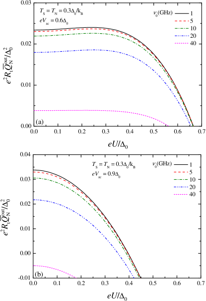
Figure 7: (color online) Normalized time-average heat current exiting the N electrode $\overline{Q}_{\text{N}}^{\text{out}}$ as a function of the DC voltage $U$ for various values of $\nu_{0}$ at (a) $V_{\text{ac}}=0.6\Delta_{0}/e$ and (b) $V_{\text{ac}}=0.9\Delta_{0}/e$. In (a) and (b) the calculations were performed by setting the temperature at $T=0.3\Delta_{0}/k_{\text{B}}$.

We now turn to the effect of a finite DC voltage $U$ combined with an AC modulation on the heat current exiting the N electrode. In Figs. 7(a) and (b), the time-average $\overline{Q}_{\text{N}}^{\text{out}}$ at large temperatures ($T=0.3\Delta_{0}/k_{\text{B}}$) is plotted as a function of $U$ for several values of frequency at $V_{\text{ac}}=0.6\Delta_{0}/e$ and $V_{\text{ac}}=0.9\Delta_{0}/e$, respectively. Figure 7(a) shows that $\overline{Q}_{\text{N}}^{\text{out}}$ is nearly constant having a weak maximum around $U\simeq 0.3\Delta_{0}/e$ almost independently of the frequency, and rapidly decreasing thereafter. By inspecting Fig. 3(a) it clearly appears that, at $T=0.3\Delta_{0}/k_{\text{B}}$, $\overline{Q}_{\text{N}}^{\text{out}}$ is maximized around $V_{\text{ac}}\approx 0.9\Delta_{0}/e$, so it seems that a finite value of $U$ just adds to the AC voltage making the heat current to move along the voltage characteristic similarly to the pure AC case. Furthermore, we note that the addition of a static DC potential to an AC modulation is not able to recover the maximum value the heat current can achieve with only the AC voltage biasing. A confirmation of this is given in the plots displayed in Fig. 7(b) which are relative to a value of $V_{\text{ac}}=0.9\Delta_{0}/e$. For such an AC voltage biasing $\overline{Q}_{\text{N}}^{\text{out}}$ does not present a constant part, and the addition of $U$ turns out to only suppress the time-average heat current. Moreover, an increase of frequency $\nu_{0}$ causes a reduction of $\overline{Q}_{\text{N}}^{\text{out}}$, even to negative values.

We finally plot in Fig. 8 the maximum value of $\overline{Q}_{\text{N}}^{\text{out}}$, obtained by spanning over $V_{\text{ac}}$, as a function of $T$ for several values of frequency. For every $\nu_{0}$ the time-average $\overline{Q}_{\text{N}}^{\text{out}}$ is a bell-shaped function presenting a maximum around $T\simeq 0.25\Delta_{0}/k_{\text{B}}$ (similarly to what happens in the static giazotto06 as well as in the quasi-static limit), which is gradually suppressed upon enhancing the frequency. By increasing the frequency the curves slightly shrink, thus reducing the temperature interval of positive heat current. Moreover, the position of the maxima tends to move to higher temperatures for intermediate frequencies (i.e., for $\nu_{0}$ below $\simeq 20$ GHZ), while they tend to move to lower temperatures in the higher range of frequencies (see for example the curve corresponding to $\nu_{0}=40$ GHz in Fig. 8).

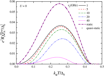
Figure 8: (color online) Normalized time-average heat current out of the N electrode $\overline{Q}_{\text{N}}^{\text{out}}$, maximized with respect to $V_{\text{ac}}$, as a function of temperature $T$ at $U=0$ for different values of frequency $\nu_{0}$. The static case and the quasi-static limit are plotted for comparison.

IV Conclusions

In this paper we have calculated the heat currents in a normal/superconductor tunnel junction driven by an oscillating bias voltage in the photon-assisted tunneling regime. We have found that the maximum heat extracted from the normal electrode decreases with increasing driving frequency. We checked that for small frequencies ($\hbar\omega_{0}\ll k_{\text{B}}T$) the photon-assisted heat current approaches the quasi-static limit, the latter being obtained by averaging the static heat current over a sinusoidal voltage cycle (relevant for sub-GHz frequencies). The suppression of the heat current by photon-assisted processes can be imputed to the AC power, dissipated at the tunnel contact, which is enhanced in the quantum regime with respect to the quasi-static limit. On the contrary, the heat current entering the superconducting electrode slightly increases with increasing frequency. We also found that, for small temperatures, the heat current as a function of the inverse of frequency presents an additional structure consisting of superimposed oscillations with a period corresponding to the time scale derived from the superconducting gap, $\tau_{\Delta}=h/\Delta_{0}$.

We want finally to briefly comment onto some implications of the above results for practically realizeable systems. We refer, for instance, to AC-driven NIS electron refrigerators operating in the regime of Coulomb blockade which were theoretically investigated in Ref. pekola07a , and experimentally demonstrated in Ref. saira . More in particular, it was shown in Ref. pekola07a that both the heat current flowing out the N island and the minimum achievable electron temperature depend on the frequency of the gate voltage as well as on the bath temperature. Our results may thus suggest the proper operating conditions in terms of frequencies and bath temperatures in order for photon-assisted tunneling not to suppress the heat current in these systems. In other words, they allow to predict a suitable range of parameters which keep the system in the quasi-static limit.

V Acknowledgments

We thank R. Fazio for careful reading of the manuscript. Partial financial support by the Russian Foundation for Basic Research grant 06-02-16002, from Academy of Finland, and from the EU funded NanoSciERA “NanoFridge” and RTNNANO projects is acknowledged.

Appendix A Static limit

To prove Eq. (10) we use that $\Phi(x)$ is analytic, therefore

$$\Phi(\epsilon-n\hbar\omega_{0})e^{-in\omega_{0}t}=\sum_{k=0}^{\infty}\frac{d^{k}\Phi}{d\epsilon^{k}}\frac{(-n\hbar\omega)^{k}}{k!}e^{-in\omega_{0}t}$$

$$=\Phi\left(\epsilon-i\hbar\frac{\partial}{\partial t}\right)e^{-in\omega_{0}t}$$

We next perform the inverse Fourier transform of the right-hand side of Eq. (10)

$$\Phi(\epsilon+\mu_{s}(t))=\sum_{n,k}J_{n}(\alpha)J_{n-k}(\alpha)\Phi(\epsilon-n\hbar\omega_{0})e^{-ik\omega_{0}t}$$

$$=\sum_{n}J_{n}(\alpha)\Phi(\epsilon-n\hbar\omega_{0})e^{-in\omega_{0}t}e^{\frac{i}{\hbar}\int_{0}^{t}eV_{ac}\cos\omega_{0}t^{\prime}\,dt^{\prime}}$$

$$=e^{\frac{i}{\hbar}\int_{0}^{t}eV_{ac}\cos\omega_{0}t^{\prime}\,dt^{\prime}}\sum_{n}\Phi\left(\epsilon-i\hbar\frac{\partial}{\partial t}\right)J_{n}(\alpha)e^{-in\omega_{0}t}$$

$$=e^{\frac{i}{\hbar}\int_{0}^{t}eV_{ac}\cos\omega_{0}t^{\prime}\,dt^{\prime}}\Phi\left(\epsilon-i\hbar\frac{\partial}{\partial t}\right)e^{-\frac{i}{\hbar}\int_{0}^{t}eV_{ac}\cos\omega_{0}t^{\prime}\,dt^{\prime}}$$

which indeed is $\Phi(\epsilon-eV_{ac}\cos\omega_{0}t)$. Here we use the expansion Eq. (6) twice.

References

• (1) A. H. Dayem and R. J. Martin, Phys. Rev. Lett. 8, 246 (1962).
• (2) C. F. Cook and G. E. Everett, Phys. Rev. 159, 374 (1967).
• (3) E. Lax and F. L. Vernon, Phys. Rev. Lett. 14, 256 (1965).
• (4) C. A. Hamilton and S. Shapiro, Phys. Rev. B 2, 4494 (1970).
• (5) T. Kommers and J. Clarke, Phys. Rev. Lett. 38, 1091 (1977).
• (6) A. A. Kozhevnikov, R. J. Schoelkopf, and D. E. Prober, Phys. Rev. Lett. 84, 3398 (2000).
• (7) A. Vaknin and Z. Ovadyahu, Europhys. Lett. 47, 615 (1999).
• (8) K. W. Yu, Phys. Rev. B 29, 181 (1984).
• (9) S. P. Kashinje and P. Wyder, J. Phys. C: Solid State Phys. 19, 3193 (1986).
• (10) F. Habbal, W. C. Danchi, and M. Tinkham, Appl. Phys. Lett. 42, 296 (1983).
• (11) J. E. Mooij and T. M. Klapwijk, Phys. Rev. B 27, 3054 (1983).
• (12) B. Leone, J. R. Gao, T. M. Klapwijk, B. D. Jackson, W. M. Laauwen, and G. de Lange, Appl. Phys. Lett. 78, 1616 (2001).
• (13) Y. Uzawa and Z. Wang, Phys. Rev. Lett. 95, 017002 (2005).
• (14) P. K. Tien, and J. P. Gordon, Phys. Rev. 129, 647 (1963).
• (15) J. R. Tucker and M. J. Feldman, Rev. Mod. Phys. 57, 1055 (1985).
• (16) J. R. Tucker, IEEE J. Quantum Electron. 15, 1234 (1979).
• (17) J. N. Sweet and G. I. Rochlin, Phys. Rev. B 2, 656 (1970).
• (18) U. Zimmermann and K. Kreck, Z. Phys. B 101, 555 (1996).
• (19) See F. Giazotto, T. T. Heikkilä, A. Luukanen, A. M. Savin, and J. P. Pekola, Rev. Mod. Phys. 78, 217 (2006), and references therein.
• (20) A. Bardas and D. Averin, Phys. Rev. B 52, 12873 (1995).
• (21) M. M. Leivo, J. P. Pekola, and D. V. Averin, Appl. Phys. Lett. 68, 1996 (1996).
• (22) M. Nahum, T. M. Eiles, and J. M. Martinis, Appl. Phys. Lett. 65, 3123 (1994).
• (23) A. M. Clark, A. Williams, S. T. Ruggiero, M. L. van den Berg, and J. N. Ullom, Appl. Phys. Lett. 84, 625 (2004).
• (24) A. M. Clark, N. A. Miller, A. Williams, S. T. Ruggiero, G. C. Hilton, L. R. Vale, J. A. Beall, K. D. Irwin, and J. N. Ullom, Appl. Phys. Lett. 86, 173508 (2005).
• (25) A. M. Savin, M. Prunnila, P. P. Kivinen, J. P. Pekola, J. Ahopelto, and A. J. Manninen, Appl. Phys. Lett. 79, 1471 (2001).
• (26) R. Leoni, G. Arena, M. G. Castellano, and G. Torrioli, J. Appl. Phys. 85, 3877 (1999).
• (27) F. Giazotto, F. Taddei, R. Fazio, and F. Beltram, Appl. Phys. Lett. 80, 3784 (2002).
• (28) F. Giazotto, F. Taddei, M. Governale, C. Castellana, R. Fazio, and F. Beltram, Phys. Rev. Lett. 97, 197001 (2006).
• (29) F. Giazotto, F. Taddei, P. D’Amico, R. Fazio, and F. Beltram, Phys. Rev. B 76, 184518 (2007).
• (30) J. P. Pekola, F. Giazotto, and O.-P. Saira, Phys. Rev. Lett. 98, 037201 (2007).
• (31) O.-P.Saira, M. Meschke, F. Giazotto, A. M. Savin, M. Möttönen, and J. P. Pekola, Phys. Rev. Lett. 99, 027203 (2007).
• (32) J. P. Pekola and F. W. J. Hekking, Phys. Rev. Lett. 98, 210604 (2007).
• (33) A. I. Larkin and Yu. N. Ovchinnikov, Zh. Eksp. Teor. Fiz. 73, 299 (1977) [Sov. Phys. JETP 46, 155 (1977)].
• (34) N. B.Kopnin, Theory of Nonequilibrium Superconductivity (Clarendon, Oxford, 2001).
• (35) J. Voutilainen, T. T. Heikkilä, and N.B. Kopnin, Phys. Rev. B 72, 054505 (2005).
• (36) R. C. Dynes, J. P. Garno, G. B. Hertel, and T. P. Orlando, Phys. Rev. Lett. 53, 2437 (1984).
• (37) J. P. Pekola, T. T. Heikkilä, A. M. Savin, J. T. Flyktman, F. Giazotto, and F. W. J. Hekking, Phys. Rev. Lett. 92, 056804 (2004).