CS22964-161: A Double-Lined Carbon- and s-Process-Enhanced Metal-Poor Binary Star

Abstract

A detailed high-resolution spectroscopic analysis is presented for the carbon-rich low metallicity Galactic halo object CS 22964-161. We have discovered that CS 22964-161 is a double-lined spectroscopic binary, and have derived accurate orbital components for the system. From a model atmosphere analysis we show that both components are near the metal-poor main-sequence turnoff. Both stars are very enriched in carbon and in neutron-capture elements that can be created in the $s$-process, including lead. The primary star also possesses an abundance of lithium close to the value of the “Spite-Plateau”. The simplest interpretation is that the binary members seen today were the recipients of these anomalous abundances from a third star that was losing mass as part of its AGB evolution. We compare the observed CS 22964-161 abundance set with nucleosynthesis predictions of AGB stars, and discuss issues of envelope stability in the observed stars under mass transfer conditions, and consider the dynamical stability of the alleged original triple star. Finally, we consider the circumstances that permit survival of lithium, whatever its origin, in the spectrum of this extraordinary system.

1 INTRODUCTION

The chemical memory of the Galaxy’s initial elemental production in short-lived early-generation stars survives in the present-day low-mass, low metallicity halo stars showing starkly contrasting abundance distributions. Metal-poor stars have been found with order-of-magnitude differences in lithium contents, large ranges in $\alpha$-element abundances (from [Mg,Si,Ca,Ti/Fe]  $<$ 0 to $\sim$+1), non-solar Fe-peak ratios, and huge bulk variations in neutron-capture ($n$-capture) abundances.

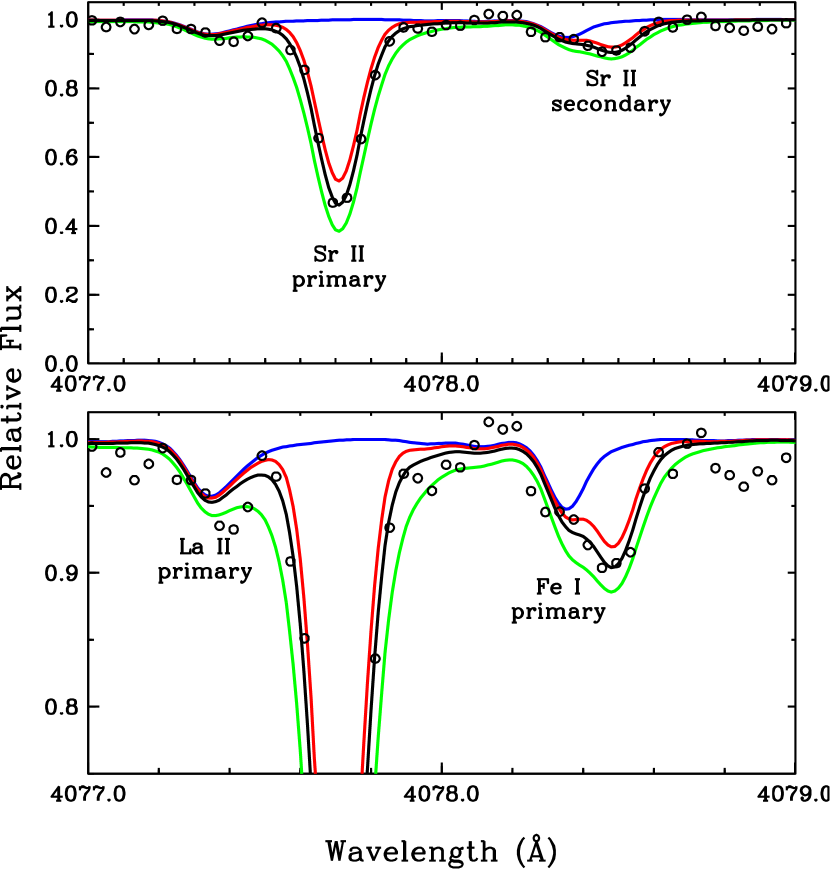
Figure 6: Observed and synthetic spectra of the Sr II 4077.71 Å line in observation 13817 of CS 22964-161 ($\Delta V_{R}$ $\simeq$ 58.09 km s^-1). The top spectrum shows the full relative flux scale, and the bottom spectrum covers just the relative flux region above 0.75. The wavelength scale is at rest velocity for the primary star. The observed spectrum is depicted with open circles. The blue line represents a synthetic spectrum computed without any contribution from Sr. The black line shows the best overall fit to primary and secondary Sr II features: log $\epsilon$(Sr) = 0.98 and 0.78, respectively. The red and green lines indicate syntheses for each star that are 0.5 dex smaller and larger, respectively, than the best fits.

One anomaly can be easily spotted in medium-resolution (R $\equiv$ $\lambda/\Delta\lambda$ $\simeq$ 2000) spectroscopic surveys of metal-poor stars: large star-to-star variations in CH G-band strength, leading to similarly large carbon abundance ranges. Carbon-enhanced metal-poor stars (hereafter CEMP $\equiv$ [C/Fe] $\gtrsim$ +1) are plentiful at metallicities [Fe/H] $<$ $-$2, with estimates of their numbers ranging from $\simeq$14% (Cohen et al. 2005) to $\gtrsim$21% (Lucatello et al. 2006). The large carbon overabundances are mainly (but not always) accompanied by large $n$-capture overabundances, which are usually detectable only at higher spectral resolution (R $\gtrsim$ 10,000). In all but one of the CEMP stars discovered to date, the $n$-capture abundance pattern has its origin in slow neutron-capture synthesis (the $s$-process). The known exception is CS 22892-052 (e.g., Sneden et al. 2003a and references therein), which has [C/Fe] $\sim$ +1 but an $n$-capture overabundance distribution clearly consistent with a rapid neutron-capture (the $r$-process) origin. Properties of CEMP stars have been summarized recently in a large-sample high-resolution survey by Aoki et al. (2007). They conclude in part that the abundances of carbon and ($n$-capture) barium are positively correlated (their Figure 6), pointing to a common nucleosynthetic origin of these elements in many CEMP stars.

CS 22964-161 was first noted in the “HK” objective prism survey of low metallicity halo stars (Beers, Preston, & Shectman 1992, hereafter BPS92). Using as metallicity calibration the strength of the Ca II K line, BPS92 estimated [Fe/H] $\simeq$ $-$2.62. They also found CS 22964-161 to be one of a small group of stars with unusually strong CH G-bands (see their Table 8). Recently, Rossi et al. (2005) analyzed a moderate resolution spectrum of this star. From the extant BVJK photometry and distance estimate they suggested that CS 22964-161 is a subgiant: $T_{\rm eff}$ = 5750 K and log g = 3.3. Two metallicity estimates from the spectrum were in agreement at [Fe/H] = $-$2.5, and three independent approaches to analysis of the overall CH absorption strength suggested a large carbon abundance, [C/Fe] = +1.1.

We observed CS 22964-161 as part of a high resolution survey of candidate low-metallicity stars selected from BPS92. When we discovered that the star shows very strong features of CH and $n$-capture species Sr II and Ba II, similar to many binary blue metal-poor (BMP) stars (Sneden, Preston, & Cowan 2003b), we added it to a radial velocity monitoring program. Visual inspection of the next observation showed two sets of spectral lines, and so an intensive monitoring program was initiated on the du Pont and Magellan Clay telescopes at Las Campanas Observatory. In this paper we present our orbital and abundance analyses of CS 22964-161. Radial velocity data and the orbital solution are given in §2, and broadband photometric information in §3. We discuss the raw equivalent width measurements for the combined-light spectra and the extraction of individual values for the CS 22964-161 primary and secondary stars in §4. Determination of stellar atmospheric parameters is presented in §5, followed by abundance analyses of the individual stars in §6 and of the CS 22964-161 system in §7. Interpretation of the large lithium, carbon, and $s$-process abundances in primary and secondary stars is discussed in §8. Finally, we speculate on the nature of former asymptotic giant branch (AGB) star that we suppose was responsible for creation of the unique abundance mix of the CS 22964-161 binary in §9.

2 RADIAL VELOCITY OBSERVATIONS

We obtained spectroscopic observations of CS 22964-161 with the Clay 6.5-m MIKE (Bernstein et al. 2003) and du Pont 2.5-m echelle (R $\simeq$ 25,000) spectrographs. Properties of the two spectrographs are presented at the LCO website. The Clay MIKE data have $R$ $\equiv$ $\lambda/\delta\lambda$ and continuous spectral coverage for 3500 Å $\lesssim$ $\lambda$ $\lesssim$ 7200 Å. The du Pont data have R $\simeq$ 25,000, and out of the large spectral coverage of those data we used the region 4300 Å $\lesssim$ $\lambda$ $\lesssim$ 4600 Åfor velocity measurements. Exposure times ranged from 1245 to 3500 seconds on the Clay telescope and 3000 to 4165 seconds on the du Pont telescope. The observations generally consist of two exposures flanked by observations of a thorium-argon hollow-cathode lamp.

The Magellan observations were reduced with pipeline software written by Dan Kelson following the approach of Kelson (2003, 2006). Post-extraction processing of the spectra was done within the IRAF ECHELLE package. The du Pont observations were reduced completely with IRAF ECHELLE software.

Velocities were initially measured with the IRAF FXCOR package using MIKE observations of HD 193901 as a template, and a preliminary orbit was derived. The three MIKE observations of CS 22964-161 obtained at zero velocity crossing (phase $\simeq$ 0.11) were then averaged together to define a new template, hereafter called the syzygy spectrum. This spectrum has a total integration time of 10215 sec and S/N $>$ 160 at 4260 Å. We remeasured the velocities using this new template with the TODCOR algorithm (Zucker & Mazeh 1994). The cross-correlations covered the wavelength interval 4130 Å $<$ $\lambda$ $<$ 4300 Å. The syzygy spectrum was also used extensively in our abundance analysis (§6).

The radial velocity data were fit with a non-linear least squares solution. We chose to fit to only the higher resolution and higher S/N Magellan data, using the du Pont data to confirm the orbital solution. The observations are presented in Table 1 which lists the heliocentric Julian Date (HJD) of mid-exposure, the velocities of the primary and secondary components, and the orbital phases of the observations. The adopted orbital elements are listed in Table 2 and the adopted orbit is plotted in Figure 1. Of particular importance to later discussion in this paper are the derived masses: $M_{p}~{}sin^{3}~{}i$ = 0.773 $\pm~{}$0.009 $M_{\odot}$ and $M_{s}~{}sin^{3}~{}i~{}$ = 0.680 $\pm$ 0.007 $M_{\odot}$; the orbital inclination cannot be derived from our data.

We will discuss the velocity residuals to the orbital solution further in §9. Hereafter, references to individual spectra will be by the HJD of Table 1, e.g., the spectrum obtained with Magellan MIKE on HJD 13817.90625 will be called “observation 13817”.

3 PHOTOMETRIC OBSERVATIONS

Preston, Shectman, & Beers (1991) list $V$ = 14.41, $B-V$ = 0.488, and $U-B$ = $-$0.171 for CS 22964-161 based on a single photoelectric observation on the du Pont telescope. New CCD observations of this star were obtained with the du Pont telescope on UT 28 May 2006. The data were calibrated with observations of the Landolt standard field Markarian A (Landolt 1992). Observations of the standards and program object were taken at an airmass of $\sim$1.12, and we used standard extinction coefficients in the reductions. We derived $V$ = 14.43 and $B-V$ = 0.498 for CS 22964-161. Old and new photometric data are consistent with the typical $\sim$1% observational uncertainties in magnitudes, so we adopt final values of $V$ = 14.42 and $B-V$ = 0.49.

The ephemeris given in Table 2 predicts a primary eclipse at HJD2454315.045 (2 August 2007, UT 13.08 hours) and a secondary eclipse at HJD 2454344.453 (31 August 2007, UT 22.87 hours). CS 22964-161 was monitored on the nights of 2/3 August 2007 and 31 August/1 September using the CCD camera on the Swope telescope at Las Campanas. Observations were obtained approximately every hour with a $V$ filter. No variations in the $V$ magnitude of CS 22964-161 in excess of 0.02 magnitudes were detected.

4 EQUIVALENT WIDTH DETERMINATIONS

A double-line binary spectrum is a complex, time-variable mix of two sets of absorption lines and two usually unequal continuum flux levels. Following Preston (1994) we define observed equivalent widths $EW_{o}$ to be those measured in the combined-light spectra, and true equivalent widths $EW_{t}$ to be those of each star in the absence of its companion’s contribution. If the primary-secondary velocity separation is large, one can attempt to measure observed $EW$s of primary and secondary stars independently. If this can be accomplished then true $EW$s can be computed from knowledge of the relative flux levels of the stars. In practice the derivation of true $EW$s is complex and subject to large uncertainties.

In Figure 2 we illustrate the difficulties in deducing observed $EW$s for each star from the observed CS 22964-161 composite spectra. Recall that in the syzygy spectrum (the co-addition of three individual observations), there is no radial velocity separation, or $\Delta V_{R}$ $\simeq$ 0 km s^-1. The primary and secondary spectral lines coincide in wavelength, producing the simple spectrum shown at the bottom of Figure 2. In contrast, the middle spectrum in this figure was generated from spectra in which the velocity separation was large enough for primary and secondary lines to be resolved (hereafter called velocity-split spectra). We co-added three of these spectra that have similarly large velocity differences, $\Delta V_{R}$ $\simeq$ 60 km s^-1 (observations 13580, 60.12 km s^-1; 13817, 58.09 km s^-1; and 13832, 62.40 km s^-1; Table 1). The weaker, redshifted secondary absorption lines are obvious from comparison of this and the syzygy spectrum.

Identification of the secondary absorption lines is clarified by inspection of the top spectrum in Figure 2. We created this artificial spectrum to mimic the appearance of the secondary by diluting the observed syzygy spectrum with addition of a constant three times larger than the observed continuum, and shifting that spectrum redward by 60 km s^-1. In this line-rich wavelength domain, the velocity shift yields a few cleanly separated primary and secondary absorption features. For example, 4199.11 Å Fe I in the primary becomes 4199.95 Å in the secondary, and observed $EW$s of both stars can be measured. More often however, secondary lines are shifted to wavelengths very close to other primary lines, destroying the utility of both primary and secondary features. An example of this is the Fe I 4198.33 Å line, which at $\Delta V_{R}$ $\simeq$ 60 km s^-1 becomes 4199.17 Å for the secondary star, which contaminates the Fe I 4199.11 Å line of the primary star. The various blending issues, combined with the intrinsic weakness of the secondary spectrum, yield few spectral features with clean $EW$ values for both primary and secondary stars.

4.1 Equivalent Widths from Comparison of Syzygy and Velocity-Split Spectra

In view of the blending issues outlined above, we derived the observed $EW$s through a spectrum difference technique. On the mean syzygy spectrum, we measured $EW_{o,tot}=EW_{o,p}+EW_{o,s}$, where subscripts $o$ denotes an observed $EW$, and $p$ and $s$ denote primary and secondary stars. On five spectra with large primary-secondary velocity separations (13580, 13585, 13587, 13817, 13834) we measured the primary star lines, $EW_{o,p}$. These five independent values were then averaged, and then the secondary star’s values were computed as $EW_{o,s}=EW_{o,tot}-<EW_{o,p}>$. In this procedure we attempted to avoid primary lines that would have significant contamination by secondary lines in the velocity-split spectra.

The observed $EW$ values are given in Table 3, along with the line excitation potentials and transition probabilities. In this table we also include the atomic data for lines from which abundances ultimately derived from synthetic spectrum rather than $EW$ computations. For one estimate of the uncertainty in our $EW$ measurement procedure, we computed standard deviations for the primary-star measurements of each line $\sigma EW_{o,p}$. The mean and median of these values for the whole line data set were 5.2 and 4.1 mÅ, respectively. The uncertainties in $EW_{o,tot}$ are expected to be smaller because the syzygy spectrum is the mean of three individual observations and is thus of higher S/N. Therefore we take 4$-$5 mÅ as an estimate of the uncertainty in $EW_{o,s}$ values determined in the subtraction procedure.

For a few very strong transitions the secondary lines are deep enough to cleanly detect when they split away from the primary lines. We have employed these to assess the reliability of the $EW$s derived by the subtraction method described above. In Figure 3 we show a comparison of $EW_{o,s}$ values given in Table 3 for seven lines that we measured on up to six velocity-split spectra (the five named in the previous paragraph plus 13832, which was not used in the subtraction procedure). Taking the means of the $EW_{o,s}$ measurements of each line and comparing them to the subtraction-based values of Table 3, the average difference for the seven lines is 0.8 mÅ with a scatter $\sigma$ = 3.5 mÅ (the median difference is 0.6 mÅ). This argues that in general the individual $EW_{o,s}$ values agree with the $EW_{o,s}$ subtraction-based ones.

Derivation of true $EW$s depends on knowledge of the relative luminosities of primary and secondary stars. Formally, from Preston’s (1994) equations 4$-$5, we have $EW_{p,t}=EW_{p,o}(1+l_{s}/l_{p})$, and $EW_{s,t}=EW_{s,o}(1+l_{p}/l_{s})$, where subscript $t$ represents the true $EW$, and $l$ denotes an apparent luminosity. The luminosity ratios will be wavelength-dependent if the two stars are not identical in temperature. For the entire line data set, ignoring weaker primary lines (those with $EW_{p,o}$ $<$ 25.0 mÅ), we calculated a median equivalent width ratio ($EW_{p,o}/EW_{s,o}$) = 5.2. Inspection of the velocity-split spectra suggested that relative line strengths in the secondary spectrum were not radically different from those of the primary spectrum. Therefore we concluded that the spectral types of the stars are not too dissimilar and therefore we concluded that to first approximation $EW_{p,t}$ $\sim$ $EW_{s,t}$. This assumption then leads to $EW_{p,o}/EW_{s,o}$ $\sim$ $l_{p}/l_{s}$ $\sim$ 5.

To account roughly for the small derived temperature difference (see §5) we finally adopted $l_{p}/l_{s}$ = 5.0 in the photometric $V$ bandpass ($\lambda\simeq 5500$ Å), and increased the ratio linearly by a small amount with decreasing wavelength. Thus in the $B$ bandpass ($\lambda\simeq 4400$ Å) we used $l_{p}/l_{s}$ = 5.6. Final true $EW$ values using this prescription are given in Table 3. The correction factors between observed and true $EW$s were approximately 1.2 and and 6.0 for primary and secondary stars in the $V$ spectral region, and the disparity in these factors is larger at $B$. Clearly the $EW_{p,t}$ values of Table 3 are much more reliably determined than the $EW_{s,t}$ ones.

5 STELLAR ATMOSPHERE PARAMETERS

5.1 Derivation of Parameters

We used the observed $B-V$ color and minimum masses for the binary together with the Victoria-Regina stellar models (VandenBerg, Bergbusch, & Dowler 2006), to estimate initial model atmospheric parameters for the component stars of CS 22964-161. We adopted $B-V$ = 0.49 from §3 and $E(B-V)$ = 0.07 (BPS92; a value we also estimate employing the dust maps of Schlegel, Finkbeiner, & Davis 1998) to obtain $(B-V)_{0}$ = 0.42. We assumed initially that $sin^{3}~{}i$ $\simeq$ 1.0 for the binary orbit and thus $M_{p}$ = 0.773 $M_{\odot}$ and $M_{s}$ = 0.680 $M_{\odot}$, as derived in §2. We interpolated the Victoria-Regina models computed for [Fe/H] = $-$2.31, [$\alpha$/Fe] = +0.3, and $Y$ = 0.24, to obtain evolutionary tracks for these masses. These tracks were used to derive $B-V$ colors and luminosity ratios for the component stars. We adopted starting values of $T_{\rm eff}$, log g, and $l_{p}/l_{s}$ where the tracks give $B-V$ = 0.42 for the combined system. These values were $T_{\rm eff}$_,p = 6050 K, $T_{\rm eff}$_,s = 5950 K and log g_p = 3.6, log g_s = 4.2. The luminosity ratios using these parameters were $l_{p}/l_{s}~{}(B)$ = 8.65 and $l_{p}/l_{s}~{}(V)$ = 8.39, somewhat larger than implied by our spectra.

Final model atmospheric parameters were found iteratively from the $EW$ data for the two stars. We employed the LTE line analysis code MOOG (Sneden 1973) and interpolated model atmospheres from the Kurucz (1998) grid computed with no convective overshoot (as recommended by Castelli, Gratton, & Kurucz 1997, and by Peterson, Dorman, & Rood 2001).

We began by using standard criteria to estimate the model parameters of the CS 22964-161 primary: (a) for $T_{\rm eff}$, no trend of derived Fe I individual line abundances with excitation potential; (b) for $v_{\rm t}$, no trend of Fe I abundances with $EW$; (c) for log g, equality of mean Fe I and Fe II abundances (for no other element could we reliably measure lines of the neutral and ionized species); and (d) for model metallicity [M/H], a value roughly compatible with the Fe and $\alpha$ abundances. These criteria could be assessed reliably for the primary star because it dominates the combined light of the two stars. In the top panel of Figure 4 we illustrate the line-to-line scatter and (lack of) trend with wavelength of the primary’s Fe I and Fe II transitions. With iteration among the parameters we derived ($T_{\rm eff}$_,p, log g_p, $v_{\rm t}$_p, [M/H]_p) = (6050$\pm$100 K, 3.7$\pm$0.2, 1.2$\pm$0.3 km s^-1, $-$2.2$\pm$0.2).

To estimate model parameters for the secondary we assumed that derived [Fe/H] metallicities and abundance ratios of the lighter elements (Z $\leq$ 30) in the primary and secondary stars should be essentially identical if they were formed from the same interstellar cloud. Iteration among several sets of ($T_{\rm eff}$_,s, log g_s) pairs was done until [Fe/H]_s $\simeq$ [Fe/H]_p and Fe ionization equilibrium for the secondary was achieved. Given the weakness of the secondary spectrum and the resulting large correction factors used to calculate $EW_{s,t}$ from $EW_{s,o}$ values, it is not surprising that the spectroscopic constraints on the secondary parameters were weak. This is apparent from the adopted Fe abundances displayed in the bottom panel of Figure 4. The $\sigma$ values for individual line abundances were about three times larger for the secondary than the primary (Table 4), and number of transitions was substantially smaller (e.g., we measured seven Fe II lines for the primary but only three for the secondary).

We adopted final model parameters of ($T_{\rm eff}$_,s, log g_s, $v_{\rm t}$_s, [M/H]_s) = (5850 K, 4.1, 0.9 km s^-1, $-$2.2). Model uncertainties for the secondary were not easy to estimate and, of course, were tied to our opening assumption that the two stars have identical overall metallicities and abundance ratios. Thus with [M/H]_p $\equiv$ [M/H]_s, the uncertainties in $T_{\rm eff}$, log g, and $v_{\rm t}$ of the secondary are approximately double their values quoted above for the primary. Thus caution is obviously warranted in interpretation of the model parameters of the CS 22964-161 secondary.

5.2 Comparison to Evolutionary Tracks

The well-determined $T_{\rm eff}$_,p and log g_p values can be used with the mass and luminosity ratios of the stars to provide an independent estimate of $T_{\rm eff}$_,s and log g_s. Standard relations $L\propto R^{2}\mbox{$T_{\rm eff}$}^{4}$ and $g\propto M/R^{2}$ lead to

$${\rm log}(L_{s}/L_{p})={\rm log}(l_{s}/l_{p})={\rm log}(M_{s}/M_{p})+4\times{\rm log}(\mbox{$T_{\rm eff}$}_{,s}/\mbox{$T_{\rm eff}$}_{,p})-{\rm log}(g_{s}/g_{p})$$

Taking an approximate average luminosity ratio to be $l_{p}/l_{s}$ $\simeq$ 5.3, adopting $M_{s}/M_{p}$ = 1.15 (Table 2) and assuming $T_{\rm eff}$_,p = 6050 K and log g_p = 3.7 from above, we get a predicted temperature-gravity relationship log g_s $\simeq$ 4$\times$log($T_{\rm eff}$_,s) $-$ 10.8 .

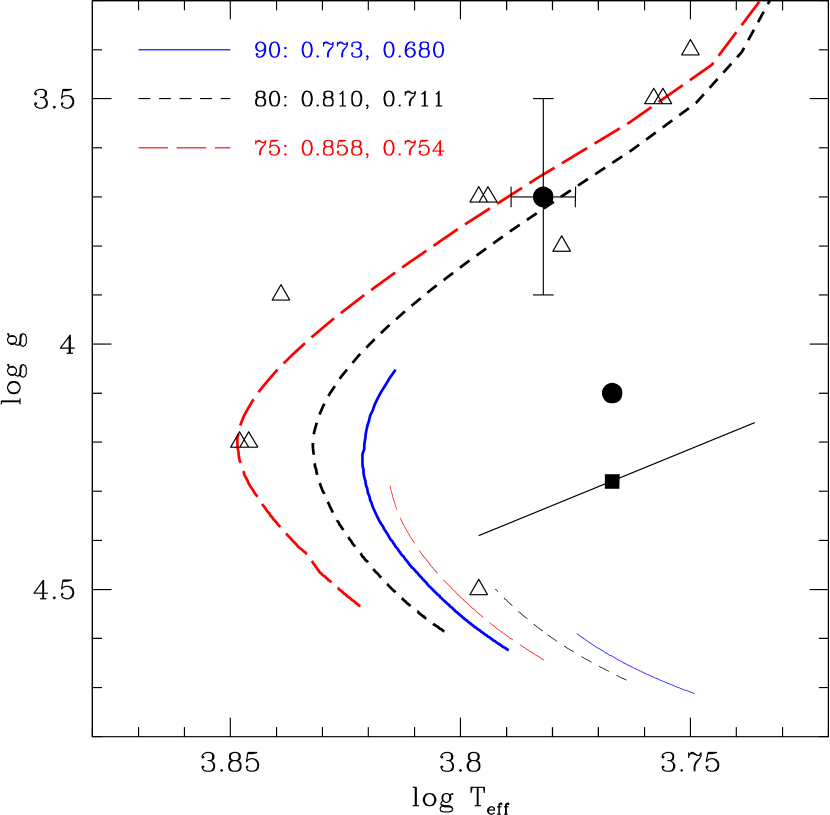
Figure 5: Evolutionary tracks (VandenBerg et al. 2006) and CEMP data plotted in the log $T_{\rm eff}$ $-$ log g plane near the metal-poor main-sequence turnoff. The chosen tracks correspond to three different inclinations of the binary; heavy and light lines are for the primary and secondary, respectively. A full track covers an age range of 4 to 14 Gyr. The figure legend identifies the masses of the tracks for three different CS 22964-161 orbital $sin\ i$ choices, using the notation ($sin\ i$: $M_{p}$, $M_{s}$). Filled circles represent the CS 22964-161 primary and secondary (log $T_{\rm eff}$, log g) values derived from the spectroscopic analysis (§5.1). The plotted error bars for the primary are also from the spectroscopy. The square shows the secondary parameters from the dimensional analysis described in §5.2, The line about this point corresponds to $\Delta$$T_{\rm eff}$ = $\pm$400 K. The triangles represent CEMP stars from the literature; see §5.2 for details. The triangles for three pairs of stars with identical temperatures and gravities have been shifted apart from each other for display purposes.

In Figure 5 we show the very metal-poor main sequence turnoff region of the H-R diagram in (log $T_{\rm eff}$, log g) units. The Victoria-Regina evolutionary tracks (VandenBerg et al. 2006; [Fe/H] = $-$2.31, [$\alpha$/Fe] = +0.3, and $Y$ = 0.24) discussed in §5.1 are again employed. However, the unknown binary orbital inclination of CS 22964-161 cannot be ignored here. Therefore we have plotted the tracks for three pairs of masses corresponding to assumed $sin\ i$ values of 90^∘, 80^∘, and 75^∘. Also plotted is a straight line representing the CS 22964-161 secondary star temperature-gravity equation derived above.

The CS 22964-161 primary and secondary and ($T_{\rm eff}$, log g) positions are indicated with filled circles in Figure 5. We also add data indicated with open triangles from CEMP high resolution spectroscopic studies for C-rich stars of similar metallicity, taken here to be [Fe/H] = $-$2.4 $\pm$ 0.4. The studies include those of Aoki et al. (2002), Sneden et al. (2003b), and Cohen et al. (2006). If $T_{\rm eff}$_,s = 5850 K from the spectroscopic analysis then the temperature-gravity relationship from above predicts log g_s = 4.3 (indicated by a filled square in the figure). Our spectroscopic value of log g_s = 4.1 lies well within the uncertainties of both estimates.

Given the apparently anomalous position of the CS 22964-161 secondary in Figure 5, it is worth repeating its abundance analysis using atmospheric parameters forced to approximately conform with the evolutionary tracks. This is equivalent to attempting a model near the high temperature, high gravity end of its predicted relationship shown in the figure. Therefore we computed abundances for a model with parameter set ($T_{\rm eff}$_,s, log g_s, [M/H]_s) = (6300 K, 4.5, $-$2.2). Assumption of a secondary microturbulent velocity $v_{\rm t}$_s = $v_{\rm t}$_p =  $-$1.2 km s^-1, yields log $\epsilon$(Fe) = 5.45 and 5.27 from Fe I and Fe II lines, respectively. These values are substantially larger than the mean abundances for primary and secondary given in Table 4, log $\epsilon$(Fe) = 5.11. This is in agreement with expectations of a larger derived metallicity from the 350 K increase in $T_{\rm eff}$_,s for this test. However, the Fe I line abundances for this hotter model also exhibit an obvious trend with $EW$. This problem could be corrected by increasing $v_{\rm t}$ to 2.4 km s^-1, and then we get log $\epsilon$(Fe) = 5.18 and 5.15 from Fe I and Fe II lines, very close to our final adopted Fe abundances for the secondary. However, it is difficult to reconcile such a large $v_{\rm t}$ with the much smaller value determined with more confidence in the primary, as well as standard values determined in many literature studies of near-turnoff stars.

6 ABUNDANCES OF THE INDIVIDUAL STARS

With the $EW$ data of Table 3 and the interpolated model atmospheres described in §5, we determined abundances of a few key elements whose absorption lines are detectable in both primary and secondary observed spectra. These abundances are given in Table 4. They suggest that in general the abundance ratios of all elements in the two stars agree to within the stated uncertainties. Both stars are relatively enriched in the $\alpha$ elements: $<$[Mg,Ca,Ti/Fe]${}_{p}>$ $\simeq$ +0.4 and $<$[Mg,Ca,Ti/Fe]${}_{s}>$ $\simeq$ +0.3. Both stars have solar-system Ni/Fe ratios, probably no substantial depletions or enhancements of Na (special comment on this element will be given in §7), and large deficiencies of Al. All these abundance ratios are consistent with expectations for normal metal-poor Population II stars.

More importantly, we find very large relative abundances of C, Sr, and Ba ([X/Fe] = +0.5 to +1.5; Table 4) in both primary and secondary stars of the CS 22964-161 system. For Sr and Ba abundances we first used the $EW$ subtraction technique, which suggested roughly equal abundances of these elements in both stars. We confirmed and strengthened this result through synthetic spectrum computations of the strong Sr II 4077.71, 4215.52 Å and the Ba II 4554.04 Å lines in the six velocity-split spectra. To produce the binary syntheses we modified the MOOG line analysis code to compute individual spectra for primary and secondary stars, then to add them after (a) shifting the secondary spectrum in wavelength to account for the velocity difference between the stars, and (b) weighting the primary and secondary spectra by the appropriate luminosity ratio.

In Figure 6 we show the resulting observed/synthetic binary spectrum match for the Sr II 4077.71 Å line in observation 13817. The absorption spectrum of the secondary star is shifted by +58.1 km s^-1 (+0.79 Å), in agreement with the observed feature in Figure 6. The depth of the Sr II line in the secondary is weak, as expected due to the luminosity difference between the two stars ($l_{p}/l_{s}$ $\simeq$ 6) at this wavelength. Note also in Figure 6 the relative insensitivity of the feature to abundance changes for the secondary, even with the large ($\pm$0.5 dex) excursions in its assumed Sr content. This occurs because the Sr II line is as saturated in the secondary as it is in the primary, but the central intensity of the unsmoothed spectrum is $\sim$0.2 of the continuum. Thus after the secondary’s spectrum is diluted by the much larger flux of the primary, a weak line that is relatively insensitive to abundance changes ensues in the combined spectrum (and a naturally weaker line in the secondary simply becomes undetectable in the sum).

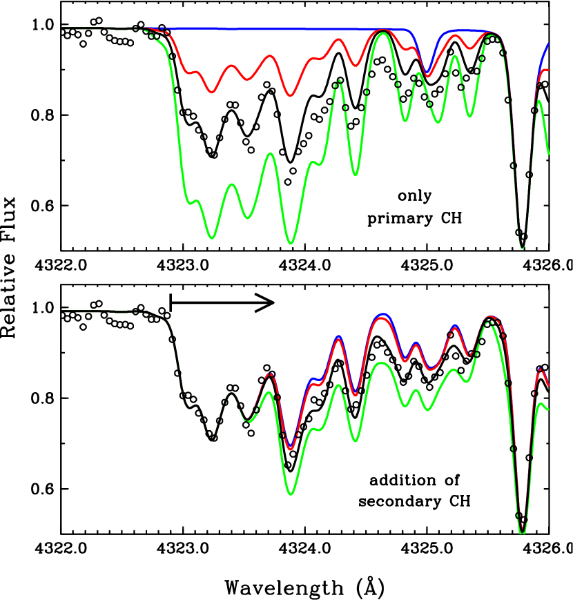
Figure 7: Observed and synthetic spectra of the CH G-bandhead in CS 22964-161. The observation is 13817, for which $\Delta V_{R}$ = 58.09 km s^-1. Open circles represent the observed spectrum. In the top panel only the contribution of the primary star to this blend is considered. The abundances of the synthetic spectra, in order of increasing CH strength, are log $\epsilon$(C)_p = $-\infty$, 7.24, 7.64, and 8.04 (the blue, red, black, and green lines, respectively). In the bottom panel, the abundance of the primary is fixed at log $\epsilon$(C)_p = 7.64, and that of the secondary is, again in order of increasing CH strength, log $\epsilon$(C)_s = $-\infty$, 6.44, 7.44, and 8.44. An arrow indicates the wavelength offset between primary and secondary stars of this observation.

In Figure 7 we illustrate the appearance of a small portion of the CH G-band $A^{\rm 2}\Delta-X^{\rm 2}\Pi^{+}$ Q-branch bandhead in the observed combined-light spectra with a large velocity split. This portion of the G-band has a sharp blue edge; the central wavelength of the first line is 4323.0 Å. With $\Delta V_{R}$ = +58.1 km s^-1, the left edge of the secondary’s bandhead begins at 4323.8 Å, as indicated in the bottom panel of Figure 7. In the top panel we show attempts to match the observed bandhead with synthetic spectra that include only CH lines of the primary star. When the spectral interval $\lambda$ $<$ 4324.8 Å is fit well, observed absorption is clearly missing at longer wavelengths in the synthetic spectrum. This is completely solved by the addition of the secondary’s CH bandhead, at a comparable C abundance level to that of the primary, as shown in the bottom panel.

It is very difficult to derive reliable abundances in the CS 22964-161 secondary even for the strong features illustrated here. Nevertheless, it is clear that both components of this binary have substantial overabundances of C and $n$-capture elements Sr and Ba. Within the uncertainties of our analysis, the overabundance factors for these elements appear to be the same. Enhanced C accompanies $s$-process synthesis of $n$-capture elements during partial He-burning episodes of low/intermediate-mass stars, and the joint production of these elements is evident in the observed abundances of a number of BMP stars such as CS 29497-030 (Sneden et al. 2003b; Ivans et al. 2005). However, a substantial C overabundance has also been seen in the $r$-process-rich star CS 22892-052 (Sneden et al. 2003a). The Sr and Ba abundances determined to this point cannot distinguish between possible $n$-capture mechanisms that created the very heavy elements in CS 22964-161.

7 ABUNDANCES FROM THE SYZYGY SPECTRUM

To gain further insight into the $n$-capture element abundance distribution we returned to the higher S/N mean syzygy spectrum. Preston et al. (2006b) argued that the relative strengths of La II and Eu II lines can easily distinguish $s$-process dominance (stronger La features) from $r$-process dominance (stronger Eu); see their Figure 1. In panels (a) and (b) of Figure 8 we show the same La and Eu lines discussed by Preston et al.; the greater strength of the La feature is apparent.

We computed a mean $EW$ from La II lines at 3988.5, 3995.7, 4086.7, and 4123.2 Å, and a mean $EW$ from Eu II lines at 3907.1, 4129.7, and 4205.1 Å for a few warm metal-poor stars with $n$-capture overabundances. The resulting ratio $<EW_{\rm La}>$/$<EW_{\rm Eu}>$ $\simeq$ 0.5 for the $r$-process-rich red horizontal-branch star CS 22886-043 (Preston et al. 2006a), $\simeq$ 2.8 for the $s$-process-rich RR Lyrae TY Gruis (Preston et al. 2006a), and $\simeq$ 2.7 for the $r$+$s$ BMP star CS 29497-030 (Ivans et al. 2005). For CS 22964-161 we found $<EW_{\rm La}>$/$<EW_{\rm Eu}>$ $\simeq$ 2.7, an unmistakable signature of an $s$-process abundance distribution.

For a more detailed $n$-capture element distribution for CS 22964-161 we computed synthetic spectra of many transitions in the syzygy spectrum. We used the same binary synthesis version of the MOOG code that was employed for the velocity-split spectra shifted to $\Delta V_{R}$ = 0 km s^-1 (as described in §6). For these computations it was also necessary to assume that log $\epsilon$(X)_p = log $\epsilon$(X)_s for all elements X. We also derived abundances of a few lighter elements of interest with this technique. It should be noted that since the primary star is 4–6 times brighter than the secondary, abundances derived in this manner mostly apply to the primary.

In Table 5 we give the abundances for the CS 22964-161 binary system. For elements with abundances determined for the individual stars as discussed in §6, we also give estimates of their “system” abundances in this table. These mean abundances were computed from the entries in Table 4, giving both the abundances and their uncertainties ($\sigma$) of the primary star five times more weight than those of the secondary. For elements with abundances derived from synthetic spectra of the syzygy spectrum, the abundances and $\sigma$ values are means of the results from individual lines, wherever possible. For several of these elements only one transition was employed. In these cases we adopted $\sigma$ = 0.20 or 0.25, depending on the difficulties attendant in the synthetic/observed spectrum matches. In the next few paragraphs we discuss the analyses of a few species that deserve special comment.

Li I: The resonance transition at 6707.8 Å was easily detected in all CS 22964-161 spectra, with $EW_{o,tot}$ $\simeq$ 24.5 mÅ from the syzygy data. Our synthesis included only ⁷Li, but with its full hyperfine components. The resolution and S/N combination of our spectra precluded any meaningful search for the presence of ⁶Li. Reyniers et al. (2002) have shown that the presence of a Ce II transition at 6708.09 Å can substantially contaminate the Li feature in $n$-capture-rich stars. However, in our spectra the Ce line wavelength is too far from the observed feature, and our syntheses indicated that the Ce abundance would need to be about two orders of magnitude larger than our derived value (Table 5) to produce measurable absorption in the CS 22964-161 spectrum.

We attempted to detect the secondary Li I line in two different ways. First, we applied the subtraction technique (§4) to this feature. However, the six velocity-split spectra yielded $EW_{o,p}$ = 23.5 mÅ with $\sigma$ = 3.5 mÅ (consistent with typical uncertainties for this technique). Thus the implied $EW_{o,s}$ = 1.0 mÅ is consistent with no detection of the secondary’s line. Second, we co-added the velocity-split spectra after shifting them to the rest system of the secondary. A very weak ($EW_{o,s}$ $\simeq$ 4 mÅ) line appears at $\lambda$ = 6707.9 Å, about 0.1 Å redward of the Li I feature centroid. We computed synthetic spectra assuming that the observed line is Li, and derived log $\epsilon$(Li) $\simeq$ +2.0 with an estimated uncertainty of $\pm$0.2 from the observed/synthetic fit. This abundance is fortuitously close to the system value, but we do not believe that the present data warrant a claim of Li detection in the CS 22964-161 secondary.

Na I: The 5682, 5688 Å doublet, used in abundance analyses when the D-lines at 5890, 5896 Å are too strong, is undetectably weak in CS 22964-161. A synthetic spectrum match to the syzygy spectrum suggests that log $\epsilon$(Na) $\lesssim$ 3.9. The D lines are strong, $\sim$40% deep. Unfortunately, their profiles appear to be contaminated by telluric emission. If we assume that the line centers and red profiles are unblended then log $\epsilon$(Na) $\simeq$ 3.9.

Given the great strengths of the D-lines in the syzygy spectrum (dominated by the primary star) we returned to the velocity-split spectra and searched for the secondary Na D lines. Absorptions a few percent deep at the expected wavelengths were seen in all spectra. Co-addition of these spectra after shifting to the rest velocity system of secondary yielded detection of both D-lines, and we estimated log $\epsilon$(Na) $\simeq$ 3.8. A problem with our analyses of the D-lines in all spectra was the lack of telluric H₂O line cancellation; we did not observe suitable hot, rapidly rotating stars for this purpose. However, any unaccounted-for telluric features would drive the derived Na abundances to larger values. Thus we feel confident that Na is not overabundant in CS 22964-161.

CH: Carbon was determined from CH G-band features in the wavelength range 4260–4330 Å, with a large number of individual lines contributing to the average abundance. Our CH line list was taken from the Kurucz (1998) compendium. The solar C abundance listed in Table 5 was determined with the same line list (see Sneden et al. 2003b), rather than adopted from the recent revision of its abundance from other spectral features by Allende Prieto, Lambert, & Asplund (2002).

Si I: The only detectable line, at 3905.53 Å, suffers potentially large CH contamination, as pointed out by, e.g., Cohen et al. (2004). These CH lines are very weak in ordinary warm metal-poor stars (Preston et al. 2006a), but are strong in C-enhanced CS 22964-161. We took full account of the CH in our synthesis of the Si I line. Note that the secondary’s Si I line can be detected in the velocity-split spectra, but it is always too blended with primary CH lines to permit a useful primary/secondary Si abundance analysis.

Species with substructure: Lines of Sc II, Mn I, Y II, and La II have significant hyperfine subcomponents, which were explicitly accounted for in our syntheses (each of these elements have only one naturally-occurring isotope). For Ba II and Yb II (whose single spectral feature at 3694.2 Å is shown in panel (c) of Figure 8, both hyperfine and isotopic substructure were included. We assumed an $s$-process distribution of their isotopic fractions: $f$(¹³⁴Ba) = 0.038, $f$(¹³⁵Ba) = 0.015, $f$(¹³⁶Ba) = 0.107, $f$(¹³⁷Ba) = 0.080, $f$(¹³⁸Ba) = 0.758; and $f$(¹⁷¹Yb) = 0.180, $f$(¹⁷²Yb) = 0.219, $f$(¹⁷³Yb) = 0.191, $f$(¹⁷⁴Yb) = 0.226, $f$(¹⁷⁶Yb) = 0.185. We justify the $s$-process mixture choice below by showing that the total abundance distribution, involving 17 elements, follows an $s$-process-dominant pattern.

Pb I: The 4057.8 Å line was easily detected in the syzygy spectrum (panel (d) of Figure 8), with $EW_{o,tot}$ $\sim$ 5 mÅ. This line is very weak, but we confirmed its existence and approximate strength through co-addition of the six velocity-split spectra. The Pb abundance was derived from synthetic spectra in which the isotopic and hyperfine substructure were taken into account following Aoki et al. (2002), and using the Pb I line data of their Table 4. Variations in assumed Pb isotopic fractions produced no change in the derived elemental abundance. As with other features in the blue spectral region, CH contamination exists, but our syntheses suggested that it is only a small fraction of the Pb I strength.

8 IMPLICATIONS OF THE CS 22964-161 ABUNDANCE PATTERN

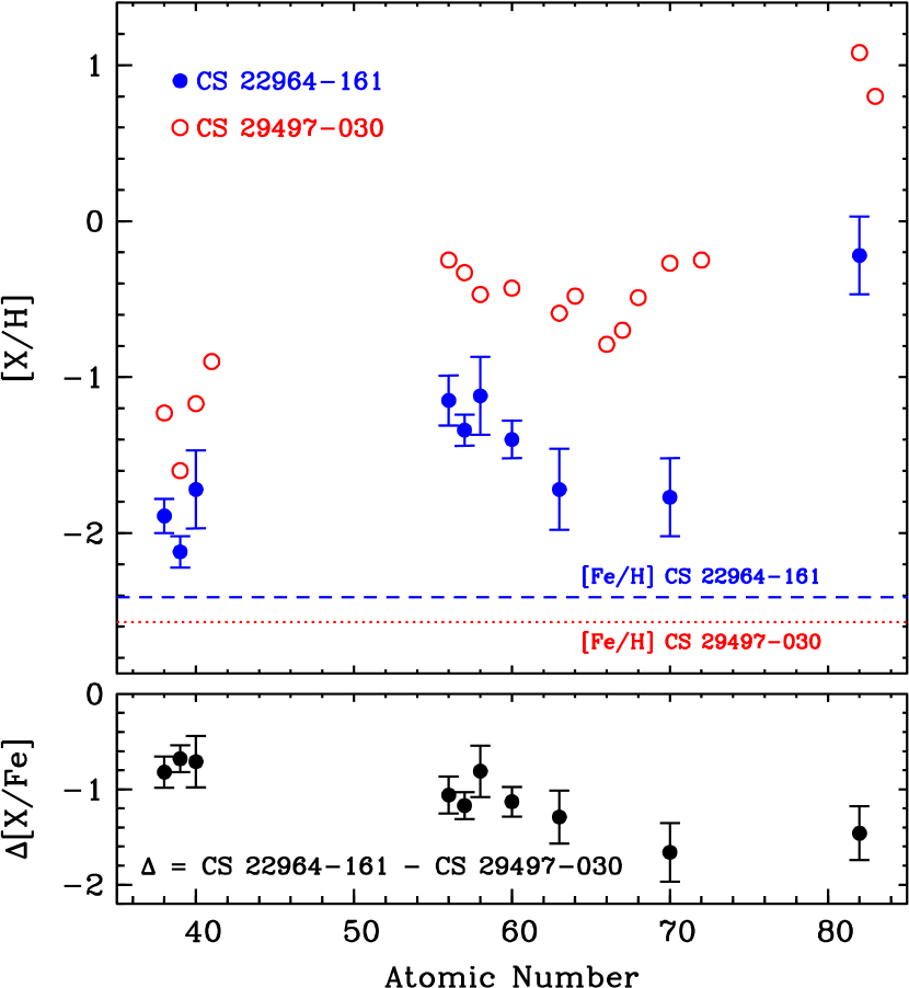
Figure 9: In the top panel, $n$-capture abundances relative to solar values [X/H] from the CS 22964-161 combined spectrum are plotted along with those of the BMP very $s$-process-rich star CS 29497-030 (Ivans et al. 2005). Horizontal lines are drawn to indicate the general Fe-metallicity levels of the two stars. In the bottom panel the abundance differences between these two stars are shown.

In the top panel of Figure 9 we plot the abundances relative to solar values for the 10 $n$-capture elements detected in the CS 22964-161 syzygy spectrum, together with the $n$-capture abundances in the very $s$-process-rich BMP star CS 29497-030. These two stars have nearly the same overall [Fe/H] metallicity, as indicated by the horizontal lines in the panel. The $n$-capture overabundance pattern of CS 22964-161 clearly identifies it as another member of C- and $s$-process-rich “lead star” family.

However, the relative $n$-capture abundance enhancements [X/Fe] of CS 29497-030 are about 1 dex higher than they are in CS 22964-161. This is emphasized by taking the difference between the two abundance sets, as is displayed in the lower panel of Figure 9. These differences illustrate the trend toward weaker $s$-process enhancements of the heaviest elements in CS 22964-161 compared to CS 29497-030.

Many studies have argued that these overall abundance anomalies, now seen in many low metallicity stars, must have originated from mass transfer from a (former) AGB companion to the stars observed today. Whole classes of stars with large C and $s$-process abundances are dominated by single-line spectroscopic binaries, including the high-metallicity “Ba II stars” (McClure, Fletcher, & Nemec 1980; McWilliam 1988; McClure & Woodsworth 1990), the low-metallicity red giant “CH stars” (McClure 1984), the “subgiant CH stars” (McClure 1997), and the BMP stars (Preston & Sneden 2000; note that not all BMP stars share these abundance characteristics). The case is especially strong for the subgiant CH and BMP stars, for these are much too unevolved to have synthesized C and $s$-process elements in their interiors and dredged these fusion products to the surfaces. Our analysis has confirmed that primary and secondary CS 22964-161 stars are on or near the main sequence. Therefore we suggest that a third, higher-mass star is now or once was a member of the CS 22964-161 system. During the AGB evolutionary phase of the third star, it transferred portions of its C- and $s$-process-rich envelope to the stars we now observe.

The very large Pb abundance of CS 22964-161 strengthens the AGB nucleosynthesis argument. Gallino et al. (1998) and Travaglio et al. (2001) predicted substantial Pb production in $s$-process fusion zones of metal-poor AGB stars. In metal-poor stars, the neutron-to-seed ratio is quite high, permitting the neutron-capture process to run through to Pb and Bi, the heaviest stable elements along the $s$-process path. Prior to this theoretical prediction, it was assumed that a $strong$ component of the $s$-process was required for the manufacture of half of the ²⁰⁸Pb in the solar system (Clayton & Rassbach 1967). That the patterns of the abundances of the neutron-capture elements in CS 22964-161 and CS 29497-030 resemble each other so well is a reflection of how easily low-metallicity AGB stars can synthesize the heavy elements.

8.1 Inferred Nucleosynthetic and Dilution History

We explored the origin of the neutron-capture enhancements in CS 22964-161 by comparing the derived photospheric abundances with predicted stellar yields from the $s$-process. Employing FRANEC stellar evolutionary computations (see Straniero et al. 2003; Straniero, Gallino, & Cristallo 2006), we performed nucleosynthetic calculations following those of Gallino et al.  (1998; 2006a) and Bisterzo et al. (2006). We then sought out good matches between the observed and predicted abundance pattern distributions with low-mass AGB progenitors of comparable metallicities and a range of initial masses.

We employed AGB models adopting different ¹³C-pocket efficiencies and initial masses to explore the nucleosynthetic history of the observed chemical compositions (Busso, Gallino & Wasserburg 1999; Straniero et al. 2003). Permitting some mixing of material between the $s$-process-rich contributions of the AGB donor, and the H-rich material of the atmosphere in which the contributions were deposited, we identified those AGB model progenitors that would yield acceptable fits for the predicted yields of all $s$-process elements beyond Sr.

Ascertaining the best matches between the observed and predicted yields was performed in the following way. For a given initial AGB mass, we inspected the abundances of [Zr/Fe], [La/Fe], and [Pb/Fe] for various ¹³C-pocket efficiencies adopted in the calculations. The difference between our predicted [La/Fe] and that of the observed abundance ratio gave us a first guess to the dilution of material for a given ¹³C-pocket efficiency. The dilution factor (dil) is defined as the logarithmic ratio of the mass of the envelope of the observed star polluted with AGB stellar winds and the AGB total mass transferred: dil $\equiv$ log$(M^{env}_{obs}/M^{AGB}_{transf})$. The ¹³C-pocket efficiency is defined in terms of the ¹³C pocket mass involved in an AGB pulse that was adopted by Gallino et al. (1998). Their §2.2 states, “The mass of the ¹³C pocket is 5.0$\times$10^-4 $M_{\odot}$ [here called ST], about 1/20 of the typical mass involved in a thermal pulse. It contains 2.8$\times$10^-6 $M_{\odot}$ of ¹³C.” Thus our shorthand notation for ¹³C-pocket efficiency will be ST/N, where ”N” is the reduction factor employed in generating a particular set of AGB abundance predictions. Subtracting this dilution amount from the predicted [Pb/Fe], we then compared the result to the observed [Pb/Fe]. The large range of ¹³C-pocket efficiencies was then narrowed down, keeping only those results that fit the abundances of both [La/Fe] and [Pb/Fe] within 0.2 dex. Similar iterations were performed employing the abundances of [Zr/Fe].

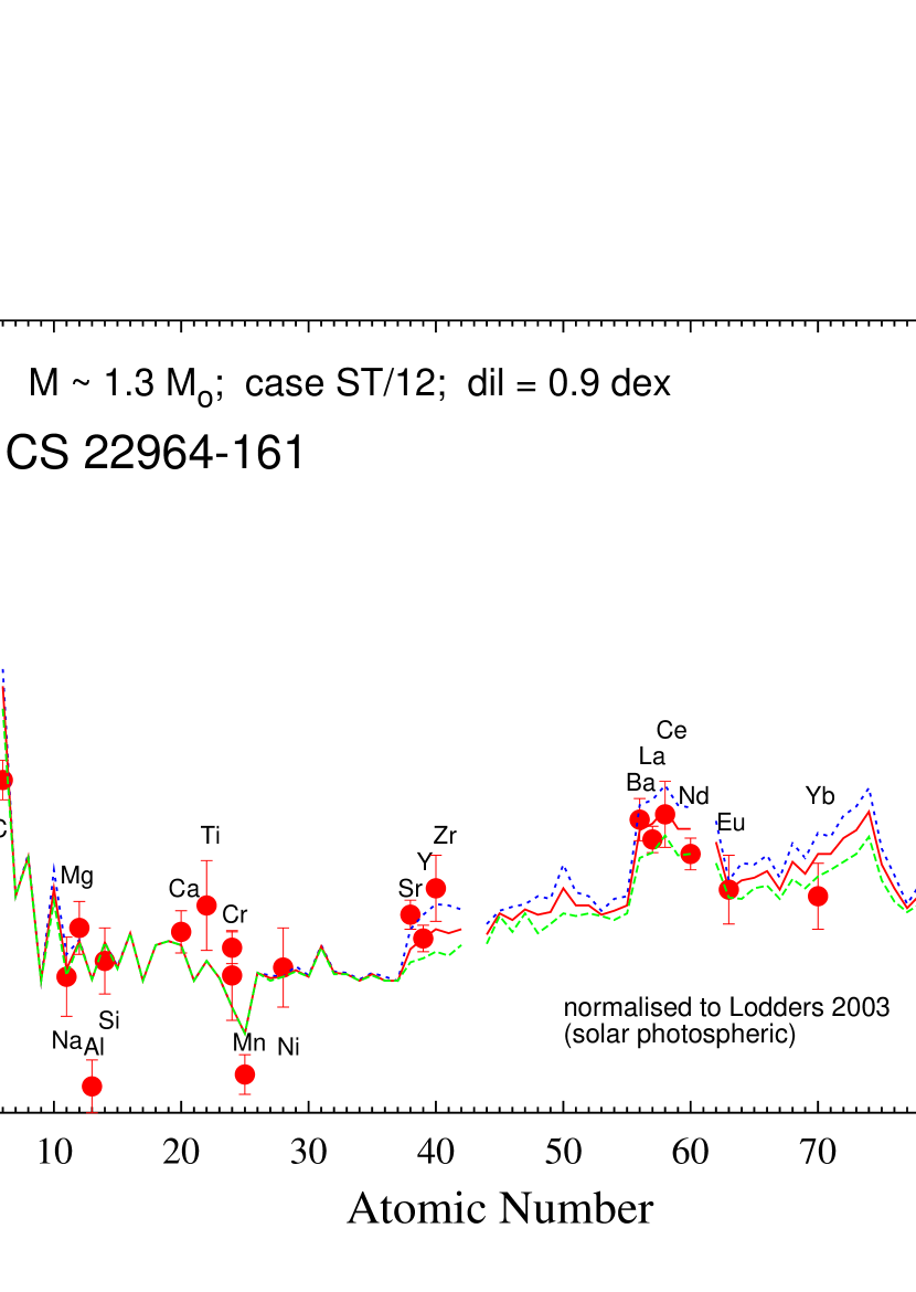
Figure 10: Comparison of the [X/Fe] abundances in CS 22964-161 with predictions from $s$-process calculations of a 1.3$M_{\odot}$ AGB star model. The solid red line corresponds to the best match between the observed and predicted abundance pattern. The dotted blue and dashed green lines indicate the difference that adopting models of $\pm$0.05$M_{\odot}$ would make (effectively, changing the number of thermal pulses from 4 to 6, identified in the figure legend as n4, n5, n6). For the specific choice of the ¹³C-pocket (ST/12), and for the definition of the dilution factor ($dil$), see the text.

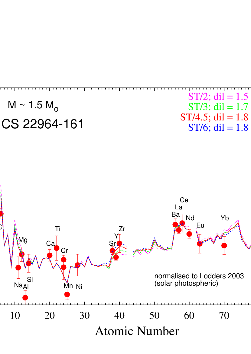
Figure 11: Comparison of the [X/Fe] abundances in CS 22964-161 with predictions from $s$-process calculations of a 1.5$M_{\odot}$ AGB star model. The solid red line corresponds to the best match between the observed and predicted abundance pattern. The dotted magenta, long-dashed green, and short-dashed blue lines show the difference made to the pattern by adopting different amounts of dilution. For discussion of the the various choices of the ¹³C-pocket efficiency (ST/N), and the dilution factor (dil), see the text.

We repeated this process for a range of initial AGB mass choices: 1.3, 1.5, 2, 3, and 5$M_{\odot}$. For AGB models of initial mass 3 and 5$M_{\odot}$ no good match was found because the light s-elements (ls $\equiv$ Sr, Y, Zr) were predicted to have too high abundances with respect to the heavy s-elements (hs $\equiv$ Ba, La, Ce, Nd). For AGB models of $M$ $\leq$ 2$M_{\odot}$ a satisfactory solution was found for ls, hs, and Pb, provided a proper ¹³C-pocket efficiency and dilution factor were chosen. In Figures 10 and 11 we show the matches between predicted and observed abundances for the two lowest-mass models, 1.3 and 1.5$M_{\odot}$, respectively.

The abundances of the light elements Na and Mg further narrowed the range of allowable AGB progenitor models. Two independent channels are responsible for creating ²³Na: the ²²Ne($p$,$\gamma$)²³Na reaction during H-shell burning, and the neutron capture on ²²Ne via the chain ²²Ne($n$,$\gamma$)²³Ne($\beta^{-}$$\nu$)²³Na in the convective He flash (see Mowlavi 1999; Gallino et al. 2006). A large abundance of primary ²²Ne derives from the primary ¹²C mixed with the envelope by previous third dredge up episodes, then converted to primary ¹⁴N by HCNO burning in the H-burning shell and followed by double $\alpha$ capture via the chain ¹⁴N($\alpha$,$\gamma$)¹⁸F($\beta^{+}$$\nu$)¹⁸O($\alpha$,$\gamma$)²²Ne during the early development of the convective thermal pulse. The next third dredge up episode mixes part of this primary ²²Ne with the envelope. Finally, while the H-burning shell advances in mass, all the ²²Ne present in the H shell is converted to ²³Na by proton capture, accumulating in the upper region of He intershell. Note that in intermediate mass AGB stars suffering the so-called hot bottom burning (HBB) in the deeper layers of their convective envelope, efficient production of ²³Na results from proton capture on ²²Ne (Karakas & Lattanzio 2003). Furthermore, the marginal activation in the convective He flash of the reactions ²²Ne($\alpha$,$n$)²⁵Mg and ²²Ne($\alpha$,$\gamma$)²⁶Mg would lead to enhanced Mg. At the same time, most neutrons released by ²²Ne($\alpha$,$n$)²⁵Mg are captured by the very abundant primary ²²Ne, thus producing ²³Na through the second channel indicated above.

Comparison of the abundance data in Figures 10 and 11 shows that the observed [Na/Fe] argues for the exclusion of the 1.5$M_{\odot}$ AGB model, which over-predicts this abundance ratio by $\sim$0.5 dex. The same statement applies to the 2$M_{\odot}$ model, not illustrated here. The larger Na abundances produced in these models, relative to the 1.3$M_{\odot}$ model, is related to the larger number of thermal pulses (followed by third dredge up) that these stars experience. These arguments leave the 1.3$M_{\odot}$ AGB model as the only one capable of providing a global good match to all observed elements.

In order to match these abundances, the predicted AGB yields require an inferred dilution by H-rich material. We do not know the distance between the AGB primary donor and the low mass companion (actually, the binary system) that is now observed. And, neither do we know precisely the mass loss rate of the AGB. Dilution by about 1 dex of $s$-process-rich AGB material with the original composition of the observed star, as we deduce on the basis of the above nucleosynthesis analysis, only fixes the ratio of the accreted matter with the outer envelope of the observed star. A more detailed discussion is taken up in §8.2.

A final remark concerns C, for which Figures 10 and 11 indicate an $\sim$0.8 dex over-production compared to the observed [C/Fe]. This mismatch can in principle be substantially reduced by the occurrence of the so-called cool bottom process (CBB: see Nollett, Busso, & Wasserburg 2003; Domínguez et al. 2004a,b). This reduction would imply a substantial increase of predicted N abundance, from [N/Fe] $\sim$ +0.5 shown in Figures 10 and 11 to perhaps +1.5. We attempted without success to detect the strongest CN absorption at the 3883 Å bandhead. Trial spectral syntheses of this wavelength region suggested that even [N/Fe] $\sim$ +1.5 would not produce detectable CN.

8.2 Mixing and Dilution in the Stellar Outer Layers

Very recently Stancliffe et al. (2007), extending the earlier discussion of Theuns, Boffin, & Jorissen (1996), report that extensive mixing due to thermohaline instability in a metal-poor star on the main sequence may severely dilute material that has been accreted from a companion. They computed the mixing time scale with the assumption that thermohaline convection behaved as a simple diffusion process, and they concluded that the new matter should rapidly be mixed down over about 90% of the stellar mass.

Treating thermohaline convection simply as diffusion does not take into account the special nature of this process, which has extensively been studied in oceanography (e.g. Veronis 1965; Kato 1966; Turner 1973; Turner & Veronis 2000; Gargett & Ruddick 2003), and has also been considered in stars (Gough & Toomre 1982, Vauclair 2004). Thermohaline convection occurs in the ocean when warm salty water comes on top of cool fresh water. In this case the stabilizing thermal gradient acts against the destabilizing salt gradient. If the stabilizing effect compensates the destabilizing one, the medium should be stable, but it remains unstable due to double-diffusion: when a blob begins to fall down, heat diffuses out of it more rapidly than salt; then the blob goes on falling as the two effects no longer compensate. This creates the well known “salt fingers”, thus is a very different physical environment than ordinary convection.

A similar situation occurs in stars when high-$\mu$ matter comes upon a lower-$\mu$ region, which is the case for hydrogen-poor accretion. This has been studied in detail for the case of planetary accretion on solar-type stars (Vauclair 2004). As shown in laboratory experiments (Gargett & Ruddick 2003) the fingers develop in a special layer with a depth related to the velocity of the blobs and to the dissipation induced by hydrodynamical instabilities at their edges. This is a complicated process which may also be perturbed by other competing hydrodynamical effects. Depending on the situation, it is possible that the “finger” regime stops before complete mixing of the high-$\mu$ material into the low-$\mu$ one. In this case, we expect that the final amount of matter that remains in the thin sub-photospheric convective zone depends only on the final $\mu$-gradient, whatever the original amount accreted: more accreted matter leads to more mixing so that the final result is the same.

Another very important point has to be mentioned. At the epoch when accretion occurs on the dwarfs, these stars are already about 3 to 4 Gyr old. Gravitational settling of helium and heavy elements has already occurred and created a stabilizing $\mu$-gradient below the convective zone (Vauclair 1999; Richard, Michaud, & Richer 2002). For example, as we illustrate in Figure 12, in a 0.78$M_{\odot}$ star with [Fe/H] = $-$2.3, after 3.75 Gyr the $\mu$-value is as low as 0.58 inside the convective zone while it goes up to nearly 0.60 in deeper layers. Thus the stabilizing $\Delta\mu/\mu$ is already of order 0.02. If the star accretes hydrogen-poor matter, thermohaline convection may begin but it remains confined by the $\mu$-barrier. The star can accrete as much high-$\mu$ matter as possible until this stabilizing $\mu$-gradient is flattened.

In §8.1 we saw, from the observed abundances and the AGB nucleosynthetic computations, that the dilution factor is of the order of 1 dex for the AGB model of initial mass $\sim$1.3$M_{\odot}$. Table 7 lists the predicted mass fraction of hydrogen ($X$), helium ($Y$), and heavier elements ($Z$) in the envelope of AGB progenitor stars of 1.3 and 1.5$M_{\odot}$ for two cases. The first case describes the final abundance mix produced by the AGB at the end of its nucleosynthetic lifetime (the last Third Dredge-Up). The second case describes the mass average of the winds from the AGB over its $s$-processing lifetime. Also noted is the mean molecular weight of the material ($\mu$), assuming fully ionized conditions. From Table 7, the $\mu$-value in the wind lies in the range 0.61 to 0.78. From these computations, we find that, after dilution, the $\mu$-value inside the convective zone should increase by $\Delta\mu/\mu\simeq 0.1\%$ to $4\%$. Clearly most of the inferred values for the dilution factor are compatible with stellar physics. For the lowest values it is possible that the accreted matter simply compensates the effect of gravitational diffusion. For larger values, thermohaline convection can have larger effects but, following Vauclair (2004), if we accept an inverse $\mu$-gradient of order $\Delta\mu/\mu$ = 0.02 below the convective zone, such an accreted amount would still be possible.

8.3 The Extraordinary Abundance of Lithium

Near main-sequence-turnoff CEMP stars display a variety of Li abundances. The majority have undetectable 6708 Å Li I lines, implying log $\epsilon$(Li) $<$ +1. A few have abundances similar to the Spite & Spite (1982) “plateau”: log $\epsilon$(Li) = +2.10 $\pm$ 0.09 (Bonifacio et al. 2007). These include our CEMP binary CS 22964-161, and at least CS 22898-027 (Thorburn & Beers 1992) and LP 706-7 (Norris, Ryan, & Beers 1997). A few more stars have Li abundances somewhat less than the Spite plateau value, e.g., log $\epsilon$(Li) $\simeq$ +1.7 in CS 31080-095 and CS 29528-041 (Sivarani et al. 2006). This CEMP Li abundance variety stands in sharp contrast to the nearly constant value exhibited by almost all normal metal-poor stars near the main-sequence turnoff region.

Although CS 22964-161 has a Spite plateau Li abundance, it is unlikely this is the same Li with which the system was born. Considering just the primary star, suppose that the C and $s$-process-rich material that it received was Li-free. If this material simply blanketed the surface of the primary, mixing only with the original Li-rich atmosphere and outer envelope skin, then the resulting observed Li would be at least less than the plateau value. Alternatively, if the transferred material induced more significant mixing of the stellar envelope, the surface Li would be severely diluted below the limit of detectability in the primary’s atmosphere. In order to produce the large observed Li abundance in the primary, freshly minted Li must have been transferred from the AGB donor star.

Li can be produced during the AGB phase both in massive AGB stars and in low-mass AGB stars via ³He($\alpha$,$\gamma$)⁷Be($e^{-},\nu_{e}$)⁷Li, but hot protons rapidly destroy it via ⁷Li($p$,$\alpha$)⁴He. Cameron & Fowler 1971) proposed that in some circumstances the freshly minted ⁷Be can however be transported to cooler interior regions before decaying to ⁷Li. In massive AGB stars ( 4$M_{\odot}$ $\lesssim$ $M$ $\lesssim$ 7$M_{\odot}$) nucleosynthesis at the base of the convective envelope (“hot bottom burning”; Scalo, Despain, & Ulrich 1975) can produce abundances via the Cameron-Fowler mechanism as high as log $\epsilon$(⁷Li) $\sim$ 4.5 (Sackmann & Boothroyd 1992). However, the lifetimes of these massive AGB stars are far too short to be considered as a likely source of Li in CS 22964-161.

In models of low-mass AGB stars (1$M_{\odot}$ $\leq$ $M$ $\leq$ 3$M_{\odot}$) of [Fe/H] = $-$2.7, Iwamoto et al. (2004) find that a H-flash episode can occur subsequent the first fully developed He shell flash. The convection produced by the He shell flash in this metal-poor star model can reach the bottom of the over-lying H-layer and bring protons down into the He intershell region, a region hot enough to induce a H flash. The high-temperature conditions of the H-flash can then produce ⁷Li by the Cameron-Fowler mechanism. Although the Iwamoto et al. 2.5$M_{\odot}$ model produced a weak H flash, the less massive models produced more energetic ones. In the lowest mass models, surface abundances of log $\epsilon$(⁷Li) $>$ 3.2 were achieved. Note that there is a maximum metallicity close to [Fe/H] = $-$2.5 beyond which such an H-flash is not effective at producing ⁷Li. Another viable mechanism for producing a very high abundance of ⁷Li in low mass AGB stars of higher metallicities, as observed in the intrinsic C(N) star Draco 461 ([Fe/H] = $-$2.0 $\pm$ 0.2), was advanced by Domínguez (2004a,b) and is based on the operation of the CBP introduced in §8.1.

Although $s$-process calculations were not performed in the Iwamoto et al. study, we note that it would seem that the parameters of the best-fit model of §8.1 would produce sufficient Li to fit the observations of CS 22964-161.

9 IMPLICATIONS FOR THE PUTATIVE AGB DONOR STAR

The binary nature of CS 22964-161 presents a unique opportunity to explore the nature of the AGB star presumably responsible for its abundance anomalies. The ingredients of the exploration are: (a) the analysis of our radial velocities of CS 22964-161 obtained over an interval of about 1100 days, (b) estimation of the orbit changes caused by accretion from an AGB companion, (c) stability of the hierarchical triple system in its initial and final states (Donnison & Mikulskis 1992, hereafter DM92; Szebehely & Zare 1977; Tokovinin 1997; Kiseleva, Eggleton, & Anolova 1994), and (d) application of an appropriate initial-final mass relation for stars of intermediate mass (Weidemann 2000, and references therein).

9.1 Evidence for an AGB relic?

Velocity residuals calculated for our orbit solution show no trend with time over the nearly 1100-day interval of observation. This is illustrated by the plot of orbital velocity residuals versus Julian Date in Figure 13. Thus, we have yet to find evidence for a third component in the system. The Julian Date interval of our CS 22964-161 data is modest compared to the longest orbital periods of the so-called Barium and CH giant stars (McClure & Woodsworth 1990) and main-sequence/subgiant CH stars (McClure 1997) summarized in Table 6. On the other hand the errors of our observations ($\sigma$ = 0.5 km s^-1) are small compared to typical velocity semi-amplitudes of these comparison C-rich stellar samples, so drift of the center-of-mass velocity by as much as 1 km s^-1 due to the presence of a third star should be detectable. Accordingly, Figure 13 encourages us to contemplate the possibility that CS 22964-161 is not accompanied by a white dwarf relic of AGB evolution. Continuing observation will be required to test this notion.

9.2 Change in Orbit Dimensions Induced by Accretion

The consequences of mass accretion by a binary were first explored by Huang (1956), who calculated the change in semi-major axis of a binary embedded in a stationary interstellar cloud. Using McCrea’s (1953) “retarding force” that followed from Bondi-Hoyle-Lyttleton accretion theory (Bondi & Hoyle 1944), Huang found that mass accretion shrinks orbits, and he proposed that this process could produce close binaries. The problem of binary accretion has been revisited in recent years by numerical simulations of star formation in molecular clouds. Bate & Bonnell (1997) calculate the changes in binary separation due to accretion by an infalling circumstellar cloud. The change is very sensitive to the assumed specific angular momentum (SAM) carried by the accreted material. In the case of low SAM they recover Huang’s result. For large SAM orbits the binaries expand. More recently Soker (2004) has calculated the SAM of mass accreted by a binary system embedded in the wind of an AGB star, which is our case. For triple systems containing a distant AGB companion with approximately coplanar inner and outer orbital orbits (statistically most probable in the absence of a special orientation mechanism) he also recovers Huang’s result. Finally, building on an earlier analysis by Davies & Pringle (1980), Livio et al. (1986) found that the rate of accretion of angular momentum from winds is significantly less than that deposited in the simple Bondi-Hoyle accretion model.

Our gloss on all these analyses is that the most likely consequence of mass transfer to CS 22964-161 from its AGB companion a long time ago was a decrease in separation, i.e., the initial separation was larger than its present value of $\sim$0.9 AU. Conservatively, we use 0.9 AU as a lower limit in the estimates that follow below.

Empirical stability criteria for hierarchical triple systems are expressed as the ratio of the semi-major axis of the outer orbit to the semi-major axis of inner orbit (Heintz 1978; Szebehely & Zare 1977), and alternatively as the ratio of periods of the outer and inner orbits (Kiseleva et al. 1994; Tokovinin 1997). If these ratios exceed critical values, a triple system can be long-lived. Note, however, the cautionary remarks of Szebehely & Zare about the role of component masses in evaluation of stability for particular cases, and the relevance of these masses to the conclusions of DM92 about the fate of our AGB relic.

Let $a_{12}$ be the semi-major axis of the relative orbit of CS 22964-161 and $a_{3}$ be the relative semi-major axis that joins the center of mass of CS 22964-161 to the 3^rd (AGB-to-be) star. If we accept the Heintz (1978) and Szebehely & Zare (1977) stability criterion $a_{3}/a_{12}$ $>$ 8, then $a_{3}$ $>$ 7.3 AU and the orbital period of the outer binary had to be $P$ $>$ 4000 d. For Tokovinin’s (1997) more permissive criterion, $P_{3}/P_{12}$ $>$ 10 the minimum period is $P$ $>$ 2500 d and $a_{3}/a_{12}$ $>$ 4.6. Under these conditions none of our candidate metal-poor AGB stars (see the discussion in §8.1) with $M$ $<$ 2$M_{\odot}$ fill the Roche lobes (Marigo & Girardi 2007) of these minimum orbits, so wind accretion must have been the mechanism of mass transfer. According to Theuns et al. (1996) a 3$M_{\odot}$ AGB star in a 3-AU circular orbit will transfer no more than $\sim$1% of its wind mass to a 1.5 solar mass companion by wind accretion. Applying their result to our case, $M$(AGB) $\leq$ 1.5$M_{\odot}$ and AGB relic mass $\sim$0.5$M_{\odot}$, the maximum mass transfer is about (1.5$-$0.5)$\times$0.015 $\simeq$ 0.015$M_{\odot}$.

The remainder of the AGB wind mass is ejected from the system. We calculated the change in period and semi-major axis of the AGB orbit following Hilditch (2001) for the case of a spherically symmetric wind. The orbit expands and the period lengthens according to

$${\rm ln}(a_{f}/a_{i})={\rm ln}(1+u_{i})-{\rm ln}(1+u_{f})$$

and

$${\rm ln}(P_{f}/P_{i})=2\times{\rm ln}(1+u_{i})-2\times{\rm ln}(1+u_{f})$$

in which initial and final values of $u$ are $u_{i}=M_{3i}/(M_{1}+M_{2})$ and $u_{f}=M_{3f}/(M_{1}+M_{2})$ . We have ignored small changes in $M_{1}$ and $M_{2}$. For $M_{3}$ = 1.3 $M_{\odot}$ and the Tokovinin (1997) stability condition ($a_{3}/a_{12}$ $>$ 4.6), the minimum orbit expands from 4.2 AU to 5.9 AU and the minimum period lengthens from 1900 days to 3700 days. For the more restrictive Heintz ($a_{3}/a_{12}$ $>$ 8) stability condition the minimum orbit expands from 7.3 AU to 10.2 AU and the minimum period lengthens from 4300 days to 8400 days. The K-values for the center-of-mass of the CS 22964-161 binary for the two cases are 4.3 km s^-1 and 3.3 km s^-1, respectively, both readily detectable by conventional echelle spectroscopy.

9.3 Dynamical Stability of CS 22964-161 as a Hierarchical Triple System

The DM92 study investigated the stability of triple systems that consist of a close inner binary with masses ($M_{1},M_{2}$) and semi-major axis $a1$ attended by a remote companion of mass $M_{3}$ at distance $q2$ from the center of mass of the inner binary. They use the parameter notation of Harrington’s (1975) pioneering numerical simulations. DM92 investigate stability in three mass regimes, by integration of the equations of motion for various sets of masses, initial positions and velocities:
                                  case (i): $M_{3}$ $\leq$ minimum($M_{1},M_{2}$)
                                  case (ii): $M_{1}$ $\geq$ $M_{3}$ $\geq$ $M_{2}$
                                  case (iii): $M_{3}$ $\geq$ maximum($M_{1},M_{2}$)
They pursued the integrations for at least 1000 orbits of the inner binary or until disruption, which ever happened first. Among the several results in §5 of their paper one is of particular interest for us: in their words “When $M_{3}$ was the least massive body in the system, the system invariably became unstable through the tendency of $M_{3}$ to escape from the system altogether.” Accepting the McClure (1984) paradigm, we suppose that CS 22964-161 began its existence as a case (iii) hierarchical triple system in which a relatively low-mass AGB progenitor (§8.1) was orbited by a close binary with component masses only slightly smaller than their present values, $M_{1}$sin${}^{3}i$ = 0.77$M_{\odot}$ and $M_{2}$sin${}^{3}i$ = 0.68 $M_{\odot}$. Evidently, the distance between $M_{3}$ and the close binary was large enough to insure stability during the lifetime of $M_{3}$. Curiously, although Kiseleva et al. (1994) made numerical simulations apparently similar to those of DM92, they make no mention of the ejection of low-mass outer components that attracted our attention to DM92.

We confine our attention to initial values of AGB mass $<$2.0$M_{\odot}$, adopted in accordance with the nucleosynthetic calculations in §8.1. In the late stages of AGB evolution the system evolved from case (iii) to case (i) via mass loss due to the AGB superwind. For all acceptable models in §8.1 the mass of the WD relic for an AGB initial mass model of 1.3$M_{\odot}$ is less than 0.60$M_{\odot}$ (Weidemann 2000). Therefore, according to DM92 $M_{3}$ will be ejected following this ancient AGB evolution. Our extant radial velocity data suggest that the ejection already occurred. From the effect of the AGB relic on the $\gamma$ velocity of CS 22964-161 calculated above we believe that this conclusion can be tested by future observations.

10 CONCLUSIONS

We have obtained high resolution, high S/N spectra over a three-year period for CS 22964-161, which was known to be metal-poor and C-rich from previous low resolution spectroscopic studies. We discovered CS 22964-161 to be a double-line spectroscopic binary, and have derived the binary orbital parameters ($P$ = 252 d, $e$ =0.66, $M_{p}~{}sin^{3}~{}i$ = 0.77 $M_{\odot}$, $M_{s}~{}sin^{3}~{}i$ = 0.68 $M_{\odot}$). Both binary members lie near the metal-poor main-sequence turnoff ($T_{\rm eff}$_,p = 6050 K, log g_p = 3.7, and $T_{\rm eff}$_,s =5850 K, log g_s = 4.1). We derived similar overall metallicities for primary and secondary, [Fe/H] = $-$2.4 and similar abundance ratios [X/Fe]. In particular, both stars are similarly enriched in C and the $n$-capture elements, with a clear $s$-process nucleosynthesis signature. The primary has a large Li content; the secondary’s Li I feature is undetectably weak, and does not usefully constrain its Li abundance.

The observed Li, C and $s$-process abundances of the CS 22964-161 system must have been produced by an AGB star whose relic, depending on its mass, may have been ejected from the post-AGB hierarchical triple. It seems AGB enrichment was produced by minor mass accretion in the AGB super-wind rather than Roche-lobe overflow. As discussed in §8, and contrary to the thermohaline diffusion suggestion of Stancliffe et al. (2007), such hydrogen-poor accreted matter probably remained in the outer stellar layers, owing to the stabilizing $\mu$-gradient induced by helium gravitational settling. Strong thermohaline diffusion is difficult to reconcile with the observed Li: about 9/10 of the stellar mass would be efficiently mixed on a time scale of 1 Gyr, which would imply the complete destruction of ⁷Li because of the very high temperature reached in the inner zones. It seems more likely that the moderate thermohaline mixing discussed §8, related to the effect of gravitational settling in the first 3 to 4 Gyr before mass accretion by the AGB donor, would save the Li from destruction. In the model of a low mass AGB of low metallicity calculated by Domínguez et al. (2004a,b) with the inclusion of “cool bottom processing” during the AGB phase, log $\epsilon$(Li) $>$ 3 is achieved in the envelope. A dilution factor of about 1 dex would bring the Li abundance into accord with the observed value.

Figure 1: Top panel: radial velocity observations of CS 22964-161 primary and secondary stars, and best-fit orbital solutions from these velocities. Circles represent data taken with MIKE on the Magellan Clay telescope and squares represent data taken with the echelle spectrograph on the du Pont telescope. Filled symbols represent data for the primary and open symbols are for the secondary. The lines are fits to the Magellan data only. Bottom panel: differences of the observed velocities and the orbital solutions.

Figure 2: Observed composite absorption spectra of primary and secondary stars. The bottom spectrum is the spectrum at syzygy ($\Delta V_{R}$ = 0 km s^-1); this is the mean of three individual observations. The middle spectrum is the mean of three observations obtained at phases with $\Delta V_{R}$ = 60 km s^-1. The top spectrum represents the original syzygy spectrum after application of a velocity shift of 60 km s^-1 and dilution by addition of a continuum flux that yields secondary line depths approximately matching those seen in the middle spectrum. Dotted lines point to secondary positions of a few lines that are very strong in the primary spectrum. The flux scale of the syzygy spectrum is correct, and that other two spectra have been vertically shifted in the figure for display purposes. The rest wavelength scale is that of the primary star.

Figure 3: Comparison of observed equivalent widths of the secondary star inferred from the syzygy spectrum and those measured directly from the six spectra with large velocity splits between primary and secondary stars. Measurements for each spectral feature are connected by vertical lines and labeled with the feature wavelength. Medians of the $EW$s are displayed as $\times$ symbols. The dashed slanting line indicates equality of $EW$ values.

Figure 4: Iron abundances plotted as a function of wavelength for primary (top panel) and secondary (bottom panel) stars. The symbols are defined in the figure legend. Dashed horizontal lines are drawn to indicate the mean Fe I abundances of primary and secondary stars, log $\epsilon$(Fe) = 5.13 and 5.11, respectively.

Figure 8: Selected spectral features of $n$-capture species in the CS 22964-161 syzygy spectrum.

Figure 12: Mean molecular weight ($\mu$) and temperature (T) profiles, as functions of the fractional mass (mass above the considered layer), in a 0.78$M_{\odot}$ star with [Fe/H] = –2.3, at an age of 3.75 Gyr. Here $\mu$ is the real molecular weight, including partial ionization. The fractional mass of the convective zone is 0.004. The helium depletion due to gravitational settling, of about 20% in this case, already leads to an important stabilizing $\mu$-gradient below the convective zone. This model is one of those computed by Richard et al. (2002), including pure atomic diffusion. The full model was made available to us by Richard (private communication).

Figure 13: Velocity residuals to the fitted orbit are plotted against the date of observation for the Magellan data. Filled circles represent the primary and open circles represent the secondary. These residuals show no trend with time.

Table 1: Velocity Measurements for CS22964-161

HJD	Vp	Vs	Phase
(- 2440000)	km s-1	km s-1
du Pont Observations
13592.52532	24.79	41.04	0.0716
13592.56468	24.63	42.35	0.0718
13593.52234	25.34	38.32	0.0756
13593.56091	25.21	40.26	0.0757
13867.92873	36.59	27.00	0.1623
13870.91114	36.44	25.90	0.1741
13871.85817	37.22	26.27	0.1778
Magellan Observations
13230.66465	38.43	25.01	0.6386
13580.79663	5.09	65.21	0.0252
13585.74591	14.80	52.79	0.0448
13587.62635	18.56	49.77	0.0522
13602.62780	32.29	$\cdots$	0.1116
13603.50474	33.00	$\cdots$	0.1151
13606.50536	33.83	$\cdots$	0.1270
13631.67197	39.08	26.29	0.2266
13634.54878	39.06	25.43	0.2380
13817.90625	6.10	64.19	0.9642
13832.88449	4.11	66.51	0.0235
13834.88836	8.21	60.76	0.0314
13889.88563	40.09	25.83	0.2492
13890.73000	40.19	26.24	0.2526
13891.72338	40.03	25.80	0.2565
13891.79617	39.87	25.63	0.2568
13891.91199	39.79	25.33	0.2572
13892.72313	40.47	25.77	0.2604
13892.91348	40.03	25.21	0.2612
13893.76837	40.02	25.34	0.2646
13897.80466	40.22	24.87	0.2806
13898.72511	40.00	24.35	0.2842
13917.74748	40.82	23.51	0.3595
13919.72723	40.20	23.00	0.3674
13935.76042	41.08	23.66	0.4309
13938.71168	41.14	23.29	0.4426
13938.73591	41.10	23.53	0.4427
13951.57253	40.34	23.09	0.4935
13989.60930	38.73	25.04	0.6441
13990.59320	38.69	25.36	0.6480
14197.85590	40.80	23.87	0.4689
14258.82674	37.60	28.04	0.7088
14259.78553	37.50	27.81	0.7126
14316.78097	15.19	52.81	0.9383
14317.65762	13.63	53.75	0.9418
14328.67079	-4.33	74.49	0.9854
14329.70221	-5.60	75.71	0.9895
14333.56647	-5.03	75.31	0.0048
14334.49082	-3.13	74.78	0.0085
14335.48607	-1.45	72.22	0.0124
14336.53932	0.46	69.88	0.0166

Table 2: Orbital Parameters for CS22964-161

Parameter	Value
$P$ (days)	252.481$\pm$0.043
$T_{0}$ (HJD-244 0000)	13827.383$\pm$0.103
$\gamma~{}(km~{}s^{-1})$	32.85$\pm$ 0.05
$K_{p}~{}(km~{}s^{-1})$	23.65$\pm$0.10
$K_{s}~{}(km~{}s^{-1})$	26.92$\pm$0.13
$e$	0.6564$\pm$0.0024
$\omega$ (deg)	188.54$\pm$0.39
$\sigma_{p}~{}(km~{}s^{-1})$	0.37
$\sigma_{s}~{}(km~{}s^{-1})$	0.56
Derived quantities:
$A~{}sin~{}i$ ($R_{\odot}$)	190.32$\pm$0.65
$M_{p}~{}sin^{3}~{}i$ ($M_{\odot}$)	0.773$\pm$0.009
$M_{s}~{}sin^{3}~{}i~{}$($M_{\odot}$)	0.680$\pm$0.007

Table 3: Line List for CS 22964$-$161

Species	$\lambda$	$\chi$	log $gf$	$EW_{p,o}$	$EW_{p,t}$	$EW_{s,o}$	$EW_{s,t}$
	Å	eV		mÅ	mÅ	mÅ	mÅ
Li I	6707.80	0.00	$+$0.18	24	29	$\cdots$	$\cdots$
Mg I	3829.36	2.71	$-$0.21	104	122	31	222
Mg I	3832.31	2.71	$+$0.14	128	150	30	213
Mg I	4703.00	4.35	$-$0.38	40	47	8	55
Mg I	5172.70	2.71	$-$0.38	127	152	25	156
Mg I	5183.62	2.72	$-$0.16	144	172	28	174
Mg I	5528.42	4.35	$-$0.34	40	49	10	63
Al I	3961.53	0.01	$-$0.34	62	73	11	79
Si I	3905.53	1.91	$+$0.09	$\cdots$	$\cdots$	$\cdots$	$\cdots$
Ca I	4226.74	0.00	$+$0.24	134	158	27	180
Ca I	5349.47	2.71	$-$0.31	11	13	$\cdots$	$\cdots$
Ca I	5588.76	2.53	$+$0.36	21	28	3	27
Ca I	5857.46	2.93	$+$0.24	17	21	$\cdots$	$\cdots$
Ca I	6102.73	1.88	$-$0.79	12	14	4	23
Ca I	6122.23	1.89	$-$0.32	26	33	2	12
Ca I	6162.18	1.90	$-$0.09	33	41	4	27
Ca I	6439.08	2.52	$+$0.39	28	36	3	22
Sc II	3645.31	0.02	$-$0.42	43	50	8	61
Sc II	4246.84	0.31	$+$0.24	59	69	8	55
Ti II	3477.19	0.12	$-$1.06	85	99	$\cdots$	$\cdots$
Ti II	3510.85	1.89	$+$0.14	55	64	$\cdots$	$\cdots$
Ti II	3596.05	0.61	$-$1.22	43	50	12	90
Ti II	3641.34	1.24	$-$0.71	40	46	12	86
Ti II	3759.30	0.61	$+$0.20	97	113	19	137
Ti II	4394.06	1.22	$-$1.77	16	18	$\cdots$	$\cdots$
Ti II	4443.80	1.08	$-$0.70	55	66	6	45
Ti II	4444.56	1.12	$-$2.21	14	16	$\cdots$	$\cdots$
Ti II	4468.49	1.13	$-$0.60	59	71	7	52
Ti II	4501.27	1.12	$-$0.76	54	65	5	40
Ti II	5336.79	1.58	$-$1.63	13	16	$\cdots$	$\cdots$
Cr I	3578.69	0.00	$+$0.41	59	69	13	97
Cr I	3593.50	0.00	$+$0.31	65	76	6	46
Cr I	4254.33	0.00	$-$0.11	57	67	4	29
Cr I	4274.80	0.00	$-$0.23	72	84	$\cdots$	$\cdots$
Cr I	4289.72	0.00	$-$0.36	63	74	7	44
Cr I	4646.17	1.03	$-$0.73	5	6	2	14
Cr I	5206.04	0.94	$+$0.03	29	35	6	36
Cr I	5409.79	1.03	$-$0.71	15	18	$\cdots$	$\cdots$
Cr II	4558.65	4.07	$-$0.66	8	9	2	10
Cr II	4588.20	4.07	$-$0.64	6	7	$\cdots$	$\cdots$
Mn I	4030.76	0.00	$-$0.48	$\cdots$	$\cdots$	$\cdots$	$\cdots$
Mn I	4033.06	0.00	$-$0.62	$\cdots$	$\cdots$	$\cdots$	$\cdots$
Mn I	4034.49	0.00	$-$0.81	$\cdots$	$\cdots$	$\cdots$	$\cdots$
Fe I	3475.46	0.09	$-$1.05	82	94	34	249
Fe I	3476.71	0.12	$-$1.51	73	84	8	61
Fe I	3490.59	0.05	$-$1.11	76	88	16	117
Fe I	3497.84	0.11	$-$1.55	71	82	8	58
Fe I	3521.27	0.91	$-$0.99	56	65	15	111
Fe I	3554.94	2.83	$+$0.54	47	55	6	45
Fe I	3558.53	0.99	$-$0.63	68	79	16	113
Fe I	3565.40	0.96	$-$0.13	89	103	21	151
Fe I	3570.13	0.91	$+$0.18	151	175	26	190
Fe I	3581.21	0.86	$+$0.42	114	132	36	262
Fe I	3606.69	2.69	$+$0.32	41	47	8	59
Fe I	3608.87	1.01	$-$0.09	80	92	20	142
Fe I	3618.78	0.99	$+$0.00	88	102	30	219
Fe I	3631.48	0.96	$+$0.00	102	118	23	168
Fe I	3647.85	0.91	$-$0.14	82	95	22	162
Fe I	3679.92	0.00	$-$1.58	69	80	17	125
Fe I	3687.47	0.86	$-$0.80	87	102	11	77
Fe I	3727.63	0.96	$-$0.61	83	96	10	75
Fe I	3745.57	0.09	$-$0.77	100	116	25	176
Fe I	3745.91	0.12	$-$1.34	89	104	10	72
Fe I	3758.24	0.96	$-$0.01	100	116	21	149
Fe I	3763.80	0.99	$-$0.22	86	99	15	106
Fe I	3787.89	1.01	$-$0.84	69	80	10	71
Fe I	3820.44	0.86	$+$0.16	114	133	22	157
Fe I	3825.89	0.92	$-$0.02	99	116	22	153
Fe I	3840.45	0.99	$-$0.50	74	87	20	140
Fe I	3856.38	0.05	$-$1.28	84	98	11	76
Fe I	3865.53	1.01	$-$0.95	67	79	11	76
Fe I	3899.72	0.09	$-$1.51	70	81	19	135
Fe I	3917.18	0.99	$-$2.15	27	31	4	27
Fe I	3922.92	0.05	$-$1.63	75	87	16	110
Fe I	3949.96	2.18	$-$1.25	18	21	6	38
Fe I	4005.25	1.56	$-$0.58	61	71	12	85
Fe I	4071.75	1.61	$-$0.01	79	92	17	125
Fe I	4134.69	2.83	$-$0.65	19	22	4	29
Fe I	4143.88	1.56	$-$0.51	68	80	8	53
Fe I	4147.68	1.49	$-$2.07	12	14	4	29
Fe I	4175.64	2.85	$-$0.83	18	21	$\cdots$	$\cdots$
Fe I	4187.05	2.45	$-$0.51	38	45	2	16
Fe I	4187.81	2.42	$-$0.51	42	49	6	41
Fe I	4191.44	2.47	$-$0.67	26	30	8	54
Fe I	4199.10	3.05	$+$0.16	52	61	$\cdots$	$\cdots$
Fe I	4202.04	1.49	$-$0.69	62	72	13	85
Fe I	4216.19	0.00	$-$3.36	24	28	2	13
Fe I	4222.22	2.45	$-$0.91	24	28	$\cdots$	$\cdots$
Fe I	4233.61	2.48	$-$0.58	37	43	4	24
Fe I	4250.13	2.47	$-$0.38	47	56	$\cdots$	$\cdots$
Fe I	4260.48	2.40	$+$0.08	61	72	10	69
Fe I	4271.16	2.45	$-$0.34	58	69	20	131
Fe I	4271.77	1.49	$-$0.17	93	109	11	77
Fe I	4282.40	2.18	$-$0.78	34	39	8	52
Fe I	4383.55	1.48	$+$0.21	104	122	15	100
Fe I	4404.75	1.56	$-$0.15	76	90	14	92
Fe I	4415.12	1.61	$-$0.62	62	73	16	108
Fe I	4427.32	0.05	$-$2.92	37	44	10	65
Fe I	4430.61	2.22	$-$1.73	10	12	2	15
Fe I	4447.72	2.22	$-$1.34	19	22	4	27
Fe I	4461.65	0.09	$-$3.19	20	24	8	52
Fe I	4466.55	2.83	$-$0.60	19	22	9	59
Fe I	4489.73	0.12	$-$3.90	6	6	3	20
Fe I	4494.56	2.20	$-$1.14	23	27	3	20
Fe I	4528.61	2.18	$-$0.89	35	42	8	51
Fe I	4602.95	1.49	$-$2.21	13	15	2	16
Fe I	4871.32	2.87	$-$0.36	25	29	5	34
Fe I	4872.14	2.88	$-$0.57	25	30	$\cdots$	$\cdots$
Fe I	4890.76	2.88	$-$0.39	24	29	10	65
Fe I	4891.50	2.85	$-$0.11	37	44	8	49
Fe I	4903.32	2.88	$-$0.93	12	14	$\cdots$	$\cdots$
Fe I	4919.00	2.87	$-$0.34	29	34	6	35
Fe I	5006.12	2.83	$-$0.61	23	28	$\cdots$	$\cdots$
Fe I	5014.94	3.94	$-$0.27	12	15	4	22
Fe I	5049.83	2.28	$-$1.35	18	21	8	49
Fe I	5133.69	4.18	$+$0.20	11	13	7	45
Fe I	5191.47	3.04	$-$0.55	21	25	$\cdots$	$\cdots$
Fe I	5192.35	3.00	$-$0.42	30	36	$\cdots$	$\cdots$
Fe I	5194.95	1.56	$-$2.02	17	25	$\cdots$	$\cdots$
Fe I	5202.34	2.18	$-$1.84	11	13	$\cdots$	$\cdots$
Fe I	5216.28	1.61	$-$2.08	16	19	$\cdots$	$\cdots$
Fe I	5232.95	2.94	$-$0.06	39	48	3	29
Fe I	5266.56	3.00	$-$0.39	24	29	4	21
Fe I	5269.55	0.86	$-$1.33	70	86	15	98
Fe I	5283.63	3.24	$-$0.52	17	20	3	20
Fe I	5324.19	3.21	$-$0.10	25	30	$\cdots$	$\cdots$
Fe I	5328.05	0.92	$-$1.47	68	81	13	82
Fe I	5371.50	0.96	$-$1.64	55	66	12	77
Fe I	5383.38	4.31	$+$0.65	17	20	$\cdots$	$\cdots$
Fe I	5397.14	0.92	$-$1.98	47	56	5	32
Fe I	5405.78	0.99	$-$1.85	44	52	9	61
Fe I	5429.71	0.96	$-$1.88	46	56	10	59
Fe I	5434.53	1.01	$-$2.13	36	44	7	40
Fe I	5446.92	0.99	$-$1.91	39	49	20	106
Fe I	5501.48	0.96	$-$3.05	10	12	$\cdots$	$\cdots$
Fe I	5506.79	0.99	$-$2.79	15	18	5	29
Fe I	5569.63	3.42	$-$0.50	11	14	3	17
Fe I	5572.85	3.40	$-$0.28	15	19	$\cdots$	$\cdots$
Fe I	5586.77	3.37	$-$0.10	21	25	5	30
Fe I	5615.66	3.33	$+$0.05	24	28	5	27
Fe I	6136.62	2.45	$-$1.41	16	19	$\cdots$	$\cdots$
Fe I	6191.57	2.43	$-$1.42	13	16	$\cdots$	$\cdots$
Fe I	6230.74	2.56	$-$1.28	16	19	3	17
Fe I	6393.61	2.43	$-$1.58	13	16	$\cdots$	$\cdots$
Fe I	6400.01	3.60	$-$0.29	13	16	$\cdots$	$\cdots$
Fe I	6430.85	2.18	$-$1.95	10	12	$\cdots$	$\cdots$
Fe I	6494.98	2.40	$-$1.24	22	26	12	66
Fe II	4178.86	2.57	$-$2.48	20	23	$\cdots$	$\cdots$
Fe II	4233.17	2.58	$-$2.00	37	44	3	19
Fe II	4508.28	2.84	$-$2.22	16	19	$\cdots$	$\cdots$
Fe II	4555.89	2.82	$-$2.28	12	14	5	33
Fe II	4923.92	2.89	$-$1.32	48	56	8	47
Fe II	5234.62	3.22	$-$2.05	17	20	$\cdots$	$\cdots$
Fe II	5275.99	3.20	$-$1.94	15	18	$\cdots$	$\cdots$
Co I	3502.29	0.43	$+$0.07	52	61	11	81
Co I	3506.33	0.51	$-$0.04	39	46	9	65
Ni I	3472.56	0.11	$-$0.82	55	64	11	79
Ni I	3483.78	0.27	$-$1.12	50	57	$\cdots$	$\cdots$
Ni I	3500.86	0.17	$-$1.37	54	62	12	89
Ni I	3510.33	0.21	$-$0.65	73	84	12	90
Ni I	3515.07	0.11	$-$0.26	70	81	17	124
Ni I	3519.76	0.27	$-$1.42	36	41	5	37
Ni I	3524.54	0.03	$-$0.03	84	97	16	118
Ni I	3566.39	0.42	$-$0.27	64	74	12	84
Ni I	3597.71	0.21	$-$1.09	44	51	12	87
Ni I	3619.40	0.42	$-$0.04	82	95	7	50
Sr II	4077.71	0.00	$+$0.17	(86)	(101)	(16)	(110)
Sr II	4215.52	0.00	$-$0.17	(80)	(94)	(15)	(99)
Y II	3611.04	0.13	$+$0.01	$\cdots$	$\cdots$	$\cdots$	$\cdots$
Y II	3710.29	0.18	$+$0.46	$\cdots$	$\cdots$	$\cdots$	$\cdots$
Y II	3774.33	0.13	$+$0.21	$\cdots$	$\cdots$	$\cdots$	$\cdots$
Zr II	4208.99	0.71	$-$0.46	$\cdots$	$\cdots$	$\cdots$	$\cdots$
Ba II	4554.03	0.00	$+$0.17	(92)	(108)	(13)	(82)
Ba II	4934.10	0.00	$-$0.16	(82)	(98)	(10)	(62)
Ba II	5853.69	0.60	$-$0.91	$\cdots$	$\cdots$	$\cdots$	$\cdots$
Ba II	6141.73	0.70	$-$0.08	(58)	(71)	(8)	(46)
Ba II	6496.91	0.60	$-$0.38	(53)	(65)	(7)	(36)
La II	3988.51	0.17	$+$0.21	$\cdots$	$\cdots$	$\cdots$	$\cdots$
La II	3995.74	0.17	$-$0.06	$\cdots$	$\cdots$	$\cdots$	$\cdots$
La II	4086.71	0.00	$-$0.07	$\cdots$	$\cdots$	$\cdots$	$\cdots$
La II	4123.22	0.32	$+$0.13	$\cdots$	$\cdots$	$\cdots$	$\cdots$
Ce II	4137.65	0.52	$+$0.44	$\cdots$	$\cdots$	$\cdots$	$\cdots$
Nd II	4021.33	0.32	$-$0.10	$\cdots$	$\cdots$	$\cdots$	$\cdots$
Nd II	4061.08	0.47	$+$0.55	$\cdots$	$\cdots$	$\cdots$	$\cdots$
Nd II	4462.98	0.56	$+$0.04	$\cdots$	$\cdots$	$\cdots$	$\cdots$
Eu II	3819.67	0.00	$+$0.51	$\cdots$	$\cdots$	$\cdots$	$\cdots$
Eu II	3907.11	0.21	$+$0.17	$\cdots$	$\cdots$	$\cdots$	$\cdots$
Eu II	3971.97	0.21	$+$0.27	$\cdots$	$\cdots$	$\cdots$	$\cdots$
Eu II	4129.72	0.00	$+$0.22	$\cdots$	$\cdots$	$\cdots$	$\cdots$
Eu II	4205.05	0.00	$+$0.21	$\cdots$	$\cdots$	$\cdots$	$\cdots$
Yb II	3694.17	0.00	$-$0.30	$\cdots$	$\cdots$	$\cdots$	$\cdots$
Pb I	4057.81	1.32	$-$0.17	$\cdots$	$\cdots$	$\cdots$	$\cdots$

Table 4: Individual Abundance Results for Primary and Secondary Stars

Species	log $\epsilon_{\odot}$	log $\epsilon_{p}$	$\sigma_{p}$	#p	log $\epsilon_{s}$	$\sigma_{s}$	#s	[X/H]p	[X/H]s	[X/Fe]p	[X/Fe]s	Method
CH	8.70	7.64	0.10	$\cdots$	7.44	0.40	$\cdots$	$-$1.06	$-$0.86	$+$1.35	$+$1.15	syn
Fe I	7.52	5.13	0.16	104	5.11	0.44	83	$-$2.39	$-$2.41	$+$0.02	0.00	EW
Fe II	7.52	5.09	0.12	7	5.11	0.44	3	$-$2.43	$-$2.41	$-$0.02	0.00	EW
Na I	6.33	$\cdots$	$\cdots$	$\cdots$	3.9	0.3	2	$\cdots$	$-$2.4	$\cdots$	0.0	syn
Mg I	7.58	5.53	0.20	6	5.52	0.15	6	$-$2.05	$-$2.06	$+$0.36	$+$0.35	EW
Al I	6.57	3.26	$\cdots$	1	3.28	$\cdots$	1	$-$3.31	$-$3.29	$-$0.90	$-$0.88	EW
Ca I	6.36	4.38	0.13	8	4.03	0.29	6	$-$1.98	$-$2.33	$+$0.43	$+$0.08	EW
Ti II	4.99	3.19	0.26	9	3.14	0.75	4	$-$1.80	$-$1.85	$+$0.61	$+$0.56	EW
Cr I	5.64	3.36	0.30	8	2.81	0.53	6	$-$2.28	$-$2.83	$+$0.13	$-$0.42	EW
Cr II	5.64	3.45	0.10	2	3.64	$\cdots$	1	$-$2.19	$-$2.00	$+$0.22	$+$0.41	EW
Ni I	6.25	3.92	0.24	10	3.86	0.62	9	$-$2.33	$-$2.39	$+$0.08	$+$0.02	EW
Sr II	2.90	1.05	0.09	2	0.93	0.29	2	$-$1.85	$-$1.97	$+$0.56	$+$0.44	syn
Ba II	2.13	1.17	0.08	1	1.09	0.28	1	$-$0.96	$-$1.04	$+$1.45	$+$1.37	syn

Table 5: Abundance for the CS 22964-161 System

Species	log $\epsilon_{\odot}$	log $\epsilon$	$\sigma$	#	[X/H]	[X/Fe]	Method
Fe I	7.52	$+$5.13	0.21	104	$-$2.39	$+$0.02	est
Fe II	7.52	$+$5.09	0.17	7	$-$2.43	$-$0.02	est
Li I	$\cdots$	$+$2.09	0.20	1	$\cdots$	$\cdots$	est
CH	8.70	$+$7.50	0.15	1	$-$1.20	$+$1.21	syn
Na I	6.33	$+$3.9	0.3	4	$-$2.4	0.0	syn
Mg I	7.58	$+$5.53	0.20	6	$-$2.05	$+$0.36	syn
Al I	6.57	$+$3.26	0.20	1	$-$3.31	$-$0.90	est
Si I	7.55	$+$5.28	0.25	1	$-$2.27	$+$0.14	syn
Ca I	6.36	$+$4.32	0.16	8	$-$2.04	$+$0.37	est
Ti II	4.99	$+$3.18	0.34	9	$-$1.81	$+$0.60	est
Cr I	5.64	$+$3.27	0.34	8	$-$2.37	$+$0.04	est
Cr II	5.64	$+$3.48	0.12	2	$-$2.16	$+$0.25	est
Mn I	5.39	$+$2.27	0.15	3	$-$3.12	$-$0.71	syn
Ni I	6.25	$+$3.91	0.30	10	$-$2.34	$+$0.07	est
Sr II	2.90	$+$1.01	0.11	2	$-$1.89	$+$0.52	syn
Y II	2.24	$+$0.12	0.10	3	$-$2.12	$+$0.29	syn
Zr II	2.60	$+$0.88	0.25	1	$-$1.72	$+$0.69	syn
Ba II	2.13	$+$0.98	0.16	5	$-$1.15	$+$1.26	syn
La II	1.13	$-$0.21	0.10	4	$-$1.34	$+$1.07	syn
Ce II	1.55	$+$0.43	0.25	1	$-$1.12	$+$1.29	syn
Nd II	1.45	$+$0.05	0.12	3	$-$1.40	$+$1.01	syn
Eu II	0.52	$-$1.20	0.26	5	$-$1.72	$+$0.69	syn
Yb II	1.08	$-$0.69	0.25	1	$-$1.77	$+$0.64	syn
Pb I	1.85	$+$1.63	0.20	1	$-$0.22	$+$2.19	syn

Table 6: Carbon-Rich Star Periods and Velocity Ranges

Group	P range	Median P	K range	Median K
	days	days	km s-1	km s-1
Barium-CH giant	80 $-$ 4390	1352	2.5 $-$ 12.0	6.0
CH subgiant	880 $-$ 4140	1930	3.3 $-$ 7.2	4.6

Table 7: Predicted mass fraction and molecular weight

Mass Fraction	$M$=1.3$M_{\odot}$	$M$=1.5$M_{\odot}$
At last Third Dredge-Up
$X$	0.675	0.535
$Y$	0.301	0.403
$Z$	0.0238	0.062
$\mu$	0.630	0.713
Mass average of the winds
$X$	0.700	0.585
$Y$	0.284	0.367
$Z$	0.0155	0.0483
$\mu$	0.616	0.781

References

- (1) Aoki, W., Beers, T. C., Christlieb, N., Norris, J. E., Ryan, S. E., & Tsangarides, S. 2007, ApJ, 655, 492
- (2) Arlandini, C., Kaeppeler, F., Wisshak, K., Gallino, R., Lugaro, M., Busso, M., & Straniero, O. 1999, ApJ, 525, 886
- (3) Aoki, W., Ryan, S. G., Norris, J. E., Beers, T. C., Ando, H., & Tsangarides, S. 2002, ApJ, 580, 1149
- (4) Allende Prieto, C., Lambert, D. L., & Asplund, M. 2002, ApJ, 573, L137
- (5) Bate, M. R., & Bonnell, I. A. 1997, MNRAS, 285, 33
- (6) Beers, T. C., Preston, G. W., & Shectman, S. A. 1992, AJ, 103, 1987 (BPS92)
- (7) Bernstein, R., Shectman, S. A., Gunnels, S. M., Mochnacki, S., & Athey, A. E. 2003, Instrument Design and Performance for Optical/Infrared Ground-based Telescopes. Edited by Iye, Masanori; Moorwood, Alan F. M. Proceedings of the SPIE, 4841, 1694
- Bisterzo et al. (2006) Bisterzo, S., Gallino, R., Straniero, O., Ivans, I. I., Käppeler, F., & Aoki, W. 2006, Mem. Soc. Astron. It., 77, 985
- (9) Bondi, H., & Hoyle, F. 1944, MNRAS, 104, 273
- (10) Bonifacio, P., et al. 2007, A&A, 462, 851
- Busso et al. (2001) Busso, M., Gallino, M., Lambert, D. L., Travaglio, C., & Smith, V. 2001, ApJ, 557, 802
- Busso et al. (1999) Busso, M., Gallino, R., & Wasserburg, G. J. 1999, ARA&A, 37, 239
- (13) Busso, M., Straniero, O., Gallino, R., & Abia, C. 2004, Origin and Evolution of the Elements, Carnegie Observatories Centennial Symposia. eds A. McWilliam & M. Rauch (Cambridge: Cambridge University Press), 67
- Cameron & Fowler (1971) Cameron, A. G. W., & Fowler, W. A. 1971, ApJ, 164 111
- (15) Castelli, F., Gratton, R. G., & Kurucz, R. L. 1997, A&A, 318, 841
- (16) Clayton, D. D., & Rassbach, M. E. 1967, ApJ, 148, 69
- (17) Cohen, J. G., et al. 2004, ApJ, 612, 1107
- (18) Cohen, J. G., et al. 2005, ApJ, 633, L109
- (19) Cohen, J. G., et al. 2006, AJ, 132, 137
- (20) Davies, R. E., & Pringle, J. E. 1980, MNRAS, 191, 599
- (21) Domínguez, I., Abia, C., & Straniero, O. 2004a, Memorie della Societa Astronomica Italiana, 75, 601
- (22) Domínguez, I., Abia, C., Straniero, O., Cristallo, S., & Pavlenko, Y. V. 2004b, A&A, 422, 1045
- (23) Donnison, J. R., & Mikulskis, D. F. 1992, MNRAS, 254, 21 (DM92)
- (24) Duquennoy, A., & Mayor, M. 1991, A&A, 248, 485
- (25) Gallino, R., Arlandini, C., Busso, M., Lugaro, M., Travaglio, C., Straniero, O., Chieffi, A., & Limongi, M. 1998, ApJ, 497, 388
- (26) Gallino, R., Bisterzo, S., Husti, L., Käppeler, F., Cristallo, S., & Straniero, O. 2006b, International Symposium on Nuclear Astrophysics - Nuclei in the Cosmos, Proc. of Science, 100.1
- (27) Gallino, R., Bisterzo, S., Staniero, O., Ivans, I. I. & Käppeler, F., 2006a, Mem. Soc. Astron. It., 77, 985
- (28) Gargett, A, Ruddick, B. 2003, Progress in Oceanography, 56, 381
- (29) Gough, D.O., & Toomre, J. 1982, J. Fluid Mechanics, 125, 75
- (30) Harrington, R. S. 1975, AJ, 80, 1081
- (31) Heintz, W. 1978, Double Stars (Dordreecht: Reidel), p. 66
- (32) Helfer, H. L., Wallerstein, G., & Greenstein, J. L. 1959, ApJ, 129, 700
- (33) Hilditch, R. W. 2001, An Introduction to Close Binary Stars (Cambridge: Cambridge U. Press), p 164
- (34) Huang, S. S. 1956, AJ, 61, 49
- (35) Ivans, I. I., Sneden, C., Gallino, R., Cowan, J. J., & Preston, G. W. 2005, ApJ, 627, L145
- Iwamoto et al. (2004) Iwamoto, N., Kajino, T., Mathews, G. J., Fujimoto, M. Y., & Aoki, W. 2004, ApJ, 602, 377
- (37) Jorissen, A., & van Eck, S. 2000, The Carbon Star Phenomenon, IAU Symp., 177, 259
- (38) Karakas, A. I., & Lattanzio, J. C. 2003, Publ. Astron. Soc. Australia, 20, 279
- (39) Kato, S. 1966, PASJ, 18, 374
- (40) Kelson D. D. 2003, PASP, 115, 688
- (41) Kelson D. D. 2006, AJ, submitted
- (42) Kiseleva, L. G., Eggleton, P. P., & Anolsova, J. P. 1994, MNRAS, 267, 161
- (43) Kurucz, R. L. 1998, IAU Symp. 189: Fundamental Stellar Properties, 189, 217
- (44) Landolt, A. 1992, AJ, 104, 340
- (45) Latham, D. W., Stefanik, R. P., Mazeh, T., Goldberg, D., Torres, G., & Carney, B. W. 1998, Cool Stars, Stellar Systems, and the Sun, ASP Conf. Ser., 154, 2129
- (46) Livio, M., Soker, N., de Kool, M., & Savonije, G. J. 1986, MNRAS, 218, 593
- (47) Lucatello, S., Beers, T. C., Christlieb, N., Barklem, P. S., Rossi, S., Marsteller, B., Sivarani, T., & Lee, Y. S. 2006, ApJ, 652, L37
- (48) Luck, R. E., & Bond, H. E. 1991, ApJS, 77, 515
- (49) Marigo, P., & Girardi, L. 2007, A&A, in press, astro-ph/0703139
- (50) McClure, R. D. 1984, ApJ, 280, L31
- (51) McClure, R. D. 1997, PASP, 109, 536
- (52) McClure, R. D., Fletcher, J. M., & Nemec, J. M. 1980, ApJ, 238, L35
- (53) McClure, R. D., & Woodsworth, A. W. 1990, ApJ, 352, 709
- (54) McCrea, W. H. 1953, MNRAS, 113, 162
- (55) McWilliam, A. 1988, Ph.D. Thesis, Univ. Texas at Austin
- (56) Mowlavi, N. 1999, A&A, 350, 73
- (57) Nollett, K. M., Busso, M., & Wasserburg, G. J. 2003, ApJ, 582, 1036
- (58) Norris, J. E., Beers, T. C., & Ryan, S. G. 2000, ApJ, 540, 456
- (59) Norris, J. E., Ryan, S. G., & Beers, T. C. 1997, ApJ, 488, 350
- (60) North, P., Jorissen, A., & Mayor, M. 2000, The Carbon Star Phenomenon, IAU Symp., 177, 269
- (61) Peterson, R. C., Dorman, B., & Rood, R. T. 2001, ApJ, 559, 372
- (62) Preston, G. W. 1994, AJ, 108, 2267
- (63) Preston, G W., Shectman, S. A., & Beers, T. C. 1991, ApJS, 76, 1001
- (64) Preston, G. W., & Sneden, C. 2000, AJ, 120, 1014
- (65) Preston, G. W., Sneden, C., Thompson, I. B., Shectman, S. A., & Burley, G. S. 2006a, AJ, 132, 85
- (66) Preston, G. W., Thompson, I. B., Sneden, C., Stachowski, G., & Shectman, S. A. 2006b, AJ, 132, 1714
- (67) Reyniers, M., Van Winckel, H., Biémont, E., & Quinet, P. 2002, A&A, 395, L35
- (68) Richard, O., Michaud, G., & Richer, J. 2002, ApJ, 580, 1100
- (69) Rossi, S., Beers, T. C., Sneden, C., Sevastyanenko, T., Rhee, J., & Marsteller, B. 2005, AJ, 130, 2804
- Sackmann & Boothroyd (1992) Sackmann, I.-J., & Boothroyd, A. I. 1992, ApJ, 392, L71
- Scalo et al. (1975) Scalo, J. M., Despain, K. H., & Ulrich, R. K. 1974, ApJ, 187, 555
- (72) Schlegel, D. J., Finkbeiner, D. P., & Davis, M. 1998, ApJ, 500, 525
- (73) Sivarani, T., et al. 2006, A&A, 459, 125
- (74) Sneden, C. 1973, ApJ, 184, 839
- (75) Sneden, C., et al. 2003a, ApJ, 591, 936
- (76) Sneden, C., Preston, G. W., & Cowan, J. J. 2003b, ApJ, 592, 504
- (77) Soker, N. 2004, MNRAS, 350, 1366
- (78) Spite, F., & Spite, M. 1982, A&A, 115, 357
- (79) Stancliffe, R. J., Glebbeek, E., Izzard, R. G., & Pols, O. R. 2007, A&A, 464, L57
- Straniero et al. (2003) Straniero, O., Domínguez, I., Cristallo, S., & Gallino, R. 2003, Pub. Astr. Soc. Aus., 20, 389
- Straniero et al. (2006) Straniero, O., Gallino, R., & Cristallo, S. 2006, Nucl. Phys. A, 777, 311
- (82) Szebehely, V., & Zare, K. 1977, A&A, 58, 145
- (83) Theuns, T., Boffin, H. M. J., & Jorissen, A. 1996, MNRAS, 280, 1264
- (84) Thorburn, J. A., & Beers, T. C. 1992, BAAS, 24, 1278
- (85) Tokovinin, A. 1997, A&AS, 124, 75
- (86) Travaglio, C., Gallino, R., Busso, M., & Gratton, R. 2001, ApJ, 549, 346
- (87) Turner, J.S. 1973, Buoyancy effects in fluids, Cambridge: Cambridge University Press
- (88) Turner, J. S., & Veronis, G. 2000, Journal of Fluid Mechanics, 405, 269
- (89) VandenBerg, D. A., Bergbusch, P. A., & Dowler, P. D. 2006, ApJS, 162, 375
- (90) Vauclair, S. 1999, in LiBeB Cosmic Rays, and Related X- and Gamma-Rays, Astr. Soc. Pac. Conf. Ser., 171, 48
- (91) Vauclair, S. 2004, ApJ, 605, 874
- (92) Veronis, G.J. 1965, Marine Res., 21, 1
- (93) Wallerstein, G., & Knapp, G. R. 1998, ARA&A, 36, 369
- (94) Weidemann, V. 2000, A&A, 363, 647
- (95) Zucker, S., & Mazeh, T. 1994, ApJ, 420, 806