Numerical systematical study of atmospheric effects on Earth-Space QKD

Abstract

In this paper, the authors compare the security bounds for different quantum communication protocols with the numerically evaluated losses in the transmission channel, due to the interaction between the atmosphere and the photon, that is the information carrier. The analysis is carried out using a free-source library which can solve the radiative transfer equation for a parallel plane atmosphere.

1 Introduction

In the last ten years a new discipline called quantum information and devoted to codification, elaboration and transmission of information by exploiting the specific properties of quantum systems has been widely studied and tested.
The information is said to be quantum when it is encoded in quantum system (for instance the spin of a particle, the polarization or phase of a photon). A secure cryptosystem can be achieved if one encodes information in a quantum system. To be more precise, by exploiting the properties of quantum systems, Alice and Bob can share secret keys which can then be used in standard secret-key protocols [1, 2, 3, 4, 5]. The most natural carrier of quantum information is the photon. In fact it travels with the speed of light, has a very limited interaction with the environment and allows to encode information in several degrees of freedom, such as polarization, phase or energy. All the experimental realizations of quantum cryptographic protocols (more properly Quantum Key Distribution protocols, QKD), since the first one at IBM in 1989 (published in 1992 [3]) used single photons as quantum bits (qubits). Afterwards, many research teams have made quantum key distribution using different protocols and different physical implementations [1].

Following these experimental verifications, the research on QKD has been then addressed toward the realization of long distance communications [6], the implementation of protocols suited for commercial purposes [7], the study of eavesdropping in realistic conditions [8], protocols in higher dimensions and/or many particles [9, 10], …

Nowadays the frontier of QKD is the realization of a Earth-Space (Space-Earth) or a Space-Space quantum communication channel [11, 12, 13, 14]. A communication channel, in this case the atmosphere, is said to be quantum when quantum information is transmitted through it and we call this process quantum communication.

This realization would be of utmost relevance both for quantum key distribution [1], since it would allow intercontinental quantum transmissions, and for studies concerning foundations of quantum mechanics [11, 15]. Thus, preliminary feasibility studies have been performed showing its practical realizability.

In little more details, in ref. [12] a BB84 scheme was studied for Earth-Space communication. By considering gaussian optics, a 15 dB loss was attributed to diffraction, whilst aerosol loss was considered of secondary relevance (0.04-0.06 dB) for transmission with clear sky and from high elevation above sea. Altogether atmospheric losses were estimated to be about 2-5 dB. On the other hand, the security level for quantum transmission (the amount of losses which the communication is still safe with) was estimated to be 40 dB (from estimated background and detectors dark counts), lowering to 10 dB if the eavesdropper (conventionally dubbed Eve) had technologies for intercepting selectively a possible multi-photon component.

In another study, ref. [11], a 6.5 dB loss was estimated by considering optics and finite quantum efficiency of detectors [16]. The limit for secure quantum transmission was estimated to be at 60 dB loss. Finally, here atmospheric losses were estimated to be around 1 dB.
Effectively, daylight and open space transmission at a distance of 10 km [17, 18] was achieved and, very recently, an European collaboration has achieved preliminary results on a quantum channel (at Canary islands) at a distance up to 144 km [19].

All these theoretical and experimental studies guarantee the feasibility of a ground-space channel. Nevertheless, the analysis of atmospheric effects is rather incomplete and is far from considering various realistic atmospheric situations that could be met during a real transmission. Even in the very general review of ref. [20], only few results are presented, and with small detail.

Thus, a detailed analysis of atmospheric effects in various realistic situations would be of the utmost relevance. In particular one should consider both static atmosphere effects (as absorbtion, scattering and emissions) and turbulent atmospheric effects (as wandering). Even if the latter represent the main contribution to losses, more than reflection, in perspective they can be coped with technological solutions (as adaptative optics), whilst absorption (even if smaller) will represent the final limit of this kind of communication. Errors due to electronic and optical imperfections must be taken into account separately.

Purpose of this paper is to describe a work that addresses a precise characterization of static atmospheric effects on the quantum communication process.

We want to determine the losses in the quantum information carriers (photons) and, in this work of ours, we consider lost any photon that has interacted with the atmosphere. Then we compare the estimated losses with the security loss upper bounds mentioned before. After estimating the dependence of a secure transmission in different meteorological situation, for example, it would then be possible to evaluate the average available time for a secure communication for a certain ground station by the statistical meteorological conditions of the station itself.

To investigate this topic we have used a free source library for radiative transfer calculations named libRadtran[21]. This library can solve the radiative transfer equations, set some input parameters and exploit the HITRAN[22] database, which is a high-resolution atmospheric parameters database (for example there are the atmospherical components cross sections for different wavelengths).
In our simulations we can determine what part of the irradiance of a source at the top of the atmosphere can reach the ground without interactions with the atmosphere. The effects on photon polarization can be estimated to be small albeit not completely negligible (depolarization being of the order of $3.5\%$ by including single forward Rayleigh scattering only ): their precise evaluation is now in progress.

Various parameters can influence the atmospheric effects on the photon transmission, as, for instance, aerosols, pressure, temperature, air density, precipitations, cloud composition, humidity, chemical components. As a first step in order to evaluate their relevance in various meteorological conditions, here we present some preliminary results obtained by varying some of them in realistic intervals.

2 Numerical results

In [23], a pencil of radiation is defined in terms of the specific intensity $u_{\nu}$, as the amount of energy $dE_{\nu}$, in a specified frequency interval $(\nu,\nu+d\nu)$, which is transported across an element of area $d\sigma$, along directions confined to an element of solid angle $d\omega$, during a time $dt$, according to the following formula:

$$dE_{\nu}=u_{\nu}\cos\theta d\nu d\sigma d\omega dt,$$ (1)

where $\theta$ is the angle between the direction of the incoming radiation and the outward direction normal to $d\sigma$.
We can consider a photon traveling through the atmosphere, as a pencil of radiation whose radiant energy is discrete and ideally as a monochromatic radiation (they have actually a bandwidth, although very narrow).
Thus, in this sense, the photon can be considered with a classical treatment, undergoing absorption and scattering.
Let’s then consider an atmosphere modeled as stratified in parallel planes. In such an atmosphere, all the physical properties (temperature, pressure, relative humidity…) and the chemical component density are invariant over a plane. That’s a very common model for the atmosphere that is, indeed very often in nature, structured as plane parallel [23].
When a pencil of radiation traverses a medium of density $\rho$ and thickness $ds$, it’s weakened according to the following equation, $du_{\nu}=-k_{\nu}\rho u_{\nu}ds$, where $k_{\nu}$ is called the mass absorption coefficient.
The optical depth at the height $z$ from the Earth surface is $\tau=\int_{z}^{\infty}k\rho dz$.

The transfer of monochromatic radiation through a parallel plane atmosphere is described by the radiative transfer equation [23]:

$$\mu\frac{du_{\nu}(\tau_{\nu},\mu,\phi)}{d\tau}=u_{\nu}(\tau_{\nu},\mu,\phi)-S_{\nu}(\tau_{\nu},\mu,\phi)$$ (2)

where $\mu=\cos\theta$, $u_{\nu}(\tau_{\nu},\mu,\phi)$ is the specific intensity along the direction $(\mu,\phi)$, at optical depth $\tau_{\nu}$.

$S$ is the source function:

$$S_{\nu}(\tau_{\nu},\mu,\phi)=\frac{\omega_{\nu}(\tau_{\nu})}{4\pi}\int_{0}^{2\pi}d\phi^{\prime}\int_{-1}^{1}d\mu^{\prime}P_{\nu}(\tau_{\nu},\mu,\phi;\mu^{\prime},\phi^{\prime})$$ (3)

$$\times u_{\nu}(\tau_{\nu},\mu^{\prime},\phi^{\prime})+Q_{\nu}(\tau_{\nu},\mu,\phi),$$

$\omega_{\nu}(\tau_{\nu})=\int p(\cos\Theta)\frac{d\omega^{\prime}}{4\pi}$ is the single scattering albedo and $p(\cos\Theta)$ is the phase function, that gives the rate at which energy is being scattered into an element of solid angle $d\omega^{\prime}$ and in a direction inclined at a direction $\Theta$ to the direction of incidence of a pencil of radiation on an element of mass $dm$. For our investigations, a Henyey-Greenstein phase function is assumed.
$Q_{\nu}(\tau_{\nu},\mu,\phi)=[1-\omega_{\nu}(\tau_{\nu})B_{\nu}(T(\tau_{\nu}))]$ is the amount of radiant energy emitted by the atmosphere as thermal emission and $B_{\nu}(T(\tau_{\nu}))$ is the Planck function at frequency $\nu$ and temperature $T$.

The discrete approximation to (2) can be written as [24]:

$$\mu_{i}\frac{du^{m}(\tau,\mu_{i})}{d\tau}=u^{m}(\tau,\mu_{i})-\sum_{\begin{subarray}{c}j=-N\\ j\neq 0\end{subarray}}^{N}w_{j}D^{m}(\tau,\mu_{i},\mu_{j})\times$$ (4)

$$u^{m}(\tau,\mu_{j})-Q^{m}(\tau,\mu_{i})\hskip 8.53581pt(i=\pm 1,\ldots\pm N).$$

The phase function is expanded in a series of Legendre polynomials ($D^{m}$) and the intensity in a Fourier cosine series whose coefficient are $u^{m}$. $w_{i}$ are the quadrature weights of the series of Legendre polynomials. Equation (2) is replaced by 2N independent equations (whose unknown quantities are the coefficients $u^{m}$) and the procedure is repeated for each layer we have divided the atmosphere in. Equation (4) is transformed in a system of $2N$-coupled ordinary differential equations with constants coefficients which can be solved numerically.

The solution of (4) is reported in [24]. The libRadtran library we are going to use solves the radiative transfer equation (2) and gives, at the output, the amount of energy which doesn’t interact with the atmosphere, by means of the algorithm presented in [24].

2.1 Different distributions of aerosols

In libRadtran, a database of aerosols distributions and their optical properties can be found. It has been written according to ref. [25]. There, four aerosols distributions for four different environment conditions are described (rural, maritime, urban, tropospheric).

For our first analysis, the atmospheric conditions (for a plane-parallel atmosphere model) are selected to be in summer season, at midlatitudes, according to ref. [26]; there, the atmosphere is described with its pressure, temperature, air density, relative humidity profiles, etc and the optical properties are derived. The source irradiance, posted at the top of the atmosphere, is chosen in accordance to ref. [27]; both databases are present in libRadtran.

For these conditions the direct downward irradiance (the amount of radiation which doesn’t experience any interaction with the atmosphere) at the Earth surface with the source at the zenith and at a zenith angle of either 50^o and 80^o, outside the whole atmosphere has been evaluated. Calculations are performed invoking a correlated-k band parametrization by Kato et al. [27] and this choice will be maintained for the next calculations, unless differently specified. We are mainly interested in the visible wavelengths (actually in between about 700 nm and 900 nm) because that range is not affected by strong absorption as UV and IR bands; anyway, for completeness we extended our investigations in the infrared band and actually the exact range is in between 256.3 nm and 2638.5 nm (being some good transmission windows present here as well); the extreme points in the wavelength range are determined by the choice of the database [27].

In figure (1) we show the direct downward transmittance $T$ (ratio between the direct downward irradiance at the Earth surface with respect to the source irradiance). A first result of this analysis is that this quantity is largely independent of the aerosol type. Moreover the behavior of the transmittances for different aerosols conditions are largely independent of the source zenith angle too.
Of course, the evaluation of $T$ next to the extreme source zenith angle of 90^o is useless, because fairly no radiation reaches the ground (besides the parallel planes model of atmosphere used in the program cannot be extended beyond 80^o from zenith).

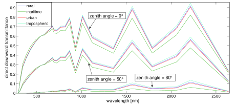
Figure 1: Direct downward transmittance (ratio between the direct downward irradiance at the Earth surface with respect to the source irradiance) vs wavelength in nm for 0^o, 50^o, 80^o source zenith angles and different aerosols conditions, in the range between 256.3 nm and 2638.5 nm. The atmosphere is in summer conditions and at midlatitudes, according to ref. [26] and the source irradiance is chosen in accordance to ref. [27]. The aerosol distributions are the rural, maritime, urban and tropospheric as described in ref. [25]. Here and in the following large scale figures the wave length resolution is kept poor in order not to compromise the readability: the code allow a much more detailed resolution than can be exploited for the region of interest (and that will be used in some smaller scale figures).

It can be observed that the best range for communications is roughly from 600 nm to almost 900 nm, but some window is present also in infrared region (as 1,564 nm or 2,214 nm).

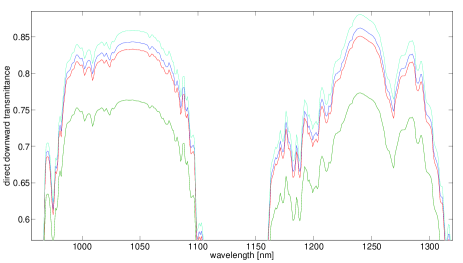
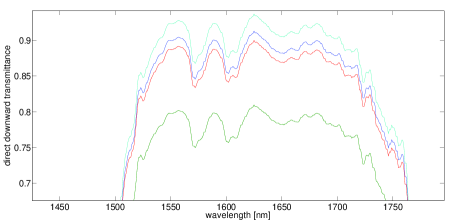
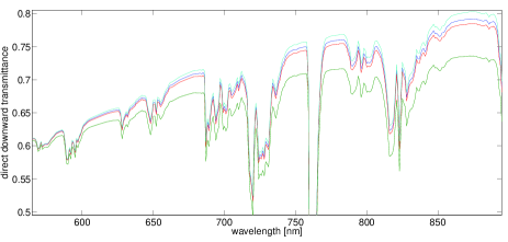
Figure 2: As in fig.1, but selecting three specific wave length windows with LOWTRAN resolution.

A detail of absorptions in some more restricted wave-length windows is shown in fig. (2), using the LOWTRAN atmospheric database. Incidentally, the use of strong resolution in wave length makes unreadable figures with a large scales and thus we only show it in lower scale figures as (2); here one can appreciate the details and clearly distinguish specific absorption lines that should be avoided for communication. On the other hand large scale figures show the rough general dependence of absorption, pointing out the regions where a more detailed analysis can be interesting.

In the range 600-900 nm, for a source zenith angle of 0^o, the fraction source light which gets across the atmosphere without any interaction with the atmosphere is, excluding some specific absorption lines (as, for instance, around 760 nm, that is due to the oxygen absorption line), about 70%.
This means that a photon has a 70% probability to get across the model of atmosphere we have built without interacting with it.
We can present, as usual, the losses in dB ($l_{dB}$), from the direct downward transmittance in percent ($T_{\%}$),

$$l_{dB}=-10\log_{10}(T_{\%})$$ (5)

Then, in the visible window from 700 nm to 900 nm, the losses due to atmospheric interaction are less than 4 dB if the source zenith angle is 0^o and less than 20 dB if the source zenith angle is 80^o, but at any rate lower than requested in [11] for establishing a secure communication. Thus, one can infer that the transmission can be carried on for almost the whole visibility range of a satellite, when the atmosphere is in the conditions we have described before.

In the following picture (3 )the losses versus the wavelength are depicted:

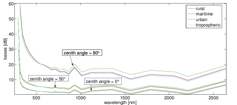
Figure 3: Losses in dB vs wavelength in nm for 0^o, 50^o, 80^o source zenith angles and different aerosols conditions, in the range between 256.3 nm and 2638.5 nm. The atmosphere is in summer conditions and at midlatitudes, according to ref. [26] and the source irradiance is chosen in accordance to ref. [27]. The aerosol distributions are the rural, maritime, urban and tropospheric as described in ref. [25]. The lowest and most constant losses are in the range from 700 nm to 900 nm

When the zenith angle is 0^o, the losses are less than 60 dB for wavelengths from 295.1 nm; when zenith angle is 50 ^o losses are around 60 dB at wavelengths equal to 295.1 nm; finally, at zenith angle equal to 80 ^o, losses are less than 60 dB only starting from 317.3 nm.

2.2 Different temperature profile

In the considered atmosphere database, the temperature decreases fairly linearly from the ground level value $T_{0}$ up to 15 km, where it assumes a given value $T_{15}$. $T_{0}$ is actually a free parameter, and we have varied its value from -10^oC up to 30^oC, with steps of 5^oC. The air density is modified according to the perfect gas law. Above 15 km, the parameters have been left unchanged, and no aerosols presence has been considered. We evaluated the Transmittance for three different source zenith angles (0^o, 50^o, 80^o). It turns out that the ground level temperature doesn’t affect the transmittance at all. Moreover, as in the previous case, the behavior of the transmittances for different level ground temperatures are largely independent of the source zenith angle. This atmosphere and the following ones are aerosol-free
So, we depict in figure (4) the results of the simulations for the source zenith angle equal to 0^o.

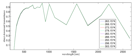
Figure 4: Direct downward transmittance (ratio between the direct downward irradiance at the Earth surface with respect to the source irradiance) vs wavelength in nm for 0^o source zenith angle, in the range between 256.3 nm and 2638.5 nm. The atmosphere is in summer conditions and at midlatitudes, according to ref. [26], but with a further modification: the surface temperature has been made vary from -10^oC up to 30^oC, with steps of 5^oC and the temperature has been decreased linearly with the altitude (for the first fifteen kilometers), up to the value it assumed in the unmodified atmosphere [26]. The source irradiance is chosen in accordance to ref. [27]. This atmosphere is considered aerosol-free

Once again, it is possible to observe that the best range for the communications is roughly from 700 nm to 900 nm as well. In fact, in this case where no aerosol was included, at a solar zenith angle of 80^o the losses are less than 14 dB. The detailed dependence, according to the LOWTRAN atmospheric database, can be observed in picture (5).

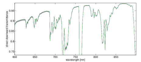
Figure 5: Detail of the figure 4, from 600 nm to 900 nm

As for the previous analysis, when the zenith angle is 0^o, the losses are less than 60 dB for wavelengths from 295.1 nm; when zenith angle is 50^o, losses are around 60 dB at wavelengths equal to 295.1 nm and then decrease as wavelengths increase; finally, at zenith angle equal to 80^o, losses are less than 60 dB only starting from 317.3 nm.
In this case, the range from 700 nm to 900 nm is the actual minimum absorbtion range in the visible wavelengths and in the picture (6), it is seen in detail (hereafter, all the detailed figures are imlied to be evaluated with the LOWTRAN database).

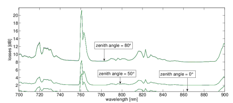
Figure 6: losses in dB vs wavelength in nm for 0^o, 50^o and 80^o source zenith angle, in the range between 700 nm and 900 nm. The atmosphere is in summer conditions and at midlatitudes, according to ref. [26], but with a further modification: the surface temperature has been made vary from -10^oC up to 30^oC, with steps of 5^oC and the temperature has been decreased linearly with the altitude (for the first fifteen kilometers), up to the value it assumed in the unmodified atmosphere [26]. The source irradiance is chosen in accordance to ref. [27]. This atmosphere is considered aerosol-free.

2.3 Different humidity profiles

In order to observe the effect of humidity, a further modification has been added to the atmospheric conditions of ref. [26]. This time, the relative humidity has been set in different times as a constant value along the first 15 km of the atmosphere. The values are 5% and from 10% to 100% with steps of 10%. No aerosols have been considered in this configuration. In figure (7), the evaluated direct downward transmittance can be observed for source zenith angles of 0^o, 50^o and 80^o.

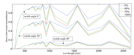
Figure 7: Direct downward transmittance (ratio between the direct downward irradiance at the Earth surface with respect to the source irradiance) vs wavelength in nm for 0^o, 50^o, 80^o source zenith angles, in the range between 256.3 nm and 2638.5 nm. The atmosphere is in summer conditions and at midlatitudes, according to ref. [26], but with a further modification: the relative humidity has been set constant along the first 15 kilometers of the atmosphere, with values of 5%, 40%, 70% and 100% values. The source irradiance is chosen in accordance to ref. [27]. This atmosphere is considered aerosol-free

Also in this scenario, the most advantageous range for communication is from 700 nm to 900 nm, where losses are less than 10 dB, but in this case we can observe some differences among different humidity conditions. As it can be observed from figure (7) and, in more details, in figure (8), the absorption in the range between 800 nm and 1000 nm is water vapor dependent and is strongly affected by its presence.

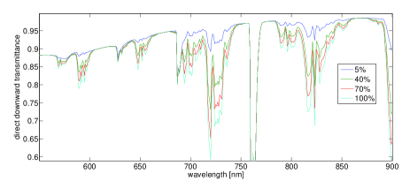
Figure 8: Detail of the figure 7, from 550 nm to 900 nm and a 0^o zenith angle

The losses in dB are depicted in figure (9),

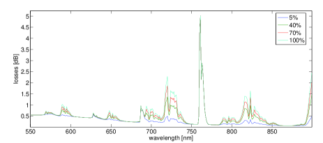
Figure 9: Losses in dB vs wavelength in nm for 0^o source zenith angle, in the range between 550 nm and 900 nm. The atmosphere is in summer conditions and at midlatitudes, according to ref. [26], but with a further modification: the relative humidity has been set constant along the first 15 kilometers of the atmosphere, with values of 5%, 40%, 70% and 100% values. The source irradiance is chosen in accordance to ref. [27]. This atmosphere is considered aerosol-free

When the zenith angle is 0^o, the losses are less than 60 dB for wavelengths from 295.1 nm; when zenith angle is 50 ^o losses are around 60 dB at wavelengths equal to 295.1 nm; finally, at zenith angle equal to 80 ^o, losses are less than 60 dB only starting from 317.3 nm.
There are minima outside the range from 700 nm to 900 nm but the former is the most stable.

2.4 Presence of clouds

In order to study the possibility of establish a quantum communication channel, the presence of clouds has to be considered as well. In order to do this, we have added clouds to the atmosphere [26] without aerosols. We set at an altitude of 10 km, a 1 km deep layer of clouds, whose liquid water content is $0.06gm^{-3}$ and the effective droplet radius is $50\mu m$. This configuration matches a cirrus and the estimation of direct downward transmittance is depicted in the figure (10).

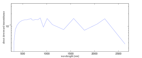
Figure 10: Direct downward transmittance (ratio between the direct downward irradiance at the Earth surface with respect to the source irradiance) vs wavelength in nm for 0^o source zenith angle, in the range between 256.3 nm and 2638.59 nm. The atmosphere is in summer conditions and at midlatitudes, according to ref. [26]. A cirrus cloud at an altitude of 10 km has been added; it is 1 km deep, with a liquid water content of $0.06gm^{-3}$ and an effective droplet radius of $50\mu m$ The source irradiance is chosen in accordance to ref. [27]. This atmosphere is considered aerosol-free

Liquid water content and effective droplet radius are translated into optical properties in [29]. As it can be seen in the figure (11), the presence of this kind of cloud doesn’t disable the communication. For 0^o and 50^o zenith angles, the losses are smaller than 60 dB starting from the 295.1 nm wavelength, nevertheless they remain always around 15-20dB. At the zenith angle of 80^o, losses are dramatically close to 60 dB. Thus, these results suggest that even the presence of thin clouds as cirri makes the transmission substantially delicate. On the other hand the presence of any other kind of clouds with a higher water content (stratus $L=0.28gm^{-3}$, cumulus $L=0.26gm^{-3}$, cumulonimbus $L=1gm^{-3}$, stratocumulus $L=0.44gm^{-3}$, …) makes the communication impossible. This information together with a description of passages of different clouds within different perturbations and statistical data on average meteorological evolution in a year for a given station allows an estimate of the available time for transmission from a specific place.

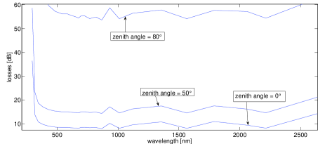
Figure 11: Losses in dB vs wavelength in nm for 0^o, 50^o and 80^o source zenith angles, in the range between 256.3 nm and 2638.5 nm. The atmosphere is in summer conditions and at midlatitudes, according to ref. [26]. A cirrus cloud at an altitude of 10 km has been added; it is 1 km deep, with a liquid water content of $0.06gm^{-3}$ and an effective droplet radius of $50\mu m$ The source irradiance is chosen in accordance to ref. [27]. This atmosphere is considered aerosol-free

The program allows a similar analysis for fog with different degrees of optical depth as well.

2.5 Comparison between two extremely different conditions

Then we want to get an idea of how is transmissivity for two extremely different conditions. On one side there is a city environment with relevant aerosols concentrations and 90% relative humidity, on the other side a dry desert without aerosols. The results for these two cases are depicted in figure (12) for source zenith angle of 0^o, 50^o and 80^o.

Figure 12: Direct downward transmittance (ratio between the direct downward irradiance at the Earth surface with respect to the source irradiance) vs wavelength in nm for 0^o, 50^o and 80^o source zenith angles, in the range between 256.3 nm and 2638.5 nm. The atmosphere is in summer conditions and at midlatitudes, according to ref. [26]. The source irradiance is chosen in accordance to ref. [27]. In the first case, there is a urban aerosol environment and a 90% relative humidity and on the other side, there is a dry desert without aerosols

As we could expect, a dry desert is a much better environment for quantum communication than a humid city. The losses in the desert are always at least 3 dB smaller than in the city
Anyway, either a dry desert and a city are secure environment for quantum communications. For 0^o and 50^o zenith angles, starting with wavelength equal to 295.1 nm, losses are lower than 60 dB, for 80^o the first secure wavelength is 317.3 nm.
We want to point out once more that the losses calculated so far, are only expect from the atmosphere. The security limit of 60 dB is a total loss limit, including, for instance, quantum efficiency of detectors, optical losses in the devices,…
For all the cases under consideration, the best range for telecommunications is from 700 nm to 900 nm.

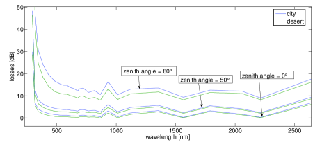
Figure 13: Losses in dB vs wavelength in nm for 0^o, 50^o and 80^o source zenith angles, in the range between 256.3 nm and 2638.5 nm. The atmosphere is in summer conditions and at midlatitudes, according to ref. [26]. The source irradiance is chosen in accordance to ref. [27]. In the first case, there is a urban aerosol environment and a 90% relative humidity and on the other side, there is a dry desert without aerosols

2.6 Quantum Entanglement over the Danube

Finally we would like to consider the realistic situation of some experiment.

As a first example, we consider a quantum entanglement distribution experiment [30] performed over the Danube in Vienna, for a distance of 600m. The information we can infer from the paper some of the meteorological conditions of when such experiment was realized, e.g. the temperature was around 0^oC and wind had strength up to 50 km/h. The bottom (at the Danube level) of the atmosphere is in summer conditions and at midlatitudes, according to ref. [26]. Urban aerosols are used. The source irradiance is chosen in accordance to ref. [27].

As an application of our program to a realistic situation, here we report the atmospheric effects for this experiment as deduced from our analysis. Although the receivers were located at a distance of either 150 m and 500 m from the source of entangled photon, we discuss the atmospheric effects over 600 m, the distance between the two receivers. The direct downward transmittance is shown in figure (14).

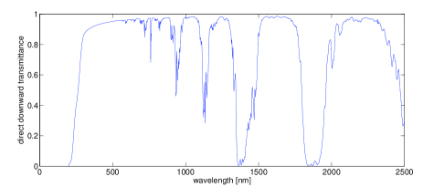
Figure 14: Direct downward transmittance (ratio between the direct downward irradiance at the Earth surface with respect to the source irradiance) vs wavelength in nm, in the range between 256.3 nm and 2638.5 nm. The bottom (at the Danube level) of the atmosphere is in summer conditions and at midlatitudes, according to ref. [26]. Urban aerosols are used. The source irradiance is chosen in accordance to ref. [27]. The path the light has to cross is 600 m long, the wind blows at 50 km/h and the surface temperature is 0^oC

For 810 nm (the wavelength in the experiment), the direct downward transmittance percentage is about 94%. In [30] it is reported that ”The attenuation in each of the links was about 12dB”, but no more indications are given about the sources of attenuation. According to our simulation, the atmospheric losses at that wavelength are less than 0.3 dB (see fig.15). We can thus suppose that the main attenuation factors were the optical

losses and finite quantum efficiency of detectors.

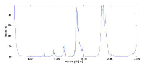
Figure 15: Losses in dB vs wavelength in nm, in the range between 256 nm and 2638 nm. The bottom (at the Danube level) of the atmosphere is in summer conditions and at midlatitudes, according to ref. [26]. Urban aerosols are used. The source irradiance is chosen in accordance to ref. [27]. The path the light has to cross is 600 m long, the wind blows at 50 km/h and the surface temperature is 0^oC. The best range is, as usual so far, from 700 nm to 900 nm

2.7 144 km transmission

As hinted in the Introduction, an ongoing experiment at Canary Islands is devoted to establish a 140 km quantum-link. Here we discuss photon transmission for a reasonable range of atmospheric conditions in a foreseen Canary Island scenario.

Generic environmental conditions are taken into considerations: the atmosphere is in summer conditions and at midlatitudes, according to ref. [26]. Maritime aerosols are used. The source irradiance is chosen in accordance to ref. [27], a 2mm monthly averaged water precipitation (value that will scale the water vapor profile accordingly).

The results of a transmission on a 144 km distance in this scenario are reported in figure (16).

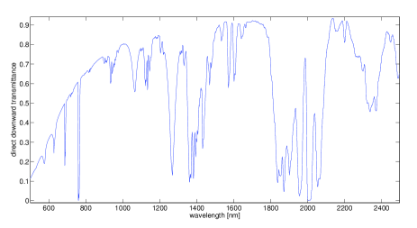
Figure 16: Direct downward transmittance (ratio between the direct downward irradiance at the Earth surface with respect to the source irradiance) vs wavelength in nm, in the range between 256.3 nm and 2638.5 nm. The scenario is at the Canary islands. The atmosphere is in summer conditions and at midlatitudes, according to ref. [26]. Maritime aerosols are used. The source irradiance is chosen in accordance to ref. [27]. The path the light has to cross is 144 km long, the average monthly precipitation is 2 mm

Results show that higher transmission percentages can be obtained for high wavelengths. Anyway, the losses are always less than 20 dB in the range from 700 nm to 900 nm.
The secure communication (losses lower than 60 dB) starts from the wavelength equal to 345.1 nm (see figure (17)).

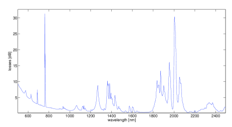
Figure 17: Losses in dB vs wavelength in nm, in the range between 256.3 nm and 2638.5 nm. The scenario is at the Canary islands. The atmosphere is in summer conditions and at midlatitudes, according to ref. [26]. Maritime aerosols are used. The source irradiance is chosen in accordance to ref. [27]. The path the light has to cross is 120 km long, the average monthly precipitation is 2 mm

From a comparison of figures 17 and 15 one can also appreciate as different atmospheric conditions (aerosols, humidity, etc.) affect specific absorption regions.

3 Conclusions

In this paper we have presented some preliminary results on atmospheric interaction with photons, obtained by using the free source library libRadtran.
Our results show that a secure communication can be established under many realistic meteorological conditions even up to only $10^{o}$ from horizon. Thus, a Earth-satellite quantum channel can be realized for a large fraction of visibility each orbit.

Furthermore, our results can be used for a first estimate of the fraction of time per year when a secure communication quantum channel with a certain satellite can be achieved.

A further deeper analysis of atmospheric effects based on this approach could effectively be a useful tool for predicting precisely the performances of a quantum communication channel in various realistic operative meteorological situations.

4 Acknowledgements

This work has been supported by Regione Piemonte (E14), by MIUR FIRB RBAU01L5AZ-002 and by ”San Paolo foundation”.

References

- [1] N. Gisin, Rev. Mod. Phys. 74 (02) 145.
- [2] S. Wiesner, Sigact News 15 (1983) 78.
- [3] C. H. Bennett, F. Bessette, G. Brassard, L. Salvail, J. Smolin, J. Cryptology 5, 3 (1992).
- [4] C. H. Bennett and G. Brassard, Int. Conf. Computers, Systems and Signal processing, Bangalore, India, p. 175 (1984).
- [5] A. K. Ekert, Phys. Rev. Lett. 67, 661 (1991).
- [6] E. Diamanti et al., quant-ph 0608110; C. Peng et al., quant-ph 0607129; I. Marcikic et al., quant-ph 0606072; C. Kurtsiefer et al., Nature 419 (02) 450; I. Marcikic et al., quant-ph 0404124.
- [7] F. Grosshans et al., Nature 421 (03) 238; D. Stucki et al., Appl. Phys. Lett. 87 (05) 194108.
- [8] C. Kim et al., quant-ph 0603013; Q. Kai, Phys. Lett. A 351 (06) 23; F.A. Bovino et al., quant-ph 0308030; M. Genovese, Phys. Rev. A 63 (01) 044303.
- [9] H. Bechmann-Pasquinucci and W. Tittel, Phys. Rev. A 61 (2000) 062308. H. Bechmann-Pasquinucci and A. Peres, Phys. Rev. Lett. 85 (2000) 3313. M.Bourennane et al., Phys. Rev. A 63 (2001) 062303.N.J. Cerf et al., Phys. Rev. Lett. 88 (2002) 127902. D. Bruss and C. Macchiavello, Phys. Rev. Lett. 88 (2002) 127901. M. Genovese and C. Novero, Eur. Journ. of Phys. D. 21 (2002) 109. A.V. Burlakov et al., Phys. Rev. A 60 (1999) R4209-R4212. M.V. Chekhova et al., Phys. Rev. A 70 (2004) 053801. J.C. Howell, A. Lamas-Linares, and D. Bouwmeester, Phys. Rev. Lett. 88 (02) 030401. A. Vaziri et al., Phys. Rev. Lett. 89 (2002) 240401. R.T.Thew et al., Phys. Rev. Lett.93 (2004) 010503.
- [10] V. N. Gorbachev, A. I. Trubilko, Laser Physics Letters Volume 3, Issue 2, Date: February 2006, Pages: 59-70.
- [11] R. Kaltenbaeck et al., ”Quantum Comm. and Quantum Imag.”, ed R. Meyers and Y. Shih, Proc. of SPIE 5161, pag. 252. P. Villoresi et al., quant-ph 0408067. M. Aspelmeyer et al., IEEE Sel. Top. Quant. El. 9 (03) 1541.
- [12] J.. Rarity et al., ”Quantum Comm. and Quantum Imag.”, ed R. Meyers and Y. Shih, Proc. of SPIE 5161, pag. 240.
- [13] P.J. Edwards et al., ”Quantum Comm. and Quantum Imag.”, ed R. Meyers and Y. Shih, Proc. of SPIE 5161, pag. 152.
- [14] G. Catastini, M. Rasetti, R. Ionicioiu, G. Brida, M. Genovese, Communication presented at ONERA workshop, Paris, April 2005.
- [15] M. Genovese, Physics Reports 413/6 (2005) 319.
- [16] G. Brida, M. Genovese, M. Gramegna, Laser Physics Letters Volume 3, Issue 3, Date: March 2006, Pages: 115-123.
- [17] C. Peng et al., Phys. Rev. Lett.94 (05) 150501; R.J. Hughes et al., La-UR-02-449; R. Alleaume et al., quant-ph 0402110.
- [18] C. Kurtsiefer et al., Nature 419 (02) 450.
- [19] T. Occhipinti, personal communication. R. Ursin et al., quant-ph 0607182.
- [20] G. Gilbert and M. Hamrick, quant-ph 0009027.
- [21] http://www.libradtran.org/
- [22] http://cfa-www.harvard.edu/hitran/.
- [23] S. Chandrasekhar, Radiative transfer (Dover, New York, 1960)
- [24] Stamnes, K., S.-C. Tsay, W. Wiscombe and K. Jayaweera, 1988, Numerically stable algorithm for discrete-ordinate-method radiative transfer in multiple scattering and emitting layered media , Applied Optics, 27, 2502.
- [25] E. P. Shettle, Models of aerosols, clouds and precipitation for atmospheric propagation studies, ”Atmospheric propagation in the UV, visible, ir and mm-region and related system aspects”, vol. 454, (1989)
- [26] G. P. Anderson, S. A. Clough,F. X. Kneizys, J. H. Chetwynd and E. P. Shettle, AFDL atmospheric constituent profiles, ”AFGL Tech. Rep., AFGL-TR-86-0110”, Air Force Geophysical Laboratories (1986).
- [27] S. Kato and T. P. Ackerman and J. H. Mather and E. E. Clothiaux, The k-distribution method and correlated-k approximation for a shortwave radiative transfer model, ”J. Quant. Spectrosc. Radiat. Transfer”, vol. 62 pp. 109-121, (1999).
- [28] P. Ricchiazzi and S. Yang and C. Gautier and D. Sowle, SBDART: A research and teaching software tool for plane-parallel radiative transfer in the Earth s atmosphere, ”Bull. Am. Met. Soc.”, vol. 79, pp. 2101-2114, (1998).
- [29] Y.X. Hu and K. Stamnes, An accurate parameterization of the radiative properties of water clouds suitable for use in climate models, ”J. Climate”, vol. 6 pp. 728-742, (1993).
- [30] Aspelmeyer A. et al., Long-Distance Free-Space Distribution of Quantum Entanglement, Science, vol. 301, no. 5633, (2003)