Direct evidence of overdamped Peierls-coupled modes
in TTF-CA temperature-induced phase transition

Abstract

In this paper we elucidate the optical response resulting from the interplay of charge distribution (ionicity) and Peierls instability (dimerization) in the neutral-ionic, ferroelectric phase transition of tetrathiafulvalene-chloranil (TTF-CA), a mixed-stack quasi-one-dimensional charge-transfer crystal. We present far-infrared reflectivity measurements down to $5$ cm^-1 as a function of temperature above the phase transition (300 – 82 K). The coupling between electrons and lattice phonons in the pre-transitional regime is analyzed on the basis of phonon eigenvectors and polarizability calculations of the one-dimensional Peierls-Hubbard model. We find a multi-phonon Peierls coupling, but on approaching the transition the spectral weight and the coupling shift progressively towards the phonons at lower frequencies, resulting in a soft-mode behavior only for the lowest frequency phonon near the transition temperature. Moreover, in the proximity of the phase transition, the lowest-frequency phonon becomes overdamped, due to anharmonicity induced by its coupling to electrons. The implications of these findings for the neutral-ionic transition mechanism is shortly discussed.

I Introduction

In a formulation similar to a student’s exercise, more than fifty year ago Rudolf Peierls pointed out that one-dimensional (1D) metals are intrinsically unstable with respect to lattice distortions opening a gap at the Fermi energy.peierls It did not take long to realize that the quasi-1D electronic structure of organic charge-transfer (CT) conductors offers an almost ideal model for the Peierls mechanism. Extensive investigations in the 1970s revealed that the Peierls instability may occur also in 1D Mott insulators, due to coupling of the lattice to spin (spin-Peierls),mcconnell or to both electronic and spin degrees of freedom (“generalized” Peierls instability).bray At the time, the attention was almost exclusively devoted to segregated-stack CT crystals, where identical electron-donor (D) or acceptor (A) $\pi$-molecules are arranged face-to-face along one direction. Mixed stacking (…DADA…) received far less attention, at least until a new kind of phase transition was discovered in these systems: the so-called neutral-ionic phase transition (NIT).nitP ; nitT It is characterized by a change in the ionicity $\varrho$, i.e. the charge transfer from D to A in the ground state. Temperature $T$ or pressure $p$ may induce a change from a quasi-neutral N, $\varrho\lesssim$ 0.5) to a quasi-ionic (I, $\varrho\gtrsim$ 0.5) ground state. It was early recognized that the ionic state is subject to the Peierls instability, yielding a stack dimerization (..DA DA DA..).GP86 ; nagaosa86

NIT are complex phenomena, resulting from the interplay between two order parameters, the ionicity $\varrho$ and the dimerization $\delta$, and present a rich and intriguing phenomenology.ricemem ; tokurareview Some of the phenomena occurring on approaching the phase transition, like the dramatic increase of the dielectric constant or the observation of diffuse scattering signals in x-ray diffraction,TTFCAdiel ; buron06 have been recently ascribed to charge oscillations associated with the soft mode that yields the stack dimerization, namely, the Peierls mode.freo02 ; soos04 ; davino07 It is then of fundamental importance to identify the Peierls mode in order to confirm the above suggestion and to shed light on the NIT mechanism. At variance with segregated stack crystals, the Peierls mode is optically active in mixed stack structures,GP86 which offers a rather unique possibility for its optical detection and characterization. Finally, since the dimerized ionic stack is potentially ferroelectric,tokura89 the Peierls mode is the counterpart of the so-called ferroelectric mode of perovskite-type crystals.nakamura66

Direct and clear experimental identification and characterization of the Peierls mode and of its role in the NIT has proved to be more difficult than expected.moreac96 ; okimoto01 One of the reasons is that the phonon structure of molecular crystals is very complex, and several modes are likely coupled to CT electrons. Therefore the analysis of the spectra requires a detailed and reliable understanding of the lattice-phonon dynamics. We have recently undertaken such analysis for tetrathiafulvalene-chloranil (TTF-CA), which undergoes a first-order temperature induced NIT at 81 K.ricemem In a first paper (hereafter Paper I)paperI we presented a quasi harmonic lattice dynamics (QHLD) calculations of TTF-CA lattice phonons above and below the transition temperature, and gave a first partial interpretation of the infrared (IR) and Raman spectra.

The specific goal and achievement of the present paper is the identification of the Peierls (soft) modes in TTF-CA neutral phase. We present detailed and improved data for single crystals of TTF-CA in the spectral region $5-200$ cm^-1 collected in the temperature range down to 82 K. Particular attention is devoted to the submillimeter spectral range, below 30 cm^-1. The experimental data are analyzed in terms of a multi-mode Peierls model, that combines the information on lattice phonon dynamics reported in Paper I,paperI with that on the electronic structure as obtained from the exact diagonalization of the 1D Peierls-Hubbard Hamiltonian in Ref. soos04, . The model fully accounts for the experimental data and allows us to demonstrate that mode mixing and overdamping are the key to explain the changes of the far-IR spectra on approaching the transition. The effective Peierls mode detected by an analysis of the combination modes in the mid-IR regionsidebands is also accounted for. In addition, the dielectric constant anomaly at the transitionTTFCAdiel is quantitatively reproduced.

II Experimental methods

TTF-CA single crystals were grown by sublimation. Crystals as large as $4~{}{\rm mm}\times 4~{}{\rm mm}$ allowed for measurement down to 5 cm^-1. The reflectivity was probed on well-developed naturally grown $ab$ crystal faces along the optical axes. The crystals were oriented at room temperature according to the known spectra in mid-IR region, using a Hyperion IR microscope attached to Bruker IFS66v Fourier-transform spectrometer. In this paper we present the spectra polarized parallel to the $a$ stack axis; only these spectra are relevant to the analysis of Peierls coupling in the neutral phase.paperI

The reflectivity spectra were collected by three different setups and techniques, depending on the spectral region of interest: (i) In the $5-30$ cm^-1 region, we employed a quasi-optical submillimeter spectrometer, equipped with backward wave oscillator as coherent and tunable source; a Golay-cell served as a detector. Temperature dependent measurements were conducted in an exchange-gas helium cryostat. The absolute reflectivity was obtained by comparing sample reflectance to reflectance of an aluminum mirror fixed on the same aperture. The spectral resolution in this range is better than 0.01 cm^-1. (ii) In the $20-150$ cm^-1 range the reflectivity was measured by a Bruker IFS66v with a spectral resolution of 0.5 cm^-1. The spectrometer was equipped with 1.4 K Si bolometer and a CryoVac cold-finger cryostat. The sample was fixed on the cold finger by carbon paste; a good temperature contact was ensured by Apiezon paste. To get absolute values of reflectivity, the in-situ gold-evaporation technique was adopted:homes93 after measuring the temperature dependence of the sample reflectivity, gold is evaporated onto the sample surface, and used as reference. (iii) Reflectance measurements in the $100-6000$ cm^-1 range were done in a Bruker IFS 113v FTIR spectrometer equipped with a 4.2 K Si bolometer, an MCT detector, and an exchange-gas helium cryostat. The absolute reflectivity values of the sample have been obtained by a comparison to a Au mirror of the same size. In this spectral range a resolution of 2 cm^-1 was chosen. The reflectivity values agree well with available literature data,jacobsen83 which extend from 3000 to 14 000 cm^-1 and thus cover the charge transfer transition. The extension to high wavenumbers is needed to obtain reliable Kramers-Kronig transformation (KKT) of the data.

We ensured that good overlap exists between the data measured in the three spectral regions. In order to match the absolute values, the submillimeter data were rescaled to those obtained by the Bruker IFS66v FTIR because the in-situ gold-evaporation technique ensures the most precise measurements of the absolute reflectivity and does not depend on the quality of the sample surface.

In the KKT analysis the data were extrapolated below 5 cm^-1 to fit the known values of the static dielectric constant $\epsilon_{1}$.TTFCAdiel We also verified that an extrapolation to a constant value does not significantly affect the portion of the spectra for which experimental data exist. At frequencies above 14 000 cm^-1 an extrapolation $R(\omega)\propto\omega^{-2}$ has been used.

III Reflectivity spectra

III.1 Spectral data

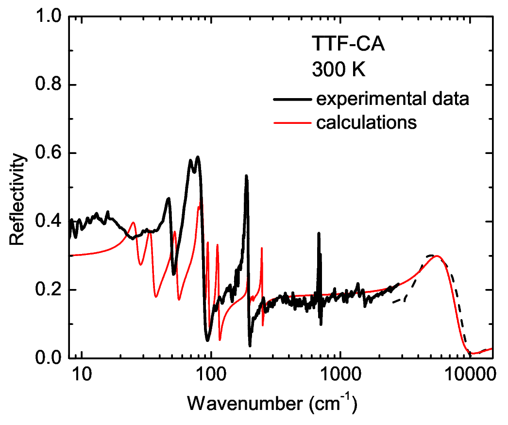
Figure 1: (color online) Experimental and calculated (Section V) reflectivity spectra of TTF-CA at $T=300$ K, with the polarization $E\parallel a$. The spectral region above 3000 cm^-1 (dashed curve) is taken from Ref. jacobsen83, . Notice the logarithmic frequency scale.

Fig. 1 shows the room temperature TTF-CA reflectivity along the stack axis for the whole measured spectral range, with extension to 14 000 cm^-1 taken from Ref. jacobsen83, . The reflectivity is rather low, as expected for a non-metallic compound. The charge transfer electronic transition occurs around 5000 cm^-1  and at lower frequencies reflectivity gets down to about 0.2, with no relevant feature observed until we encounter the highest frequency out-of-plane intramolecular modes, at 701 and 682 cm^-1, corresponding to CA and TTF, respectively.girlando83 Below 250 cm^-1 we find a couple of other modes of prevailing out-of-plane, intramolecular character, and finally the intermolecular modes we want to discuss in detail in the present paper.

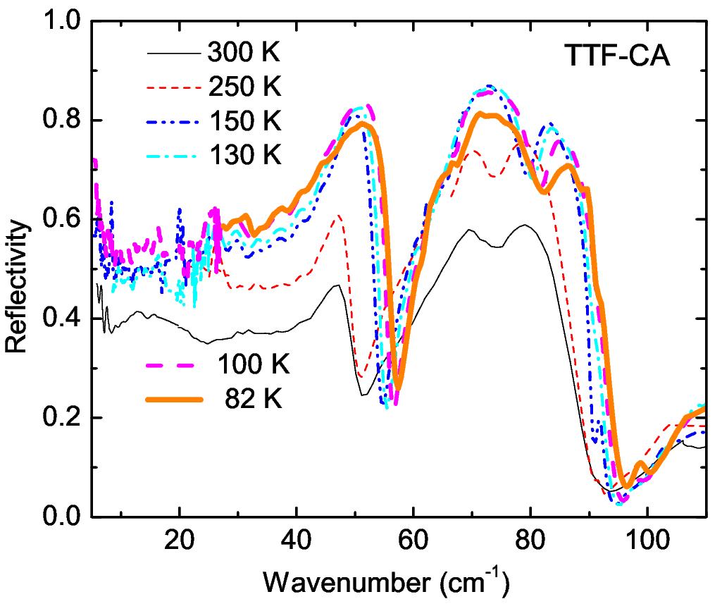
Figure 2: (color online) Reflectivity spectra of TTF-CA single crystal along the $a$ axis taken at different temperatures $T>T_{c}$ above the N – I transition.

The temperature dependence of the low-frequency ($5-120$ cm^-1) reflectivity spectra is presented in Fig. 2. At room temperature a group of strong phonon bands is observed just below 100 cm^-1. At lower frequencies the reflectivity remains approximately at the level of 0.4 down to the lowest measured data (5 cm^-1 ). On cooling the sample from 300 to 82 K, the reflectivity above 120 cm^-1 reveals only unimportant changes, and is therefore not reported. Instead Fig. 2 shows that dramatic changes occur below 100 cm^-1, where reflectivity rises by 1.5 times on lowering temperature to 82 K, just before the NIT. As demonstrated in Paper I,paperI below the transition temperature ($T_{c}$ = 81 K) the reflectivity drops down to values below those at $T=300$ K, and does not change considerably on further cooling to 10 K.

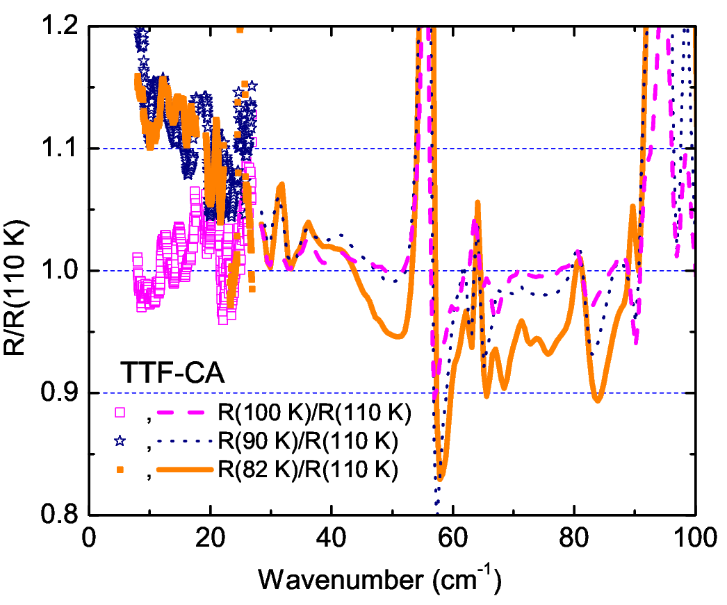
Figure 3: (color online) Ratio of the of the reflectivity spectra at 82, 90, and 100 K to the reflectivity at 110 K. Measurements in the range below 25 cm^-1 performed by using the submillimeter spectrometer (points), data above 25 cm^-1 collected by using Bruker 66v spectrometer (lines). Note the increase of reflectance below 25 cm^-1 at temperatures close to the N – I transition temperature.

A more detailed inspection of Fig. 2 provides evidence that the strongest increase of reflectivity, from about 0.4 to 0.6, occurs on cooling between 300 and 150 K. Some increase of reflectivity below approximately 40 cm^-1 occurs on further cooling, indicating a shift of spectral weight to lower frequencies. The quality of the data in the low-frequency region, essential to appreciate the shift of spectral weight, is illustrated in Fig. 3, where the reflectivity at $T$ = 82, 90 and 100 K is normalized to the reflectivity at 110 K. This figure illustrate the good overlap between submillimeter and FIR data, collected with two different instrumentations (see Section II). The reflectivity ratio $R(T)/R(110~{}{\rm K})$ for these two spectral regions have indeed differences smaller than the noise of the measurements. Thus we safely confirm that by lowering $T$ below 100 K the reflectivity drops in the range 30-100 cm^-1 range and increases below, with a redistribution of the overall spectral weight.

III.2 Optical conductivity

Frequency dependent conductivity spectra, obtained by the KKT of the reflectivity, are presented in Fig. 4. In order to better understand the temperature evolution of the conductivity spectra, and to gain confidence in the band assignment, we have also fitted the original reflectivity data with a set of Lorentzians. The resulting conductivity practically coincides with the KKT conductivity, as exemplified for the 300 and 82 K data in the upper panel of Fig. 5. The individual Lorentzians used in the deconvolution are also shown. In the bottom panel of the Figure we report an enlarged view of the temperature evolution of the KKT conductivity vs. the multi-Lorentzian reflectance fit. The logarithmic scale for the wavenumber axis focus attention on the deconvolution of the lowest frequency phonon mode, that we shall discuss in detail below.

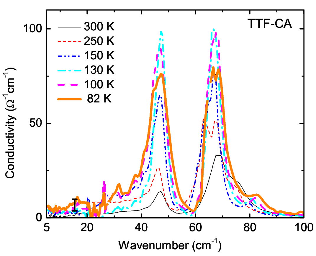
Figure 4: (color online) Conductivity spectra along the $a$ stack axis at temperatures above the N – I transition. An error bar for the absolute values of low frequency conductivity is shown.

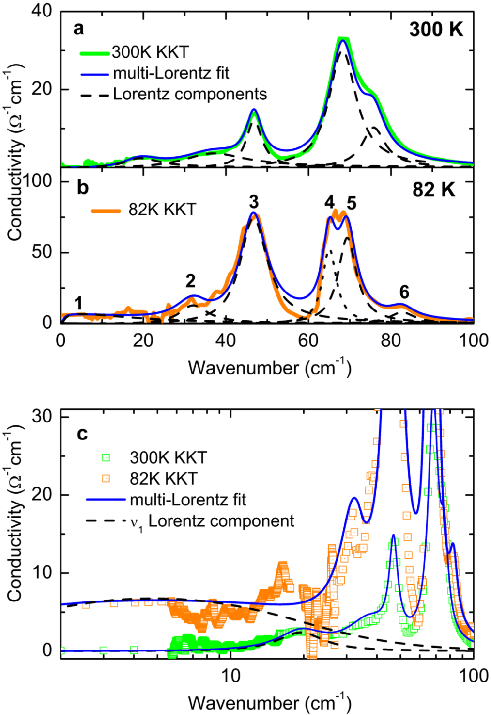
Figure 5: (color online) Upper panel: Comparison of the TTF-CA KKT conductivity at 300 K (green line) and 82 K (orange line) with the fit of reflectivity spectrum by a minimum number of harmonic oscillators. The Lorentzian bands used in the deconvolution are shown as dashed lines, and the resulting conductivity as blue lines. Bottom panel: Comparison of the KKT conductivity with the multi-Lorentzian fit at two different temperatures. The Lorentz component of the lowest frequency phonon ($\nu_{1}$) is also shown. Notice the wavenumber logarithmic scale.

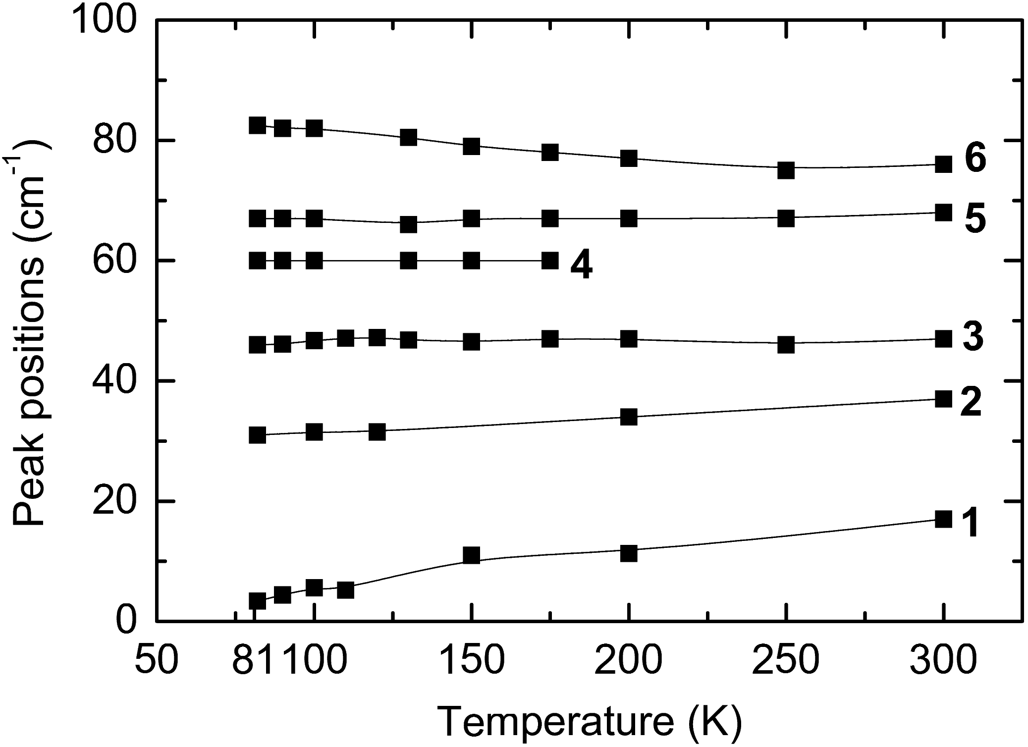
Figure 6: Temperature dependence of the frequencies of the six phonons bands observed below 100 cm^-1, labeled $\nu_{1}$ to $\nu_{6}$ going from the lowest to the highest frequency.

Six peaks are clearly identified in the spectral region below 100 cm^-1. We label them $\nu_{1}$ to $\nu_{6}$ in order of increasing frequency, as shown in the upper panel of Fig. 5. The temperature evolution of the $\nu_{1}$ to $\nu_{6}$ peak frequencies is reported in Fig. 6. In a group of bands with a broad maximum around 68 cm^-1 at $T=300$ K, we resolve three modes ($\nu_{6},\nu_{5}$ and $\nu_{4}$) at lower temperatures. While the high-frequency band shows normal hardening on lowering $T$, the $\nu_{5}$ and $\nu_{4}$ modes essentially do not change their positions. The $\nu_{3}$ band at 47 cm^-1 exhibits a very weak softening of 2 cm^-1 below $T=130$ K. The deconvolution of the low frequency region of the room temperature spectrum suggests the presence of bands around 32 and 17 cm^-1 ($\nu_{2}$ and $\nu_{1}$), “appended” to the 47 cm^-1 band. When going from ambient $T$ to 200 K, the $\nu_{1}$ band shifts below 15 cm^-1 and becomes wider. It shifts to even lower frequencies and broadens as temperature is reduced, getting down to about 5 cm^-1 for $T=90$ K (Fig. 6), assuming the shape of a broad background at temperatures just above the phase transition (Fig. 5, bottom panel).

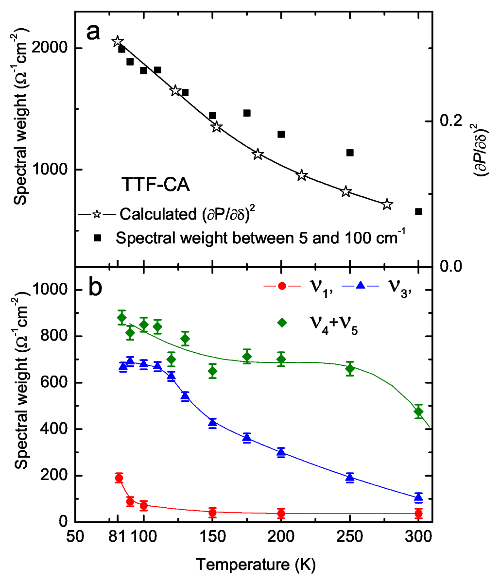
Figure 7: (color online) (a) Temperature dependence of the spectral weight of the $0-100$ cm^-1spectral region (squares), compared with the temperature dependence of $(\partial P/\partial\delta)^{2}$ (open stars) (Section V). (b) Temperature dependence of the spectral weight of the group of bands around 70 cm^-1($\nu_{4}$ and $\nu_{5}$) (rhombs), and of the $\nu_{3}$ (triangles) and $\nu_{1}$ (circles) bands. The lines are a guidance to the eye.

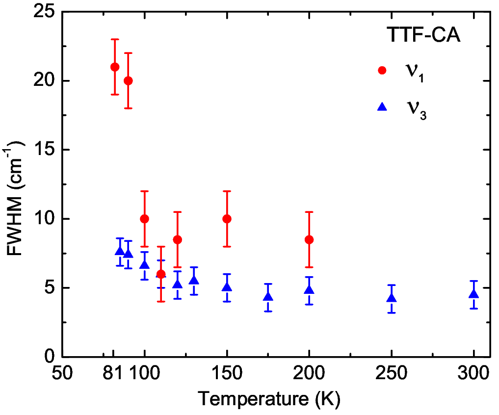
Figure 8: (color online) Temperature dependence of the full width at half maximum (FWHM) of the $\nu_{1}$ (circles) and of the $\nu_{3}$ (triangles) bands in TTF-CA.

The conductivity spectra in Fig. 4 show a huge increase of overall intensity by lowering $T$. A quantitative estimate of this growth in terms of the spectral weight between 0 and 100 cm^-1 is shown in Fig. 7a. The intensities of the individual bands, estimated by integrating in the relevant spectral region, are reported in the lower frame. Fig. 7b shows that only some bands gain intensity by lowering $T$: the $\nu_{5}$ and $\nu_{4}$ (estimated as a whole maximum around 70 cm^-1  since the bands are not well resolved), the $\nu_{3}$ band at 47 cm^-1, and the $\nu_{1}$ band. The intensity of the latter increases only below 100 K.

While the spectral weight increases on cooling, it also redistributes towards lower frequency bands. The temperature dependence of intensity around 70 cm^-1 has smaller slope below 200 K, whereas the spectral weight of $\nu_{3}$ (47 cm^-1) band saturates at temperatures below 130 K. At this temperature the intensity of the $\nu_{1}$ band starts to rise rapidly. Just above the transition, from 90 to 82 K, the $\nu_{1}$ band grows at the expenses of the $\nu_{3}$ one.

With lowering temperature the $\nu_{3}$ and $\nu_{1}$ bands show considerable anharmonicity. While at $T=300$ K the $\nu_{3}$ band (47 cm^-1) can still be fitted with a Lorentzian, it becomes wider and very asymmetric at temperatures below 250 K, as its lower frequency wing grows on cooling. The temperature dependence of the full width at half maximum (FWHM) of the $\nu_{3}$ band, directly estimated from experimental spectra (Fig. 5, bottom panel), is displayed in Fig. 8. The same plot shows also the dramatic increase of the FWHM of the lowest frequency $\nu_{1}$ band below $T$=100 K, with clear overdamping at temperatures close to the transition.

The present analysis of the spectra evidences a very specific behavior of $\nu_{5}$, $\nu_{4}$, and especially $\nu_{3}$ and $\nu_{1}$ bands as the temperature approaches the NIT. The bands clearly correspond to the most strongly coupled Peierls modes. By lowering $T$, they show a huge intensity increase, with a concomitant intensity redistribution, and important deviations from Lorentzian bandshape. Below 100 K, we also observe appreciable softening and large broadening for the lowest frequency mode. A quantitative explanation of this complex temperature behavior of the spectrum is offered by the model discussed in Section V, while in the next Section we describe the computational methods.

IV Computational methods

The separation of intramolecular vibrations from intermolecular, or lattice, phonons is a common and useful approximation in dealing with the complex phonon spectra of molecular crystals. Thus lattice phonons describe translations and rotations of the rigid molecules (rigid molecule approximation, RMA). In the framework of a Hubbard-model description of the electronic structure (see below), the electron-phonon coupling can also be separated into two contributions: The totally symmetric molecular vibrations are assumed to couple with electrons through modulation of on-site energies (electron-molecular vibrational, or Holstein, coupling). On the other hand, lattice phonons and possibly out-of-plane molecular vibrations are expected to modulate the inter-molecular CT integral (Peierls coupling).e-ph

In order to characterize the Peierls coupling in TTF-CA, we have first calculated the lattice phonon frequencies and normal coordinates at $T=300$ K (N phase) by the quasi-harmonic lattice dynamic (QHLD) method, as described in paper I.paperI The atom-atom potential adopted in QHLD accounts for van der Waals and Coulomb forces, but does not include the CT interaction. It should be noted that in the calculation we have relaxed the RMA, by actually considering all the phonons below $\sim 250$ cm^-1.

We describe the strength of Peierls coupling in terms of the linear Peierls-coupling constants:

$$g_{i}=\sqrt{\frac{\hbar}{2\omega_{i}}}\left(\frac{\partial t_{\rm DA}}{{\partial Q_{i}}}\right)_{eq}$$ (1)

where $t_{\rm DA}$ is the CT integral between adjacent DA molecules along the stack, and $Q_{i}$ is the normal coordinate for the $i$-th phonon with frequency $\omega_{i}$ and wavevector $\textbf{q}=0$. The CT integral and its variation with $Q_{i}$ has been calculated by the extended Hückel method, adopting the Wolfsberg and Helmholtz approximation.EH At the room-temperature equilibrium geometry, we find $t$ = 0.20 eV, in agreement with current estimates.soos04 The $g_{i}$ values, obtained by numerical differentiation, offer a reliable indication of the relative magnitude of the coupling constants. The Peierls coupling strength of the $i$-th phonon is given by $\varepsilon_{i}=(g_{i}^{2}/\omega_{i})$, and the total coupling strength, or lattice relaxation energy, is $\varepsilon_{\rm d}=\sum_{i}\varepsilon_{i}$.

The electronic structure of TTF-CA is described in terms of a modified Hubbard model with adiabatic coupling to molecular and lattice vibrations. Real space diagonalization of the modified Hubbard Hamiltonian relevant to stacks of up to 18 molecules with periodic boundary conditions yields reliable information on the ground state properties.soos04 The expectation value of the dipole moment operator and its derivatives are calculated by the Berry-phase approach.soos04

V Spectral modeling

As discussed in Paper I paperI and elsewhere,moreac96 ; lecointe95 in the N phase of TTF-CA the Peierls-coupled phonons transform as the $B_{u}$ species in the $C_{2h}^{5}$ crystal symmetry, and are IR active with polarization along the stack axis. We shall therefore restrict our attention to these phonons. In Table 1 we list the QHLD calculated $B_{u}$ frequencies for the equilibrium structure at 300 K,paperI and the corresponding coupling constants and coupling strength obtained as described in Section IV. The total coupling strength, or lattice relaxation energy, is $\varepsilon_{\rm d}=0.1$ eV. Phonons above 250 cm^-1 give negligible contribution to $\varepsilon_{\rm d}$. As a consequence, they are not reported in the Table nor discussed here.

Table 1: Calculated low-frequency $B_{u}$ phonons of TTF-CA in the N phase. $\omega_{i}$, $g_{i}$, and $\varepsilon_{i}$ denote the zero-order frequency, Peierls coupling constant, and coupling strength, respectively.

	mode	$\omega_{i}$ (cm-1)	$g_{i}$ (meV)	${\varepsilon}_{i}$ (meV)
$B_{u}$	$\nu_{1}$	27.6	$-5.16$	7.8
	$\nu_{2}$	38.6	$8.30$	14.4
	$\nu_{3}$	55.8	$-8.68$	10.9
	$\nu_{4}$	80.5	$-2.16$	0.5
	$\nu_{5}$	90.5	$-9.66$	8.3
	$\nu_{6}$	99.4	$-16.99$	23.4
	$\nu_{7}$	113.2	$-2.27$	0.4
	$\nu_{8}$	118.5	$-20.71$	29.2
	$\nu_{9}$	134.0	$0.08$	0.0
	$\nu_{10}$	194.3	$7.85$	2.6
	$\nu_{11}$	206.0	$-2.43$	0.2
	$\nu_{12}$	211.3	$-2.93$	0.3
	$\nu_{13}$	250.7	$-13.75$	6.1

As already mentioned in Section IV, the QHLD internuclear potential does not include the CT interaction, so that values in Table 1 are the zero-order reference frequencies in the absence of Peierls coupling. In other words, they correspond to an hypothetical state with $\varepsilon_{d}=0$ or, equivalently, to a state where the electronic excitations are moved to infinite energy.e-ph As a consequence, the frequencies of Table 1 cannot be directly compared to the experimental frequencies. In fact, phonons with high values of coupling constants are expected to be the most intense in the spectra, and to occur at frequencies lower than the zero-order ones. Therefore we can for instance anticipate that the $\nu_{6}$ and $\nu_{8}$ modes of Table 1 correspond to the group of intense bands occurring around 70 cm^-1 (Fig. 4). Incidentally, the eigenvectors of the $\nu_{6}$ phonon correspond to rigid molecular displacements along the stack, whereas the $\nu_{8}$ phonon has a more complex description, being a mixture of TTF torsional motion and molecular displacement along the stack. Modes above 200 cm^-1, on the other hand, are almost pure intramolecular modes, like for instance the $\nu_{13}$ phonon, which essentially corresponds to a TTF out-of-plane motion. Their intensity may then have a significant “intrinsic” contribution (namely, not due to Peierls coupling), that is not accounted for in the present model calculation.

Both experiment and calculations suggest that several modes are appreciably coupled to the CT integral, leading to a multi-mode Peierls coupling. The resulting problem becomes complex because the phonons are mixed through their common interaction with the CT electrons. Thus a meaningful comparison with experiment requires detailed modeling. The effect of Peierls coupling can be dealt with separately for the phonon frequencies and for their IR intensity.soos04 Accordingly, the analysis will be carried out in two steps.

Table 2: Calculated electronic response $\chi_{b}$ and squared polarizability derivative $(\partial P/\partial\delta)$ for different degree of ionicity $\varrho$. The correspondence between $\varrho$ and $T$ is derived from experiment (Ref. sidebands, ).

$\chi_{b}$ (eV-1)	$(\partial P/\partial\delta)^{2}$	$\varrho$		$T$ (K)
5.7971	0.0858	0.197		277
6.1230	0.1034	0.209		247
6.4862	0.1257	0.222		215
6.8944	0.1544	0.236		183
7.3561	0.1919	0.250		153
7.8837	0.2415	0.266		123
8.4927	0.3089	0.282		81

It has been shown that in the presence of Peierls electron-phonon interaction, the squared perturbed frequencies $\Omega_{j}^{2}$ and normal modes coordinates $\mathcal{Q}_{j}$ are obtained from the diagonalization of the following force constant matrix, written in the basis of the reference coordinates $Q_{i}$:pg88

$$F_{ij}=\omega_{i}\omega_{j}\delta_{ij}-\sqrt{\omega_{i}\omega_{j}}~{}g_{i}g_{j}~{}\chi_{b}.$$ (2)

In this equation, $\omega_{i}$ and $g_{i}$ are the reference frequencies and coupling constants of Table 1, and $\chi_{b}$ is the electronic response to phonon perturbation. The $\chi_{b}$ values needed to apply Eq. 2 are calculated as described in Ref. soos04, by tuning the parameters of the modified Hubbard model as to mimic the behavior of TTF-CA. Since in going from 200 to 82 K the TTF-CA ionicity $\varrho$ changes from about 0.2 to 0.3;girlando83 ; sidebands in the first column of Table 2 we list the $\chi_{b}$ values corresponding to different ionicities in this interval. By matching the calculated ionicities in the third column of the Table with the experimental ones,sidebands we can translate the $\varrho$-dependence of the calculated $\chi_{b}$ in a $T$-dependence, as reported in the fourth column of Table 2. In this way we can perform a more direct comparison with experimental data.

Fig. 9 summarizes the temperature dependence of the perturbed frequencies $\Omega_{j}$ below 100 cm^-1  calculated through Eq. (2), with the parameters listed in Tables 1 and 2. The agreement between the calculated frequencies in Fig. 9 and the experimental ones presented in Fig. 6 is very good. First of all, the number of modes below 100 cm^-1 is the same, namely six. Second, an appreciable softening is detected only for the lowest frequency mode, and in the proximity of the phase transition. The weak softening shown by some higher frequency modes in Fig. 9 is likely compensated by the usual frequency hardening by lowering $T$, a factor not included in the model.

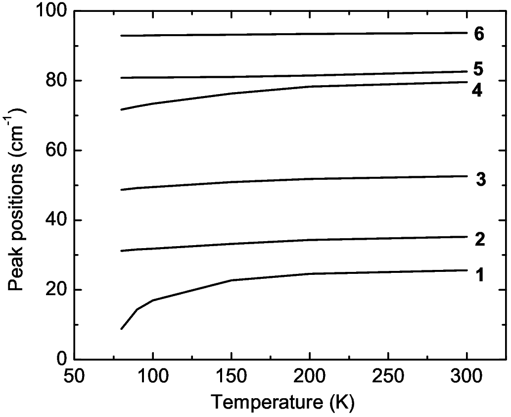
Figure 9: Temperature dependence of the Peierls-coupled modes, calculated by Eq. (2), on the basis of Table 1 and Table 2 parameters.

The calculations quite naturally explain why – although several phonons are coupled to the CT electrons – the red shift of the associated bands on getting close to the transition is so small. As mentioned above, all the phonons are coupled together through their common interaction with the electronic system. Then, when two phonon frequencies get closer due to a softening of the higher frequency phonon, there is mixing in the phonon description, and the softening is “transferred” to the lower frequency phonon. In more precise terms, with lowering temperature $\chi_{b}$ increases with $\varrho$ (Table 2), leading to an evolution of the normal modes $\mathcal{Q}_{j}$:

$$\mathcal{Q}_{j}=\sum_{i}l_{ij}Q_{i},$$ (3)

where $l_{ij}$ are the eigenvectors obtained, for each temperature, by diagonalizing the F matrix of Eq. 2. The Peierls coupling constants are accordingly modified: The coupling constants $G_{j}$ in the basis of the perturbed normal modes $\mathcal{Q}_{j}$ are linear combination of the reference coupling constants:

$$G_{j}=\sum_{i}l_{ij}g_{i}\sqrt{\frac{\omega_{i}}{\hbar}},$$ (4)

and therefore evolve with $\chi_{b}$. As a result, on approaching the phase transition the coupling strength is progressively transferred to the lower frequency modes. Only in close proximity of the transition all the coupling strength collapses to the lowest frequency phonon, yielding substantial softening of this specific mode.

We now turn our attention to the intensity of the phonon bands. For a regular stack (equispaced D and A units along the stack, like N TTF-CA) the IR intensity of the Peierls modes is largely dominated by a term accounting for the charge fluctuations induced by oscillation in the dimerization amplitude $\delta$. For a single Peierls mode with frequency $\omega_{\mathrm{P}}$ the total oscillator strength is:soos04

$$f_{\mathrm{P}}=\frac{m_{e}d^{2}\omega_{\mathrm{P}}^{2}\varepsilon_{\rm d}}{t^{2}}\left(\frac{\partial P}{\partial\delta}\right)^{2},$$ (5)

where $m_{e}$ is the electronic mass, $d$ the equilibrium distance between D and A molecules, and $P$ the electronic polarizability per site. The $(\partial P/\partial\delta)^{2}$ values calculated for parameters relevant to N TTF-CA are reported in the second column of Table 2. The temperature dependence of the $(\partial P/\partial\delta)^{2}$ terms compares well with the experimentally determined growth of the spectral weight in the range of 0-100 cm^-1 (Fig. 7).

In the multi-mode Peierls coupling case, the oscillator strength is partitioned among the coupled modes. Specifically, each normal coordinate $\mathcal{Q}_{j}$ modulates the CT integral as described by the coupling constants $G_{j}$ in Eq. (4). Using the usual chain-rule, the $\delta$-derivative of $P$ in Eq. (5) can be rewritten as a sum of $\mathcal{Q}_{j}$ derivatives. After some algebra we derive the following expression for the IR oscillator strength of each mode coupled to the electronic degrees of freedom:

$$f_{j}=\frac{m_{e}d^{2}}{t^{2}}~{}G_{j}^{2}\left(\frac{\partial P}{\partial\delta}\right)^{2}.$$ (6)

We can now use the standard expression for the frequency-dependent dielectric constant

$$\epsilon(\omega)=\epsilon_{\infty}+8.96857\cdot 10^{10}~{}\frac{N}{V}\sum_{k}\frac{f_{j}}{(\Omega_{j}^{2}-\omega^{2})-\mathrm{i}\omega\Gamma_{j}}$$ (7)

to calculate the contribution of the Peierls coupled modes to the low-frequency spectra of TTF-CA. The numerical factor in Eq. (7) refers to $N/V$ (number of molecules per unit-cell volume) expressed in Å^-3, and the frequencies $\Omega_{j}$, $\omega$, and damping $\Gamma_{j}$, in cm^-1.

The calculated reflectivity is compared to the experimental one in Fig. 1 of Section III.1. The unperturbed frequencies and coupling constants needed for the calculation are taken from Tab. 1, whereas $\Gamma_{j}$ is set equal to 4.0 cm^-1 for all the modes. The values of $\chi_{b}$ = 5.6667 eV^-1 and $(\partial P/\partial\delta)^{2}$ = 0.07922 are obtained from interpolation of the data in Tab. 2. In addition, we use $d=3.7$ Å, $N/V=4.92386\cdot 10^{3}$ Å^-3 (Ref. lecointe95, ), and $t=0.2$ eV. The CT electronic transition is added in the calculation as an extra term in Eq. (7), where $f_{\rm CT}$, $\Omega_{\rm CT}$ and $\Gamma_{\rm CT}$ are derived directly from experiment.jacobsen83 Finally, we put $\epsilon_{\infty}=2.5$ to account for the high-energy contributions.

Fig. 1 shows a very good agreement between model calculation and experiment, considering all the approximations involved in the model and in the estimate of the parameters, in particular of the $g_{i}$. The frequencies are somewhat off, but well within the usual errors of QHLD calculations ($\pm$ 10 cm^-1). The calculated oscillators strengths for the lower frequency modes are just a little below the experiment. The agreement for the oscillator strength of the phonons at higher frequencies is not expected to be exact, because these phonons have intra-molecular character and, as discussed above, may have a non-negligible “intrinsic” intensity. The simulation indicates that at room temperature the most strongly coupled modes cluster around approximately $70-80$ cm^-1.

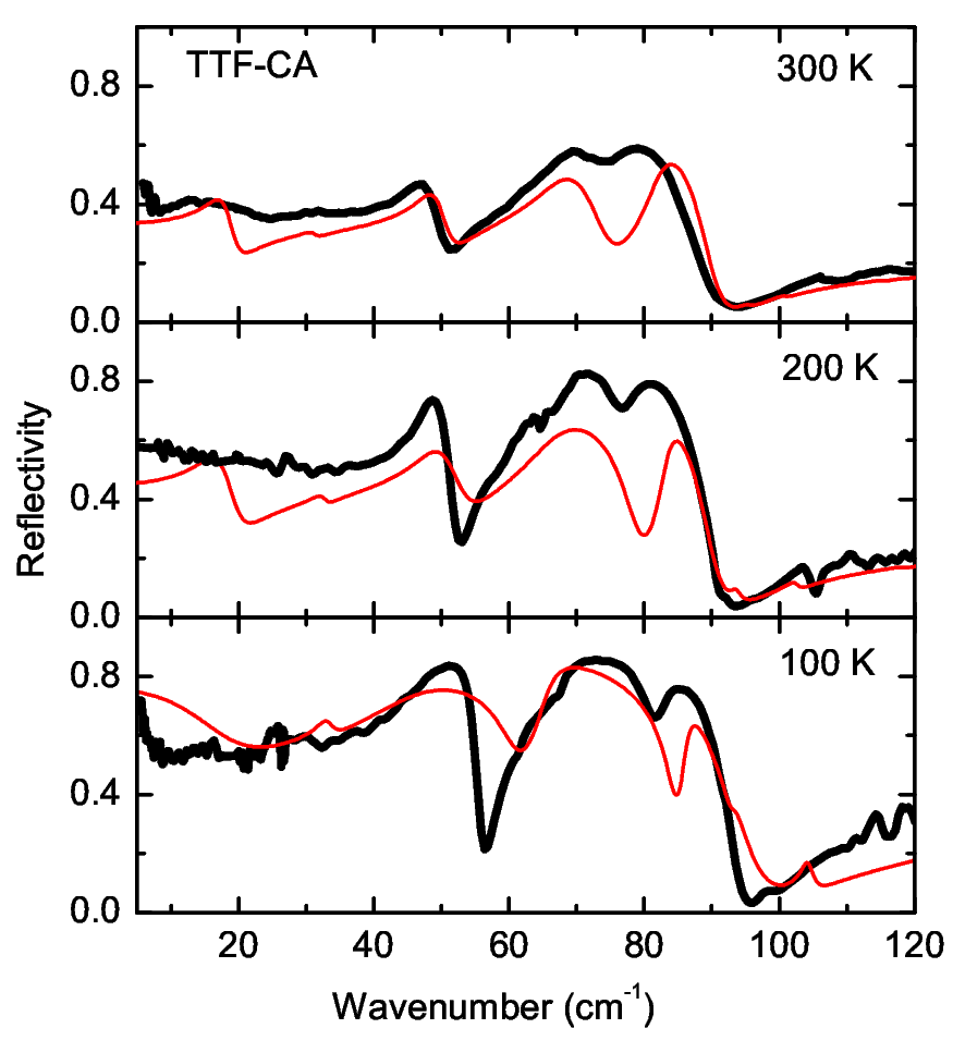
Figure 10: Experimental (thick line) and calculated (thin line) low-frequency reflectivity spectra of TTF-CA, parallel polarization, at three different temperatures.

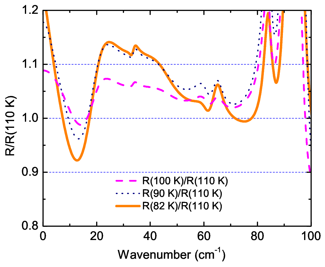
Figure 11: (color online) Calculated ratio of reflectance of the spectra below 110 K to the spectrum at 110 K.

The discussion in Section III puts in evidence a quite complex evolution of TTF-CA spectra with temperature. Such behavior is qualitatively reproduced by the calculation. An overall increase of reflectivity by lowering $T$ is brought in by the increase in $(\partial P/\partial\delta)^{2}$, and the shift of spectral weight towards lower frequency is accounted for by the change in the coupling constants $G_{j}$, as discussed after Eq. (4). However, we can gain a better insight into the factors affecting the temperature evolution of the spectra if better agreement between experiment and simulation is achieved. To such aim, Tab. 1 frequencies and coupling constants are used as starting values for a nonlinear fitting procedure based on Eqs. (2) and (4) to (7).

The variation of the frequencies and of the oscillator strengths with increasing $\varrho$ (lowering $T$) is induced in the model by the corresponding increase in both $\chi_{b}$ and $(\partial P/\partial\delta)^{2}$, as detailed in Table 2. However, it is clear from experiment that also the bandwidths (damping) $\Gamma_{j}$ change with $T$. In the model, the bandwidths are additional parameters, but in the fit we choose to correlate them to the anharmonicity introduced by the electron-phonon coupling. Following Fano,fano we impose the following relationship to $\Gamma_{j}$ (in cm^-1):

$$\Gamma_{j}=\mathtt{k}~{}~{}\frac{G_{j}^{2}}{\Omega_{j}}+2.0=\mathtt{k}~{}\eta_{j}+2.0.$$ (8)

On top of the intrinsic linewidth of 2.0 cm^-1, the electron-phonon coupling gives an additional contribution proportional to $\eta_{j}=G_{j}^{2}/\Omega_{j}$. The proportionality factor $\mathtt{k}$ adds just one extra adjustable parameter to the fit, and Eq. (8) represents a strong constrain. The fit shows a high sensitivity of spectra on the adjustable parameters. Thus a variation of the unperturbed frequencies $\omega_{i}$ or of the coupling constants $g_{i}$ by a few per cent, may profoundly alter the shape of the calculated spectra, especially in the case of the strongly coupled modes which cluster around $70-80$ cm^-1. For this reason, it is a challenge to obtain a satisfactory fit at all temperatures.

Fig. 10 illustrates the results of the fit of the reflectivity spectra at three temperatures. The fit is restricted to the spectral region below 150 cm^-1, so that the CT transition and its variation with temperaturejacobsen83 is simulated by $\epsilon_{\infty}$. Furthermore, we allow the frequencies $\omega_{i}$ to increase by a few wavenumber on lowering $T$, in order to simulate the usual hardening due to thermal contraction. The coupling constants and the proportionality factor for the damping, $\mathtt{k}$, are instead kept temperature independent.

Albeit not all details of the spectrum are precisely reproduced, the essential features are caught: By lowering the temperature the reflectivity increases, with a redistribution of the oscillator strengths and of the bandwidths as the spectral weight shifts towards lower frequencies. The downshift of spectral weight becomes more dramatic just before the phase transition. This is clearly demonstrated in Fig. 11, which resembles the experimental behavior reported in Fig. 3. The shift of the spectral weight is accompanied by an increase of the bandwidth of the $\nu_{1}$, lowest frequency phonon, which becomes overdamped around 100 K and below (Fig. 10). The experimentally observed overdamping of the $\nu_{1}$ phonon in Fig. 8 is then explained by the transfer of the entire electron-phonon coupling strength to this phonon just before the phase transition, with associated increase of anharmonicity.

VI Discussion and conclusions

In this paper we have presented temperature dependent polarized reflectivity spectra collected down to 5 cm^-1 for TTF-CA crystals above the NIT. A detailed theoretical analysis of the data has allowed us to offer the first direct identification of the Peierls softening mechanism.

An indirect experimental evidence of the softening of lattice vibrations in TTF-CA was offered by the occurrence of combination (two-phonon) bands in vibrational spectra collected in the region of the intramolecular vibrations (mid-IR).sidebands Several broad bands were found in IR spectra of TTF-CA that could not be assigned to fundamental modes. These bands, whose intensity increases on approaching NIT, are symmetrically located at the low and high frequency side of a Raman band assigned to a totally-symmetric molecular vibration. The two side-bands are then assigned to the sum and difference combinations of the totally-symmetric molecular vibration with a lattice phonon. The frequency of this lattice phonon lowers from about 70 cm^-1 to about 20 cm^-1 when going from room temperature to 81 K, as illustrated by the dots in fig. 12. In the light of the present work, indicating a multi-mode Peierls coupling, the soft-phonon inferred from the analysis of combination bands must correspond to an “effective” Peierls phonon, resulting from the weighted contribution of the several Peierls-coupled modes.

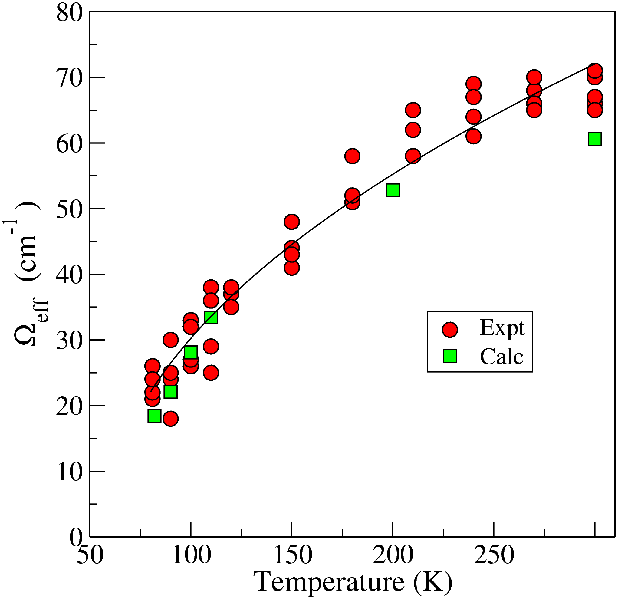
Figure 12: (color online) Experimental (taken from Ref. sidebands, ) and calculated frequency (squares) of the effective soft mode.

Specifically, the side-bands in the mid-IR region result from the combination of a totally symmetric molecular vibration with a superposition of several $B_{u}$ modes. Thus the apparent peak frequency of the effective soft mode, $\Omega_{\rm eff}$, is the weighted average of the frequencies of the Peierls phonons. In order to calculate $\Omega_{\rm eff}$ from the spectral simulation discussed in the previous Section, we adopt the following expression:

$$\Omega_{\rm eff}=\frac{\sum_{j}\eta_{j}\Omega_{j}}{\sum_{j}\eta_{j}},$$ (9)

where each frequency is weighted by $\eta_{j}$, the same factor entering the definition of vibrational linewidth in Eq. (8), and connected to the strength of the Peierls coupling. The computed value of $\Omega_{\rm eff}$ is compared with experiment in Fig. 12. The very good agreement between the effective phonon frequency obtained from the analysis of combination bands in the mid-IR region and of lattice phonons in the far-IR region strengthen our interpretation of the spectroscopic data in terms of a soft mode. Quite interestingly, the same effective soft mode of TTF-CA quantitatively accounts for the peaks observed in the diffuse X-ray scattering data.davino07

The softening of the lattice phonons, combined with the increase of their intensity on approaching NIT leads to very large vibrational contributions to the dielectric constant.freo02 ; soos04 By using the parameters found in the fit of reflectivity spectra, we can also estimate the temperature evolution of the static dielectric constant, $\epsilon_{1}$, which corresponds to the zero-frequency real part of the dielectric constant in Eq. 7. As shown in Fig. 13, the present estimate of $\epsilon_{1}$ agrees very well with available experimental data, strongly supporting the vibrational origin of the dielectric anomaly at NIT, as due to the large charge oscillations associated with the Peierls modes.freo02 ; soos04

Data analogous to the present ones have been previously reported Okimoto et al.,okimoto01 who discussed the reflectivity spectra along the stack of TTF-QBrCl₃ (QBrCl₃: 2-bromo-3,5,6-trichloro-$p$-benzoquinone), a CT crystal similar to TTF-CA that undergoes the NIT with continuous evolution of ionicity. However, in that work the reflectivity data have been collected only from 650 down to 25 cm^-1, so that the subsequent KKT transformation is delicate, and the discussion of conductivity spectra outside the experimentally accessed region should be taken with caution. In any case a broad band was enucleated from conductivity spectra which softens, without major broadening, from about 60 cm^-1 at 293 K to about 10 cm^-1 just above the critical temperature (71 K). This band was not ascribed to a soft mode, but rather to the pinned mode of the so-called neutral-ionic domain walls (NIDW).okimoto01 Whereas more extensive measurements are required to fully address this issue, our work on TTF-CA sheds doubts on this interpretation.

NIDWs were introduced theoretically by Nagaosa nagaosa86 as charged boundaries of I dimerized domains excited in the host N regular chain. Quite interestingly, they were originally restricted to the close proximity of discontinuous NIT, while the energy of the domains is often too large to allow for thermal population.soos07 However, NIDWs have been quite often invoked to explain the rich phenomenology of NIT.ricemem ; tokurareview In particular, the above mentioned dielectric anomaly and the combination bands in mid-IR spectra were initially attributed to NIDWs,IR-NIDW as well as the peak in the diffuse X-ray signal.buron06 As discussed above, this paper gives definitive support to a different picture that, without invoking exotic excitations, quantitatively explains the rich and variegated phenomenology of NIT to the increase of the effective Peierls coupling on approaching NIT. In this way different and apparently unrelated phenomena are all naturally and quantitatively explained in terms of the softening of lattice phonons coupled via a Peierls mechanism to delocalized electrons.

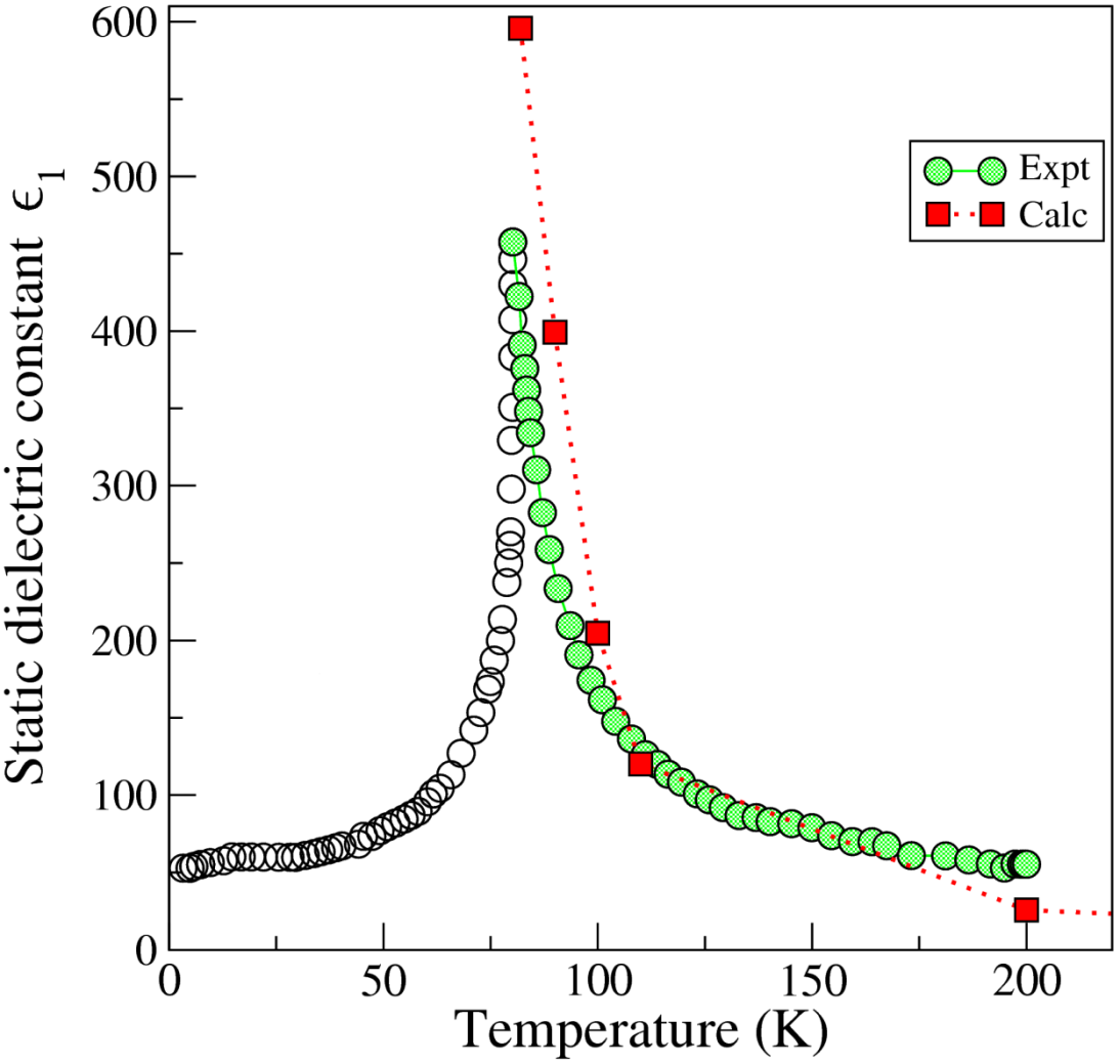
Figure 13: (color online) Experimental (taken from Ref. TTFCAdiel, ) and calculated [Eq. (7)] static dielectric constant of TTF-CA as a function of temperature.

The definitive and unambiguous support to the above picture is obtained by a careful analysis of the far-IR spectral region to directly identify the Peierls modes. The analysis is non-trivial: apart from the requirement for very refined experimental data extending down to very low-frequency, the spectral interpretation is based on a model for multi-mode Peierls coupling that combines lattice dynamics (QHLD) calculations with the modified Hubbard-model for the electronic structure. In fact, in the presence of several phonons the multi-mode Peierls softening is a complex phenomenon: the mode description changes on approaching the transition, with associated mode mixing, intensity redistribution and broadening. In the course of this mixing, the softening “jumps” from one mode to the nearest one below, until in the proximity of the phase transition all the softening is transferred to the lowest frequency mode. The mechanism, evident in the simulation presented in Fig. 9, explains the softening observed in Fig. 6 and the temperature behavior of mode intensities and linewidths in Fig. 7. The increase of the electronic susceptibility as the system is driven towards the NIT implies an increased effective coupling, and accordingly the spectral weight shifts towards zero frequency for $T<100$ K. Indeed, in this temperature range the Peierls coupling is almost completely transferred to the lowest-frequency mode. At the same time, the relevant bandwidth broadens, finally leading to an overdamped behavior. For this reason, in the spectra we just see the reflectivity increase towards zero frequency (Figs. 2 and 3), without being able to actually detect the full absorption. Overdamping has been often observed in ferroelectric phase transitions.nakamura66 In the case of TTF-CA, we are able to provide the microscopic origin of this effect.

VII Acknowledgments

The single crystals were kindly supplied by N. Karl (Universität Stuttgart). The work in Italy was supported by the Ministero Istruzione, Università e Ricerca (MIUR), through FIRB-RBNE01P4JF and   PRIN2004033197_002,   and in Stuttgart University by the Deutsche Forschungsgemeinschaft (DFG). N.D. thanks the Alexander von Humboldt foundation and the Scientific schools grant NSH-5596.2006.2 for the support.

References

- (1) R. E. Peierls,Quantum Theory of Solids (Oxford, Clarendon, 1955), p. 108.
- (2) H. M. McConnell and R. J. Lynden-Bell, J. Chem. Phys. 36, 2393 (1962); D. D. Thomas, H. J. Keller, and H. M. McConnell, J. Chem. Phys. 39, 2321 (1963).
- (3) J. W. Bray, L. V. Interrante, I. S. Jacobs, J. C. Bonner, Extended Linear Chain Compounds, Vol. 3, edited by J. S. Miller, (Plenum, New York, 1983).
- (4) J. B. Torrance, J. E. Vazquez, J. J. Mayerle, and V. Y. Lee, Phys. Rev. Lett. 46 (1981) 253.
- (5) J. B. Torrance, A. Girlando, J. J. Mayerle, J. I. Crowley, V. Y. Lee, P. Batail, and S. J. LaPlaca, Phys. Rev. Lett. 47 (1981) 1747.
- (6) A. Girlando and A. Painelli, Phys. Rev. B 34, 2131 (1986).
- (7) N. Nagaosa and J. Takimoto, J. Phys. Soc. Japan 55, 2737 (1986).
- (8) A. Girlando, A. Painelli, S. A. Bewick, and Z. G. Soos, Synth. Metals 141, 129 (2004).
- (9) S. Horiuchi, R. Kumai, Y. Okimoto, and Y. Tokura, Chem. Phys. 325, 78 (2006).
- (10) S. Horiuchi, Y. Okimoto, R. Kumai, and Y. Tokura, J. Phys. Soc. Jpn. 69, 1302 (2000).
- (11) M. Buron-Le Cointe, M. H. Lemee-Cailleau, H. Cailleau, S. Ravy, J. F. Berar, S. Rouziere, E. Elkaim, and E. Collet, Phys. Rev. Lett. 96, 205503 (2006).
- (12) L. Del Freo, A. Painelli, and Z. G. Soos, Phys. Rev. Lett. 89, 027401 (2002).
- (13) Z. G. Soos, S. A. Bewick, A. Peri, and A. Painelli, J. Chem. Phys. 120, 6712 (2004).
- (14) G. D’Avino, A. Girlando, A. Painelli, M. H. Lemée-Cailleau, and Z. G. Soos, Phys. Rev. Lett. 99, 156407 (2007).
- (15) Y. Tokura, S. Koshihara, Y. Iwasa, H. Okamoto, T. Komatsu, T. Koda, N. Iwasawa, and G. Saito, Phys. Rev. Lett. 63, 2405 (1989).
- (16) T. Nakamura, J. Phys. Soc. Japan 21, 491 (1966).
- (17) A. Moreac, A. Girard, Y. Dulugeard, and Y. Marqueton, J. Phys.: Condens. Matter 8, 3553 (1996).
- (18) Y. Okimoto, S. Horiuchi, E. Saitoh, R. Kumai, and Y. Tokura, Phys. Rev. Lett. 87, 187401 (2001).
- (19) M. Masino, A. Girlando, A. Brillante, R. G. Della Valle, E. Venuti, N. Drichko, and M. Dressel, Chem Phys. 325, 71 (2006).
- (20) M. Masino, A. Girlando, and Z. G. Soos, Chem. Phys. Lett. 369, 428 (2003).
- (21) C. C. Homes, M. Reedyk, D. A. Cradles, and T. Timusk, Applied Optics 32, 2976 (1993).
- (22) C. S. Jacobsen and J. B. Torrance, J. Chem. Phys. 78, 112 (1983).
- (23) A. Girlando, F. Marzola, C. Pecile, J. B. Torrance, J. Chem. Phys. 79, 1075 (1983).
- (24) A. Girlando and A. Painelli, J. Chem. Phys. 84, 5655 (1986); C. Pecile, A. Painelli, and A. Girlando, Mol. Cryst. Liq. Cryst. 171, 69 (1989).
- (25) A. Landrum and W. V. Glassey, “bind” (ver 3.0), distributed as part of the extended Hückel molecular orbital package (YaHEmop), freely available on the WWW at: http://sourceforge.net/projects/yaehmop/
- (26) M. Le Cointe, M. H. Lemée-Cailleau, H. Cailleau, B. Toudic, L. Toupet, G. Heger, F. Moussa, P. Schweiss, K. H. Kraft, and N. Karl, Phys. Rev. B 51, 3374 (1995).
- (27) A. Painelli and A. Girlando, Phys. Rev. B 37, 5748 (1988), and Phys. Rev. B 39, 9663 (1989).
- (28) U. Fano, Phys. Rev. 124, 1866 (1961).
- (29) Z. G. Soos and A. Painelli, Phys. Rev. B 75, 155119 (2007).
- (30) S. Horiuchi, Y. Okimoto, R. Kumai, and Y. Tokura, J. Phys. Soc. Japan 69, 1302 (2000), and J. Am. Chem. Soc. 123, 665 (2001).