Duality relation and joint measurement in a Mach-Zehnder Interferometer

Abstract

The Mach-Zehnder interferometric setup quantitatively characterizing the wave-particle duality implements in fact a joint measurement of two unsharp observables. We present a necessary and sufficient condition for such a pair of unsharp observables to be jointly measurable. The condition is shown to be equivalent to a duality inequality, which for the optimal strategy of extracting the which-path information is more stringent than the Jaeger-Shimony-Vaidman-Englert inequality.

I Introduction

Bohr’s principle of complementarity Bohr , a statement that a single quantum system possesses mutually exclusive but equally real properties, is an essential feature that distinguishes quantum from classical realm. The best-known manifestation of this principle is the wave-particle duality, i.e., the fact that a quantum object can at times behave as a wave and at other times behave as a particle, depending on the circumstances of the experiment being performed Scully . Since the pioneering work of Wootters and Zurek WZ , the conventional qualitative characterization of the wave-particle duality has acquired its quantitative version. In particular, in a two-path interferometer such as a Mach-Zehnder interferometer, there exist two kinds of trade-off relations between the fringe visibility of the interference pattern and the maximum amount of which-path information. The first one, known as uncertainty relationship for preparation, is about the trade-off between the a priori fringe visibility $\mathcal{V}_{0}$ of the interference pattern and the path predictability $\mathcal{P}$ GY ; Mandel . The measurements of $\mathcal{V}_{0}$ and $\mathcal{P}$ can only be carried out by two incompatible experimental setups since two noncommuting sharp observables must be measured. The second one is about the trade-off between the fringe visibility $\mathcal{V}$ and the path distinguishability $\mathcal{D}$ obtained simultaneously in a single experimental setup equipped with a which-path detector. Such a setup was first considered independently by Jaeger et al. Jaeger95 and Englert et al. Englert ; EnglertBergou . They established quantitative duality relations such as

$$\mathcal{D}^{2}+\frac{1-\mathcal{P}^{2}}{\mathcal{V}_{0}^{2}}\mathcal{V}^{2}\leq 1,$$ (1)

which we refer to as the Jaeger-Shimony-Vaidman-Englert inequality.

A second manifestation of quantum complementarity is the impossibility of jointly measuring some pairs of (sharp or unsharp) observables unsharp ; jm ; jm1 ; Busch ; BS . The Jaeger-Shimony-Vaidman-Englert setup implements in fact a joint measurement of two unsharp observables, i.e., a nonideal joint measurement of two noncommuting sharp observables. A fundamental question naturally arises: does the condition under which such two unsharp observables are jointly measurable dictate a duality relation? In this paper we answer this question in the positive. In Sec. II, we will give explicit expressions of two unsharp observables jointly measured in Englert’s setup Englert . Then, in Sec. III, we will derive a necessary and sufficient condition for such a pair of unsharp observables to be jointly measurable. In Sec. IV we will show that the condition is equivalent to a duality inequality characterizing the trade-off between the fringe visibility and the path distinguishability. One will see that the duality inequality is more stringent than the Jaeger-Shimony-Vaidman-Englert inequality for the optimal strategy of extracting the which-path information. We conclude with some discussions in Sec. V.

II Two unsharp observables jointly measured in Englert’s setup

A standard Mach-Zehnder interferometer as considered by Englert Englert can be described by a two-dimensional Hilbert space spanned by two orthonormal states $|0\rangle$ and $|1\rangle$ representing two distinct paths (see Fig. 1). A generic state of the quanton prior to entering the interferometer can be represented by a density operator $\rho$ on this two-dimensional Hilbert space. After passing a beam splitter which, without loss of generality, is described by the Hadamard transformation $H=(\sigma_{x}+\sigma_{z})/\sqrt{2}$, the quanton undergoes a phase shifter $\Phi=e^{i\phi\sigma_{z}/2}$, and then the two beams are combined on another beam splitter which is also described by the Hadamard transformation.

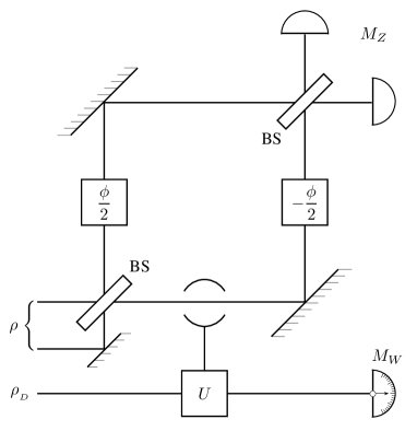
Figure 1: The schematic sketch of a Mach-Zehnder interferometer with a which-path detector. The quanton undergoes a projective measurement $M_{Z}$ of $\sigma_{z}$ after it has passed through the second beam splitter, and the detector undergoes a projective measurement $M_{W}$ of $\hat{W}$.

Immediately follows from the positivity of the density matrix a quantitative duality relation $\mathcal{P}^{2}+\mathcal{V}_{0}^{2}\leq 1$ between the a priori fringe visibility $\mathcal{V}_{0}=2\left|\langle+|\rho|-\rangle\right|$ and the predictability $\mathcal{P}=\left|w_{+}-w_{-}\right|$ with $w_{\pm}=\langle\pm|\rho|\pm\rangle$ being the probabilities for the quanton taking the two paths respectively, where $|\pm\rangle=(|0\rangle\pm|1\rangle)/\sqrt{2}$ are two eigenvectors of $\sigma_{x}.$ To test this duality relation, two projective measurements must be made: $\sigma_{x}$ for the predictability $\mathcal{P}=|\langle\sigma_{x}\rangle_{\rho}|$ and

$$\sigma_{\phi}=(H\Phi H)^{\dagger}\sigma_{z}(H\Phi H)=\sigma_{z}\cos\phi-\sigma_{y}\sin\phi$$ (2)

for the a priori fringe visibility

$$\mathcal{V}_{0}=\max_{\phi}\langle\sigma_{\phi}\rangle_{\rho},$$ (3)

the maximum being attained when $\phi$ is set to be the phase factor $\phi_{0}$ of $\langle-|\rho|+\rangle$. Note that $\sigma_{x}$ and $\sigma_{\phi_{0}}$ are a pair of noncommuting sharp observables, whose measurements cannot be fulfilled in a single experimental setup.

To simultaneously obtain the which-path information and the interference pattern, a detector is coupled with the quanton by a controlled unitary transformation $U_{QD}=|0\rangle\langle 0|\otimes I_{D}+|1\rangle\langle 1|\otimes U$ after the quanton passes through the first beam splitter, where $I_{D}$ and $U$ are respectively the identity operator and a unitary operator on the Hilbert space of the detector. The fringe visibility $\mathcal{V}=\mathcal{V}_{0}\left|\mathrm{tr}_{D}\left(U\rho_{D}\right)\right|$ is evidently smaller than the a priori fringe visibility, where $\rho_{D}$ is the initial state of the detector. However, the measurement of an observable $\hat{W}$ of the detector can be exploited to increase our knowledge about the which-path information.

A general strategy $\mathcal{S}$ of extracting the which-path information is to split all the outcomes $W$ of measuring the observable $\hat{W}$ into two disjoint sets $S$ and $\bar{S}$: if $W\in S$ then we guess that the quanton takes path $|0\rangle$ and if $W\in\bar{S}$ then we guess that the quanton takes path $|1\rangle$. By denoting

$$\eta_{S}=\sum_{W\in S}\langle W|\rho_{D}|W\rangle,\;\eta_{S}^{U}=\sum_{W\in S}\langle W|U\rho_{D}U^{\dagger}|W\rangle,$$ (4)

and similarly for $\bar{S},$ the “likelihood for guessing the path right” is then given by $(1+\mathcal{D}_{\mathcal{S}})/2$, where

$$\mathcal{D}_{\mathcal{S}}\equiv 2w_{+}\eta_{S}+2w_{-}\eta_{\bar{S}}^{U}-1$$ (5)

is the path distinguishability. By further choosing $\hat{W}$ to be such that its eigenvectors $|W\rangle$ are also eigenvectors of $w_{+}\rho_{D}-w_{-}U\rho_{D}U^{\dagger}$ and splitting the outcomes $W$ according to

$$W\in\left\{\begin{array}[]{ccc}S,&&\text{if }\langle W|w_{+}\rho_{D}|W\rangle>\langle W|w_{-}U\rho_{D}U^{\dagger}|W\rangle\\ \bar{S},&&\text{if }\langle W|w_{+}\rho_{D}|W\rangle<\langle W|w_{-}U\rho_{D}U^{\dagger}|W\rangle\end{array}\right.,$$ (6)

the path distinguishability attains its maximum

$$\mathcal{D}=\mathrm{tr}_{D}\left|w_{+}\rho_{D}-w_{-}U\rho_{D}U^{\dagger}\right|.$$ (7)

By use of this mathematical expression of $\mathcal{D}$, Englert succeeded in proving the Jaeger-Shimony-Vaidman-Englert inequality in Eq. (1).

In the following we shall identify two unsharp observables that are jointly measured in the above experimental setup, or two noncommuting sharp observables jointly measured in a nonideal way. The first unsharp observable is described by the positive-operator-valued measure (POVM) $\mathcal{N}=\{N_{0},N_{1}\},$ where

$$N_{0}=\frac{1}{2}\left(I+\frac{\mathcal{V}}{\mathcal{V}_{0}}\sigma_{\delta+\phi}\right)=I-N_{1}$$ (8)

with $\delta$ being the phase of $\mathrm{tr}_{D}(\rho_{D}U^{\dagger})$. It is obviously a smeared version of the sharp observable $\sigma_{\delta+\phi}.$ The probability of the quanton emerging from the output port $i$ ($i=0,1$) is $\mathrm{tr}_{Q}(\rho N_{i})$. Similar to Eq. (3), the fringe visibility in this case can be written as

$$\mathcal{V}=\max_{\phi}(\langle N_{0}\rangle_{\rho}-\langle N_{1}\rangle_{\rho}),$$ (9)

the maximum being attained when $\delta+\phi=\phi_{0}$.

The second unsharp observable, a smeared version of the sharp observable $\sigma_{x}$, is described by the POVM $\mathcal{M}=\{M_{0},M_{1}\},$ where

$$M_{0}=\frac{\eta_{S}+\eta_{S}^{U}}{2}I+\frac{\eta_{S}-\eta_{S}^{U}}{2}\sigma_{x}=I-M_{1}.$$ (10)

The probability of finding the detector in a state belonging to $S$ (or $\bar{S}$) is $\mathrm{tr}_{Q}(\rho M_{0})$ [or $\mathrm{tr}_{Q}(\rho M_{1})$].

In fact, the setup implements a measurement of a bivariate four-outcome observable $\{E_{ij}{,\;i,j=0,1}\}$ where

$$E_{i0}=\sum_{W\in S}E_{iW},\quad E_{i1}=\sum_{W\in\bar{S}}E_{iW},$$ (11)

together with

$$E_{iW} = \mathrm{tr}_{D}[(I\otimes\rho_{D})\mathcal{U}^{\dagger}(|i\rangle\langle i|\otimes|W\rangle\langle W|)\mathcal{U}],$$

$$\mathcal{U} = (H\otimes I)U_{QD}(\Phi H\otimes I).$$

The $E_{ij}$’s satisfy the following two identities

$$\sum_{j=0,1}E_{ij}=N_{i},\quad\sum_{i=0,1}E_{ij}=M_{j},$$ (12)

so that recording the result $i$ is a measurement of the observable $\mathcal{N}$, while recording the result $j$ is a measurement of the observable $\mathcal{M}$. In general, two unsharp observables $\mathcal{N}$ and $\mathcal{M}$ are jointly measurable if and only if there exists a single experimental setup measuring a bivariate “joint observable” $\{E_{ij}\}$ whose marginals are $\mathcal{N}$ and $\mathcal{M}$ jm ; jm1 ; Busch ; BS .

III Necessary and sufficient condition for joint measurability

The unsharp observables of interest here are of the following kinds

$$N_{0} = \frac{I}{2}+\bm{n}\cdot\bm{\sigma}=I-N_{1},$$

$$M_{0} = m_{0}I+\bm{m}\cdot\bm{\sigma}=I-M_{1}$$ (13)

with ${\bm{n}\cdot\bm{m}}=0.$ Now, what is the criterion for such a pair of unsharp observables to be jointly measurable? Only in the special case where $m_{0}=1/2$ did Busch offer the answer to this question Busch . But in the case of a general $m_{0}$, this is an open question so far. Here, we establish the following theorem:

Theorem 1. Two unsharp observables $\mathcal{N}$ and $\mathcal{M}$ as given in Eq. (13) are jointly measurable if and only if

$$\sqrt{m_{0}^{2}-m^{2}}+\sqrt{(1-m_{0})^{2}-m^{2}}\geq 2n,$$ (14)

where $m=|{\bm{m}}|$ and $n=|{\bm{n}}|.$

Proof. The most general forms of ${E_{ij}}$’s that take the $N_{i}$’s and the $M_{j}$’s as marginals [i.e., that satisfy Eq. (12)] read as

$$E_{ij}=x_{ij}I+\bm{y}_{ij}\cdot\bm{\sigma}$$

with

$$x_{ij} = \tfrac{1}{4}+\tfrac{1}{4}(-)^{j}(2m_{0}-1)+(-)^{i+j}\tfrac{1}{2}x,$$

$$\bm{y}_{ij} = \tfrac{1}{2}\left[(-)^{j}\bm{m}+(-)^{i}\bm{n}+(-)^{i+j}\bm{y}\right],$$

where $x$ is a real number and $\bm{y}$ is a vector in the three-dimensional Euclidean space $\mathbb{R}^{3}$. The positivity of the $E_{ij}$’s entails the conditions $x_{ij}\geq\left|\bm{y}_{ij}\right|$ for all $i,j$. Therefore the joint measurability of $\mathcal{N}$ and $\mathcal{M}$ is equivalent to the existence of $x$ and $\bm{y}$ such that

$$\left|\bm{m}+\bm{n}+\bm{y}\right| \leq m_{0}+x,\quad\left|\bm{m}-\bm{n}+\bm{y}\right|\leq 1-m_{0}-x,$$

$$\left|\bm{m}-\bm{n}-\bm{y}\right| \leq m_{0}-x,\quad\left|\bm{m}+\bm{n}-\bm{y}\right|\leq 1-m_{0}+x.$$

Sufficiency. If the inequality Eq. (14) holds then the choice $x=0$ and $\bm{y}=y\bm{n}/n$ with

$$y=\min\Big{\{}\sqrt{m_{0}^{2}-m^{2}}-n,n+\sqrt{(1-m_{0})^{2}-m^{2}}\Big{\}}$$ (16)

will make all four inequalities in Eq. (LABEL:ineq) hold. Hence a joint observable can be explicitly constructed and the two unsharp observables $\mathcal{N}$ and $\mathcal{M}$ are joint measurable.

Necessity. Let us denote by $\mathcal{P}_{\bm{mn}}$ the plane spanned by $\bm{m}$ and $\bm{n}$ in $\mathbb{R}^{3}$ (see Fig. 2). A point $Y$ in $\mathbb{R}^{3}$ corresponds to a vector $\bm{y}\$whose initial point is the original point $O$ and whose end point is $Y,$ so when we say “a point $\bm{y}$” we mean the corresponding vector. The four points $A,$ $B,$ $C,$ and $D$ correspond to the vectors $-\bm{n}+\bm{m},$ $\bm{m}+\bm{n},$ $\bm{-m-n},$ and $\bm{n}-\bm{m},$ respectively. The four points $P,$ $Q,$ $S,$ and $T$ denote midpoints of the line segments $AC,$ $BD,$ $AB,$ and $CD$, respectively. The first inequality in Eq. (LABEL:ineq) means that the distance between the points $\bm{-m-n}$ and $\bm{y}$ is bounded by $m_{0}+x,$ and similarly for the other three inequalities.

Suppose that the two unsharp observables $\mathcal{N}$ and $\mathcal{M}$ are jointly measurable. Then there exist $x$ and $\bm{y}$ satisfying all four inequalities in Eq. (LABEL:ineq). If $\bm{y}\notin\mathcal{P}_{\bm{mn}}$, then there must be a new point, e.g., the orthogonal projector $\bm{y}^{\prime\prime}$ of $\bm{y}$ onto $\mathcal{P}_{\bm{mn}},$ that also satisfies the four inequalities in Eq. (LABEL:ineq) with the same $x$. Further, if $\bm{y}^{\prime\prime}=\overrightarrow{OY^{\prime\prime}},$ with $Y^{\prime\prime}$ being outside the rectangle $ABCD$ (see Fig. 2), then there must be a new point inside the rectangle that also satisfies the four inequalities in Eq. (LABEL:ineq) with the same $x$. To see this, let $E$ denote the orthogonal projection of $Y^{\prime\prime}$ onto the sideline $BD,$ and let $Y^{\prime}\in\square ABCD$ denote a point on the extension line of $Y^{\prime\prime}E$ satisfying $Y^{\prime}E\leq Y^{\prime\prime}E$. It is evident that $AY^{\prime}<AY^{\prime\prime},$ $BY^{\prime}\leq BY^{\prime\prime},$ $CY^{\prime}<CY^{\prime\prime},$ and $DY^{\prime}\leq DY^{\prime\prime}$, so the vector $\bm{y}^{\prime}=\overrightarrow{OY^{\prime}}$ together with the same $x$ also satisfies the four inequalities in Eq. (LABEL:ineq).

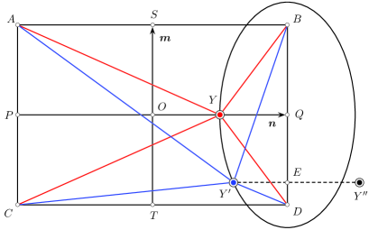
Figure 2: Illustration of the fact that joint measurability of the two unsharp observables $\mathcal{N}$ and $\mathcal{M}$ ensures the existence of a point belonging to the line segment $PQ$ such that the corresponding vector satisfies the four inequalities in Eq. (LABEL:ineq) together with $x=0$.

Then we will show that if $x$ and $\bm{y}^{\prime}\in\square ABCD$ satisfy the four inequalities in Eq. (LABEL:ineq), then there must be a point belonging to the line segment $PQ$ which satisfies the four inequalities in Eq. (LABEL:ineq) together with $x=0$. For the moment we will consider the case $Y^{\prime}\in\square OQTD$ (see Fig. 2) and $x\geq 0$. Other cases can be proved similarly. Let us denote by $\mathcal{E}_{BDY^{\prime}}$ the ellipse whose foci are $B$ and $D$ and which passes through the point $Y^{\prime}$, and denote by $Y$ the point of intersection of the ellipse with the straight line $PQ$. The point $Y$ may lie inside the line segment $PQ$ or outside. For the moment we assume that it is inside the line segment $PQ$. By assumption, we have

$$AY^{\prime} \leq m_{0}-x,\quad BY^{\prime}\leq 1-m_{0}+x,$$

$$CY^{\prime} \leq m_{0}+x,\quad DY^{\prime}\leq 1-m_{0}-x.$$

First, observe that

$$CY=AY\leq AY^{\prime}\leq m_{0}-x\leq m_{0}.$$

Then, let $\Delta$ be the difference between $BY^{\prime}$ and $BY$: $BY^{\prime}-BY=\Delta.$ Due to the property of an ellipse, we also have $DY-DY^{\prime}=\Delta.$ If $\Delta\geq x,$ then we have

$$DY=BY=BY^{\prime}-\Delta\leq 1-m_{0}+x-\Delta\leq 1-m_{0}.$$

If $\Delta\leq x,$ then we have

$$BY=DY=DY^{\prime}+\Delta\leq 1-m_{0}-x+\Delta\leq 1-m_{0}.$$

So $\overrightarrow{OY}$ is a vector that satisfies Eq. (LABEL:ineq) together with $x=0$.

If $Y$ is outside $PQ$, i.e., if it lies on the left of $P$, then following the similar way one can show that $\overrightarrow{OP}$ satisfies the four inequalities in Eq. (LABEL:ineq) together with $x=0$.

Similar arguments apply to the cases of $Y^{\prime}\notin\square OQTD$, but in some cases we need to consider the ellipse $\mathcal{E}_{ACY^{\prime}}$ whose foci are $A$ and $C$ and which passes through the point $Y^{\prime}$. We summarize that in the cases $\{x\geq 0,\;Y^{\prime}\in\square PQDC\}$ and $\{x\leq 0,\;Y^{\prime}\in\square ABQP\}$ one should consider the ellipse $\mathcal{E}_{BDY^{\prime}},$ while in the cases $\{x\leq 0,\;Y^{\prime}\in\square PQDC\}$ and $\{x\geq 0,\;Y^{\prime}\in\square ABQP\}$ one should consider the ellipse $\mathcal{E}_{ACY^{\prime}}.$

To sum up, a necessary condition for the two unsharp observables $\mathcal{N}$ and $\mathcal{M}$ to be jointly measurable is the existence of a number $y\in[-n,n]$ such that

$$m^{2}+(n+y)^{2}\leq m_{0}^{2},\quad m^{2}+(n-y)^{2}\leq(1-m_{0})^{2},$$ (17)

from which the inequality in Eq. (14) immediately follows. $\square$

IV Duality relation from joint measurability

In Sec. II we have seen that to each strategy $\mathcal{S}$ there correspond two unsharp observables $\mathcal{N}$ and $\mathcal{M}$ with

$$\bm{n} = \frac{\mathcal{V}}{2\mathcal{V}_{0}}(0,\;-\sin{\phi_{0}},\;\cos{\phi_{0}}),$$

$$m_{0} = \frac{\eta_{S}+\eta_{S}^{U}}{2},$$

$$\bm{m} = \frac{\eta_{S}-\eta_{S}^{U}}{2}(1,\;0,\;0).$$

Theorem 1 states that their joint measurability entails a bound on $\mathcal{V}/\mathcal{V}_{0}$:

$$\frac{\mathcal{V}}{\mathcal{V}_{0}}\leq\sqrt{\eta_{S}\eta_{S}^{U}}+\sqrt{\eta_{\bar{S}}\eta_{\bar{S}}^{U}}.$$ (18)

In the following we will show that this joint measurability condition is equivalent to a duality inequality.

From the definition Eq. (5) of the path distinguishability $\mathcal{D}_{\mathcal{S}}$ of a given strategy $\mathcal{S}$ and the identities $\eta_{S}+\eta_{\bar{S}}=1,$ $\eta_{S}^{U}+\eta_{\bar{S}}^{U}=1,$ and $w_{+}+w_{-}=1,$ we obtain the following identity

$$\mathcal{D}_{\mathcal{S}}^{2}+\left(\sqrt{\eta_{S}\eta_{S}^{U}}+\sqrt{\eta_{\bar{S}}\eta_{\bar{S}}^{U}}\right)^{2}(1-\mathcal{P}^{2})=1-\gamma_{\mathcal{S}}^{2},$$

where

$$\gamma_{\mathcal{S}}=2\Big{|}w_{+}\sqrt{\eta_{S}\eta_{\bar{S}}}-w_{-}\sqrt{\eta_{S}^{U}\eta_{\bar{S}}^{U}}\,\Big{|}.$$

This identity together with the inequality in Eq. (18) leads us to our main theorem:

Theorem 2. When a general strategy $\mathcal{S}$ of extracting the which-path information is adopted, the joint measurability condition of the two unsharp observables $\mathcal{N}$ and $\mathcal{M}$ is equivalent to the following duality inequality characterizing the trade-off between the fringe visibility and the path distinguishability:

$$\mathcal{D}_{\mathcal{S}}^{2}+\frac{1-\mathcal{P}^{2}}{\mathcal{V}_{0}^{2}}\mathcal{V}^{2}\leq 1-\gamma_{\mathcal{S}}^{2}.$$ (19)

Notice that this duality inequality is for a general strategy $\mathcal{S}$ and our derivation has not invoked the mathematical expression of the optimal distinguishability $\mathcal{D}$, in sharp contrast to Englert’s derivation of the Jaeger-Shimony-Vaidman-Englert inequality. When we adopt the optimal strategy $\mathcal{S}_{\mathrm{opt}}$ for extracting the which-path information, i.e., when $\mathcal{D}_{\mathcal{S}}$ attains its maximum $\mathcal{D}$, the Jaeger-Shimony-Vaidman-Englert inequality follows immediately from our duality inequality. Although $\gamma_{\mathcal{S}_{\mathrm{opt}}}$ does vanish for a pure $\rho_{D}$ (which will be proved in Appendix, Sec. A.1), our duality inequality is more stringent since $\gamma_{\mathcal{S}_{\mathrm{opt}}}$ does not generally vanish. For example, if we take the detector to be a two-dimensional system and let $w_{+}=(1+p)/2$ with $p$ being small then we have

$$\gamma_{\mathcal{S}_{\mathrm{opt}}}\approx\frac{2(1-\mathrm{tr}\rho_{D}^{2})}{F(\rho_{D},U\rho_{D}U^{\dagger})}|p|+o(p^{2})$$ (20)

with $F$ being the quantum fidelity. It is clear that $\gamma_{\mathcal{S}_{\mathrm{opt}}}$ in this case does not vanish for any mixed $\rho_{D}$. See Appendix, Sec. A.2 for a proof of Eq. (20).

V Conclusions and discussions

We have derived the necessary and sufficient condition for joint measurability of two unsharp observables of the form in Eq. (13). This is a substantial step towards solving the long-standing joint measurability problem—given two unsharp observables, are they jointly measurable? In fact, few such steps have ever been taken in the past two decades, since the precursory work by Busch Busch . We have also shown that our joint measurability condition is equivalent to a duality relation between the fringe visibility and the path distinguishability in Englert’s setup, thus establishing an intimate relationship between two different manifestations of quantum complementarity.

Although our duality inequality is more stringent than the Jaeger-Shimony-Vaidman-Englert inequality due to the quantity $\gamma_{\mathcal{S}}^{2}$ in Eq. (19), we do not have a physical interpretation of the quantity at present. In the past few years there have appeared other duality inequalities different from the Jaeger-Shimony-Vaidman-Englert kind. To take just one example, Jakob and Bergou JakobBergou established an intriguing inequality between the local properties visibility and predictability and the nonlocal property concurrence which is a quantitative entanglement measure. The relationship between these duality inequalities and ours is yet unclear.

Another two open questions deserve further research. 1) The setup we considered in this paper obviously simultaneously measures not merely two unsharp observables $\mathcal{N}$ and $\mathcal{M},$ but three: $\mathcal{N}$, $\mathcal{M}$, and $\{E_{00}+E_{11},E_{01}+E_{10}\}.$ One can expect that, although our present formalism (attached to two observables) is enough for disclosing the relationship between joint measurability and the duality relation, the condition for the above three unsharp observables to be jointly measurable will likely be tighter than that obtained in our present work, and so will likely lead to a tighter duality inequality. However, a simple single-inequality joint measurability condition for the three observables is unavailable so far. 2) One might wonder whether we can follow our way to derive a duality relation in a scenario more general than Englert’s. Although we have achieved a single-inequality joint measurability condition for two general unsharp qubit observables Sixia , and we have succeeded in transforming the condition to a duality relation [Eq. (6) of Ref. Sixia ] in some more general scenarios, but we have failed in doing so in the most general scenarios.

Note added. Recently, several works Sixia ; buschnew ; Heinosaari1 ; Heinosaari ; Brougham ; Busch08 ; stano have appeared on the topic of joint measurement of unsharp observables. For example, Busch and Heinosaari buschnew employed the notion of approximate joint measurement (in some reasonable sense) to present some necessary (but not sufficient) and some sufficient (but not necessary) conditions for two unsharp qubit observables to be jointly measurable. Remarkably, the joint measurability problem for two general unsharp qubit observables has been solved by three independent groups Sixia ; Busch08 ; stano . Yu et al. Sixia presented a single-inequality necessary and sufficient condition for joint measurability and proved the equivalence between the conditions formulated by the three groups.

Appendix

In this appendix, we present the proofs of some properties of $\gamma_{\mathcal{S}_{\mathrm{opt}}}.$

A.1 Quantity $\gamma_{\mathcal{S}_{\mathrm{opt}}}$ vanishes when $\rho_{D}$ is pure

Since both $\rho_{D}$ and $\rho_{D}^{U}$ are pure, we can restrict ourselves to the two-dimensional subspace spanned by these two pure states, and we can denote them in terms of the Pauli operators acting on the subspace:

$$\rho_{D}=\frac{I+\bm{\alpha}\cdot\bm{\sigma}}{2},\quad U\rho_{D}U^{\dagger}=\frac{I+\bm{\beta}\cdot\bm{\sigma}}{2},$$ (1)

where $\bm{\alpha}$ and $\bm{\beta}$ are unit vectors in $\mathbb{R}^{3}.$ The optimal strategy for extracting the which-path information is represented by the projective measurement $\{P_{\pm}\}$

$$P_{\pm}=\frac{I\pm\bm{s}\cdot\bm{\sigma}}{2},\quad\bm{s}=\frac{w_{+}\bm{\alpha}-w_{-}\bm{\beta}}{|w_{+}\bm{\alpha}-w_{-}\bm{\beta}|}$$ (2)

together with

$$\eta_{S}=\frac{1+\bm{\alpha}\cdot\bm{s}}{2},\quad\eta_{S}^{U}=\frac{1+\bm{\beta}\cdot\bm{s}}{2}.$$ (3)

Straightforward algebra gives

$$w_{+}^{2}\eta_{S}\eta_{\bar{S}}-w_{-}^{2}\eta_{S}^{U}\eta_{\bar{S}}^{U}=\frac{1-\mathrm{tr}\rho_{D}^{2}}{2}p.$$ (4)

Since $\rho_{D}$ is pure, we have $\mathrm{tr}\rho_{D}^{2}=1$ so that $w_{+}^{2}\eta_{S}\eta_{\bar{S}}-w_{-}^{2}\eta_{S}^{U}\eta_{\bar{S}}^{U}=0,$ i.e., $\gamma_{\mathcal{S}_{\mathrm{opt}}}=0.$

A.2 Proof of Eq. (20)

Suppose states $\rho_{D}$ and $\rho_{D}^{U}$ of the detector (a two-dimensional system) are of the form in Eq. (1) so that the optimal strategy is given by Eqs. (2) and (3). For convenience, let us denote $|\bm{\alpha}|^{2}=|\bm{\beta}|^{2}:=a$ and $\bm{\alpha}\cdot\bm{\beta}:=b.$ Since $\rho_{D}$ is a mixed state we have $a<1.$

The quantity $\gamma_{\mathcal{S}}$ can be rewritten as

$$\gamma_{\mathcal{S}}=2\frac{\left|w_{+}^{2}\eta_{S}\eta_{\bar{S}}-w_{-}^{2}\eta_{S}^{U}\eta_{\bar{S}}^{U}\right|}{w_{+}\sqrt{\eta_{S}\eta_{\bar{S}}}+w_{-}\sqrt{\eta_{S}^{U}\eta_{\bar{S}}^{U}}}.$$ (5)

Using the fact that $p$ is small we obtain

$$\frac{1}{w_{+}\sqrt{\eta_{S}\eta_{\bar{S}}}+w_{-}\sqrt{\eta_{S}^{U}\eta_{\bar{S}}^{U}}}=\frac{2}{\sqrt{1-\dfrac{a-b}{2}}}+o(p).$$ (6)

On the other hand, the identity

$$F(\rho_{D},U\rho_{D}U^{\dagger})=\sqrt{\mathrm{tr}(\rho_{D}U\rho_{D}U^{\dagger})+2\det\rho_{D}}$$ (7)

together with

$$\mathrm{tr}(\rho_{D}U\rho_{D}U^{\dagger})=\frac{1+b}{2},\quad\det\rho_{D}=\frac{1-a}{4}$$ (8)

leads to

$$F(\rho_{D},U\rho_{D}U^{\dagger})=\sqrt{1-\frac{a-b}{2}}.$$ (9)

It follows from Eqs. (6) and (9) that

$$\frac{1}{w_{+}\sqrt{\eta_{S}\eta_{\bar{S}}}+w_{-}\sqrt{\eta_{S}^{U}\eta_{\bar{S}}^{U}}}=\frac{2}{F(\rho_{D},U\rho_{D}U^{\dagger})}+o(p).$$ (10)

Finally, inserting Eqs. (4) and (10) into Eq. (5) gives Eq. (20), thus completing the proof.

References

• (1) N. Bohr, Naturwiss. 16, 245 (1928); Nature (London) 121, 580 (1928).
• (2) M. O. Scully, B.-G. Englert, and H. Walther, Nature (London) 351, 111 (1991).
• (3) W. K. Wootters and W. H. Zurek, Phys. Rev. D 19, 473 (1979).
• (4) D. M. Greenberger and A. Yasin, Phys. Lett. A 128, 391 (1988).
• (5) L. Mandel, Opt. Lett. 16, 1882 (1991).
• (6) G. Jaeger, A. Shimony, and L. Vaidman, Phys. Rev. A 51, 54 (1995).
• (7) B.-G. Englert, Phys. Rev. Lett. 77, 2154 (1996).
• (8) B.-G. Englert and J. A. Bergou, Opt. Commun. 179, 337 (2000).
• (9) Observables in terms of projection-valued measures are called to be sharp, while observables in terms of positive-operator-valued measures are called to be unsharp.
• (10) H. Martens and W. M. de Muynck, Found. Phys. 20, 255 (1990).
• (11) W. M. de Muynck, Foundations of Quantum Mechanics: An Empiricist Approach (Kluwer Academic Publishers, Dordrecht, 2002).
• (12) P. Busch, Phys. Rev. D 33, 2253 (1986).
• (13) P. Busch and C. Shilladay, Phys. Rep. 435, 1 (2006).
• (14) M. Jakob and J. A. Bergou, e-print arXiv:quant-ph/0302075.
• (15) S. Yu, N.-L. Liu, L. Li, and C. H. Oh, e-print arXiv:0805.1538.
• (16) P. Busch and T. Heinosaari, Quantum Inf. Comput. 8, 797 (2008).
• (17) T. Heinosaari, P. Stano, and D. Reitzner, Int. J. Quantum Inf. 6, 975 (2008).
• (18) T. Heinosaari, D. Reitzner, and P. Stano, Found. Phys. 38, 1133 (2008).
• (19) T. Brougham, E. Andersson, and S. M Barnett, e-print arXiv:0812.1474.
• (20) P. Busch and H.-J. Schmidt, e-print arXiv:0802.4167.
• (21) P. Stano, D. Reitzner, and T. Heinosaari, Phys. Rev. A 78, 012315 (2008).