Quantum model for double ionization of atoms in strong laser fields

Abstract

We discuss double ionization of atoms in strong laser pulses using a reduced dimensionality model. Following the insights obtained from an analysis of the classical mechanics of the process, we confine each electron to move along the lines that point towards the two-particle Stark saddle in the presence of a field. The resulting effective two dimensional model is similar to the aligned electron model, but it enables correlated escape of electrons with equal momenta, as observed experimentally. The time-dependent solution of the Schrödinger equation allows us to discuss in detail the time dynamics of the ionization process, the formation of electronic wave packets and the development of the momentum distribution of the outgoing electrons. In particular, we are able to identify the rescattering process, simultaneous direct double ionization during the same field cycle, as well as other double ionization processes. We also use the model to study the phase dependence of the ionization process.

I Introduction

Extensive experimental and theoretical studies of multiple ionization in strong laser fields have revealed a number of unexpected features. While some phenomena can be described as multi-photon, independent electron processes, (see e.g. gelt88 ), others require electron-electron correlations. This was concluded on the basis of a detailed analysis of experimental data together with precise calculations of single ionization rates anne82 ; review . Several experiments walker94 then revealed a pronounced “knee” structure in the yield vs peak laser intensity, typically plotted with logarithmic axis because of the wide range of values covered. Further ingenious experiments that resolved the joint momentum distributions of the outgoing electrons then showed that they often leave the atom with the same momenta review ; weber00n . This has triggered a number of theoretical studies of this process, including $S$-matrix calculations for the full cross sections becker00kopold00 , and investigations of simplified classical and quantum models. Among the models are so-called aligned-electron models aligned ; engel , in which electrons move in a one-dimensional (1D) regularized Coulomb potential, or quasi three-dimensional (3D) ones with the center of mass of the electrons confined to move along the field polarization axis becker . On the other hand, an exact solution of the time-dependent Schrödinger equation for two electrons in a laser field remains a formidable task, accessible usually to very short pulses of wavelengths shorter than 800 nm taylor ; parker06 .

One of the keys to understanding the dynamics of double and higher multiple-ionization is the rescattering scenario corkum93 . Most of the electrons escaping from the atom when the field is strong, leave definitely and contribute to the single ionization channel. Some, however, have their paths reversed back to the ionic core when the field changes sign. These electrons are then accelerated by the field and can share their energy with one or more electrons close to the nucleus. When they return to the ion, the electrons form a transient, short lived compound state which has several possible channels to decay: it can exit in a single ionization event, a double ionization event or a repetition of the rescattering cycle. Interestingly, starting from this intermediate situation, a classical analysis easily yields possible pathways to ionization and the effective potential eckhardt01pra1 . The classical analysis of double ionization suggests that the electrons may escape simultaneously if they pass sufficiently symmetrically over saddles that form in the presence of the electric field. As the field phase changes, the saddles move along lines that keep a constant angle with respect to the polarization axis eckhardt01pra1 .

The observation about the location of the saddles then suggested a way to reduce the degrees of freedom but to allow the possibility for the two electrons to escape with the same momentumeckhardt06 : as in the aligned electron models, the electrons are confined to move along lines, except that the lines pass through the location of the saddles and have an angle of $\pi/6$ with respect to the field axis. As other 1D+1D models, also this one allows to reproduce prauzner07 tunnelling and rescattering processes, single and sequential double ionizations but, in addition, it allows for escape with the same momentum and hence can mimic the correlated electron escape. In the aligned–electron model this process is suppressed by the overestimated Coulomb repulsion.

The aim of the present paper is to present the quantum version of this model and to discuss in detail its predictions for the ionization signal. Results for longer pulses have been described briefly before prauzner07 . The model is introduced and motivated in section II. Section III then contains technical information on numerical aspects of the calculations. Except for section III.2 on the methods used to distinguish the different ionization signals much of the material can be skipped on a first reading. In section IV we focus on the results for short pulses and the temporal sequence of events. In section V we focus on the modulations which appear in the momentum distributions and which we related to the rescattering mechanism. We conclude with some final remarks in section VI.

II Physical foundations of the simplified dynamics

Consider a Hamiltonian for a non-relativistic He atom (in atomic units),

$$H=\sum_{i=1}^{2}\left(\frac{{\bf p}_{i}^{2}}{2}-\frac{2}{|{\bf r}_{i}|}\right)+\frac{1}{\sqrt{({\bf r}_{1}-{\bf r}_{2})^{2}}}+H_{int},$$ (1)

where $H_{int}$ is the part of Hamiltonian describing the interaction with the external field. Its detailed form depends on the gauge, and different forms have different advantages. For the calculation of the ionization yields, we will use the position gauge. Then, for a laser pulse linearly polarized along the $z$ axis, $H_{int}$ takes the form:

$$H_{int}=F(t)(z_{1}+z_{2}),$$ (2)

where the electric field is composed as

$$F(t)=F_{0}f(t)\sin(\omega t+\phi),$$ (3)

with $F_{0}$, $f(t)$, $\omega$ and $\phi$ being the peak amplitude, the envelope, the frequency and the initial phase, respectively. In the following we assume the frequency corresponding to the wavelength of 800 nm, i.e. $\omega=0.06$ a.u., and the sine-squared envelope,

$$f(t)=\sin^{2}\left(\pi t/T_{d}\right),$$ (4)

where $T_{d}$ is the pulse duration.

The velocity gauge is more convenient for evaluation of momenta distributions: then $H_{int}$ reads

$$H_{int}=A(t)(p_{z1}+p_{z2})+A(t)^{2}/2,$$ (5)

with the vector potential $A(t)=-\int_{0}^{t}F(t^{\prime})\rm{d}t^{\prime}$.

Solution of the Schrödinger equation corresponding to (1) is a formidable numerical task taylor ; parker06 involving six spatial dimensions. For visible or infrared frequencies it requires supercomputer resources. Similar restrictions apply to S-matrix based calculations becker00kopold00 . Thus simplified models that allow for reduction of the dimensionality of the problem are desirable. For single electron ionization under the influence of linearly polarized wave a 1D model where the electron is restricted to move along the field polarization axis was proposed already more than 20 years ago jensen84 . Such a model was shown to capture the essence of the ionization process both in microwave leopold89 as well as the optical eberylium domain. A similar 1D reduction was soon applied to two electron atom aligned ; engel . The technical advantages of such a 1D+1D electron model are numerous and the reduction appeared justified as the model seemed to capture essential features of experiments. However, the model had to be called into doubt with the advent of experiments that showed that a significant fraction of electrons leaves the atom simultaneously, in a correlated manner, with the same momenta parallel to the polarization axis. Clearly, the collinear 1D+1D models overestimate the effects of the Coulomb repulsion, and while they can model processes in which the electrons ionize at vastly different times, they cannot capture such a simultaneous ionization event.

To overcome this shortcoming of the aligned electrons model a different reduction has been proposed in becker : the motion of the center of mass of the system was restricted to move along the polarization axis. This reduces the effective dimensionality of the problem from six to three spatial dimensions, and enables numerical simulations. The obvious drawback of the model is that it introduces unusual long-range correlations between the electrons which can be expected to be small when both electrons are at about the same distance from the nucleus, but which may change the dynamics when one electron is close to the nucleus and the other far away.

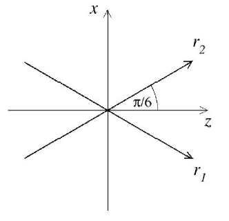
Figure 1: Lines in configuration space along which the electrons are allowed to move. $r_{i}$ denote the position of the electrons along the lines. The angle of $\pi/6$ is chosen such they agree with the motion of the Stark saddle under variation of the field.

A model that keeps the simplicity of the aligned electron models but allows for correlated electron escape was proposed in eckhardt06 . The model builds on the insights gained from classical trajectory studies eckhardt01pra1 . In the presence of the field, each electron sees an effective Stark saddle. Due to electron-electron repulsion the saddles move from the repulsion free positions and are placed symmetrically with respect to the polarization axis and within the same distance from the nucleus. The saddles move along straight lines when the field changes. The observation that the electrons have to cross this saddle then led to the suggestion to restrict the electronic motion to the lines traced by the saddles. The lines form angles of $\pm\pi/6$ with respect to the polarization axis (compare Fig. 1). Since electrons separate as they simultaneously move out from the nucleus their mutual repulsion diminishes, and the resulting potential far from the diagonal, i.e. around $r_{1}=r_{2}$ (where $r_{1}$ and $r_{2}$ are the positions along the saddle lines), becomes quite similar to that of the aligned electron model, as evident from the potential landscapes in Fig. 2. The two potentials differ near the diagonal, where both electrons have the same distance from the nucleus: the diagonal is accessible in the present model, but blocked by Coulomb repulsion in the aligned electron model.

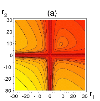
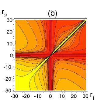
Figure 2: (Color online) Comparison between the potentials (a) for the Hamiltonian (6) used here and (b) the aligned electron model. In the latter case both electrons are restricted to move along the polarization axis, and the diagonal is blocked by the diverging Coulomb repulsion.

As discussed in prauzner07 , this 1D+1D restricted model is able to reproduce the tunnelling and the rescattering processes, as well as a subsequent simultaneous double ionization or other paths to double and single ionization. From the classical mechanics point of view the model has the drawback that the chosen subspace is not an invariant subspace of the full motion, as is the case for the aligned electron model. This drawback is shared with the previously mentioned model of constrained center of mass motion becker . Nevertheless, we will see that the model does yield qualitative predictions and valuable insights into the relevant processes and interactions.

In the new “saddle-track” coordinates the dynamics of two electrons in the linearly polarized laser field is given by the Hamiltonian eckhardt06 :

$$H=\sum_{i=1}^{2}\left(\frac{p_{i}^{2}}{2}-\frac{2}{|r_{i}|}+\frac{F(t)\sqrt{3}}{2}r_{i}\right)+\frac{1}{\sqrt{(r_{1}-r_{2})^{2}+r_{1}r_{2}}},$$ (6)

where $r_{1}$ and $r_{2}$ are the electron coordinates along the saddles’ lines.

III Methods and Procedures

This section is mainly technical and devoted to details of the numerical procedures used in the following sections. The subjects covered in this section include the numerical method in III.1, the partitioning of configuration space in III.2, the calculation of the ionization yields in III.3 and the extraction of the final momentum distributions in III.4. Readers interested mainly in the physical results should read the description in section III.2 of how the different ionization channels are identified in the configuration space, and may then proceed directly to the next section.

III.1 Numerical methods

The simplified 1D+1D model is applied to calculate ionization yields for single and double ionization as well as to obtain electron and ion momenta distributions. The Schrödinger equation corresponding to the Hamiltonian (6) is solved on a grid using the operator splitting method combined with the Fast Fourier Transforms to effectively switch between the position (appropriate for the potential) and the momentum (for the kinetic energy evaluation) representations. The ionization yields are efficiently obtained in the length gauge while the velocity gauge is used for the momenta distributions. In the latter case, the physical space is divided into different regions with Coulomb repulsion neglected in the outer regions (as explained in details below).

The potential singularities in (6) are removed by replacing $1/x$ by $1/\sqrt{x^{2}+e}$ with $e=0.6$. This leads to a ground state energy of the unperturbed atom of $E_{g}=-2.83$ (calculated by means of the imaginary time evolution).

In the time evolution, in order to minimize the undesired reflections at the edges of the integration region, absorbing boundary conditions are included by adding imaginary potentials

$$V_{j}=\left\{\begin{array}[]{c}-i\eta(|r_{j}|-x_{0})^{\alpha},\quad{\rm for}\quad|r_{j}|>x_{0},\\ 0,\quad{\rm elsewhere},\end{array}\right.$$ (7)

where $x_{0}$ is the distance from the center (along each axis) beyond which the imaginary potential becomes active. The value of $x_{0}$ is chosen sufficiently large so as to not perturb the dynamics close to the nucleus, but it is smaller than $L/2$, when the integration domain in one direction is $[-L/2,L/2]$. The parameters $\eta$ and $\alpha$ are optimized with respect to the distance from the edge of the grid, $L/2-x_{0}$, on which absorbing boundary conditions are implemented. We use $\eta=10^{-5}$ and $\alpha=4$ .

III.2 Identifying outgoing channels

Figure 3: Configuration space of the model. The regions labelled A, S_i and D_i correspond to the neutral atom, and singly charged ion, and doubly charged ion populations, respectively. Ionization rates are estimated from the flux across the appropriate borders, and momentum distributions are obtained by propagating the fractions of the wave functions in the corresponding singly and doubly ionized regions (see section III.2 for more details).

For the proper assignment of the final state to the appropriate decay channel we have to identify indicators for single and double ionization. Some guidance as to how to pattern configuration space is provided by the interaction potentials and the regions in which they dominate. As in many other cases, the long range nature of the Coulomb interaction calls for special care, but we will here adopt a pragmatic approach and simply classify state space by the regions in which the interaction is stronger than some threshold. This then results in the division of state space as shown in Fig. 3. We follow in this respect the original ideas developed in the Belfast group taylor . When both electrons are close to the core and interact strongly, the system is in an atomic state, so this region is labelled ${\bf A}$. If one electron escapes along the $r_{1}$-axis and the other is trapped, i.e. $r_{2}$ is bounded, then only the attraction of this second electron to the nucleus remains asymptotically: this defines the bands parallel to $r_{1}$, which are labelled ${\bf S}_{1}$ and ${\bf S}_{3}$ to indicate single ionization (in this case, of electron $1$). Similar considerations lead to the definition of ${\bf S}_{2}$ and ${\bf S}_{4}$ for the single ionization of electron $2$. If both electrons escape, then we have double ionization, indicated by the four regions ${\bf D}_{i}$. The numerical values for the borders between different regions affect the quantitative predictions of the model to some extend. This is not a major problem here since anyway the restricted dimensionality model we consider yields qualitative predictions only. We take the original Belfast proposition taylor for numerical values entering the model (indicated in Fig. 3).

Starting from a state localized near the nucleus, there are several paths to double ionization. A sufficiently strong field will open a Stark saddle along the diagonal, thus enabling the electrons to pass directly from ${\bf A}$ to ${\bf D}_{1}$ and ${\bf D}_{3}$, respectively. We call this simultaneous escape (SE), since both electrons move into the ionized region directly. The processes called REDI for REcollision induced Direct Ionization weber00n are one example of this behaviour. Other contributions could come from situations in which the doubly excited state formed during rescattering persists for a while and does not decay until a later field cycle.

We can also link the different quadrants of our model with the Z and NZ trajectories discussed by Ho et alHo2005 . The Z trajectories have zero or small momenta for the ion, and thus require the electrons to move in opposite directions. A Z trajectory will hence end up in section ${\bf D}_{2}$ or ${\bf D}_{4}$. Such events are allowed, but, according to our calculations, very rare. An NZ trajectory, where the momentum of the ion is non-zero, will end up in sector ${\bf D}_{1}$ or ${\bf D}_{3}$. Note that only the NZ trajectories are influenced by the electron repulsion during their escape, and hence only they will show the momentum correlations in the final state (according to the classical analysis in eckhardt01pra1 )

Other paths to double ionization pass through the single ionization regions ${\bf S}_{i}$ before entering one of the ${\bf D}_{j}$. Such paths are then either purely independent sequential electrons escapes or reminiscent of the RESI processes in longer pulses: Recollision and Excitation of the ion plus Subsequent Ionization RESI . We will collect their signal under the common name: a consecutive escape (CE).

III.3 Ionization yield

With the outgoing channels properly identified, the determination of the physical observables becomes relatively easy. For instance, population of one of the states can be determined by integrating the modulus squared of the wavefunctionover a given region. E.g. the population of atoms follows from

$$P_{A}=\int_{A}|\psi|^{2}{\rm d}r_{1}{\rm d}r_{2}.$$ (8)

However, due to the fact that absorbing boundary conditions are applied, the wavefunctionleaks out of the interaction region, and the norm of the total wavefunctionand the calculated yields decrease with time. To overcome this problem, the yields are instead calculated by using the probability fluxes between appropriate regions, as suggested by Dundas et al. taylor . The fluxes are obtained from the quantum mechanical continuity equation,

$$\frac{\partial}{\partial t}\rho+{\bf\nabla}\cdot{\bf j}=0,$$ (9)

where $\rho=|\psi|^{2}$ is the probability density and ${\bf j}=-i(\psi^{\star}{\bf\nabla}\psi-\psi{\bf\nabla}\psi^{\star})/2$ is the probability current footnote1 . Integration of the continuity equation over a given region ($R\in\{{\rm{\bf A},{\bf S},{\bf D}}\}$) and over time gives the population of the corresponding species:

$$P_{R}(t)=-\int\left(\int_{R}{\bf\nabla}\cdot{\bf j}{\rm d}r_{1}{\rm d}r_{2}\right){\rm d}t=-\int\mathcal{F}_{R}(t){\rm d}t,$$ (10)

where $\mathcal{F}_{R}(t)$ is the probability flux over boundaries of the region $R$.

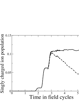
Figure 4: Comparision between the singly charged ion population as calculated using different methods: direct integration of the modulus squared wavefunctionover the regions S_i (dashed line) and integration of the probability fluxes through the boundaries of the S_i regions (solid line). Absorbing boundary conditions were introduced at a distance 150 a.u. from the nucleus and a 5 cycle laser pulse with amplitude $F_{0}=0.19$ a.u. was used.

Fig. 4 compares the population of singly charged ions as a function of time obtained applying both methods described above. The results are for a 5 cycles long laser pulse with amplitude $F_{0}=0.19$. To allow the ionised (possibly slow) electrons to leave the vicinity of the nucleus, here and in all the other calculations the evolution is continued for one additional cycle. The absorbing boundary conditions are set at the distance of $x_{0}=150$ a.u. from the nucleus. As can be seen, as long as the electrons do not reach the absorbing boundaries both methods give the same result. Then, once electrons are absorbed, there is a dramatic fall of the population calculated from the direct integration of the modulus squared wavefunctionover the S_i regions. However, the ionization yield calculated from the probability fluxes remains essentially flat.

To obtain the double ionization yield we calculate fluxes through the boundaries of the D_i regions. This in turn enables us to distinguish between the direct and indirect double ionization events by calculating probability fluxes over relevant boundaries, as discussed before in section III.2. That is, one calculates the flux between regions corresponding to singly and doubly charged ions in order to get the RESI ionization yield, and between regions A and D_i to get the direct double ionization yield.

To summarize:

• The population of single ions (SI) at time $t$ is obtained from time integration of the fluxes from A to S_i ($i=1,2,3,4$) minus the fluxes from S_i to D_j;

• The probabilities for simultaneous double escape (SE) are obtained from the time integration of the fluxes A$\rightarrow$D₁ and A$\rightarrow$D₃.

• A possible simultaneous, anti-correlated double ionization probability is obtained from the time integrals of the fluxes A$\rightarrow$D₂ and A$\rightarrow$D₄.

• Integration of fluxes from S_i to D_j ($i,j=1,2,3,4$) then gives a measure of the consecutive escape (CE), i.e. sequential double ionization and RESI type processes.

III.4 Momentum distributions

At first glance it seems possible to obtain a distribution of electron momenta that corresponds to double ionization by calculating the Fourier transform of the part of the wavefunctionlocalized in the D_i regions (see Fig. 3), using the fact the squared modulus of the wavefunctionin the momentum representation gives a momentum distribution. However, since absorbing boundary conditions are applied, the information contained in the final wavefunctionis not complete: the faster electrons reach quickly the edges of the domain where they are absorbed, and the information about their momenta is lost.

To overcome this problem, we use a method proposed by Lein et al. engel . It is based on the observation that beyond a certain distance from the nucleus, say $x_{C}$ (in the present calculation $x_{C}$ is set to 200 a.u. (except for the results shown in Fig. 15, see text), an electron is unlikely to return. Moreover, since $x_{C}$ is large, the Coulomb potentials are weak and the motion of the electron at that (or an even larger) distance is determined by the field only. Therefore, for distances larger than $x_{C}$, it can be assumed that the electron does not interact with the nucleus and with the other electron. Such a description is reminiscent of the simple man’s model corkum93 that is frequently used to describe the rescattering scenario, but this analogy is only partially correct. In the simple man’s model the interaction with the nucleus and the other electron is neglected directly after the tunnelling event, even when the electron is still close to the nucleus. In our case, Coulomb interactions are neglected only for distances larger than $x_{C}$, where the assumption of a weak interaction is more plausible.

The absence of Coulomb interactions simplifies the subsequent analysis considerably. If one evolves the wavefunctionin the velocity gauge, the interaction with the laser field becomes multiplication by a phase in momentum space. That in turn gives the possibility to efficiently evolve a state in the momentum space as if the configuration space was infinite. Specifically, at the beginning, when both electrons are “close” to the nucleus (this region will be called $R_{in}$), i.e. $|r_{i}|<x_{C}$, the whole evolution is described by the Hamiltonian corresponding to (6) but in the velocity gauge:

$$H_{in}=\sum_{i=1}^{2}\left(\frac{p_{i}^{2}}{2}+\frac{\sqrt{3}}{2}A(t)p_{i}-\frac{2}{|r_{i}|}\right)+\frac{1}{\sqrt{(r_{1}-r_{2})^{2}+r_{1}r_{2}}}.$$ (11)

The wavefunction$\psi(r_{1},r_{2},t)$ spreads during the course of the evolution and eventually some parts of it can enter the outside region $|r_{i}|>x_{C}$, though still remaining well within the extension $[-L/2,L/2]$ of the numerical grid. We want to project out the parts of the wavefunctionin this region and evolve them in a simplified way. This requires some care since the wavefunctionhas to be cut smoothly to minimize reflections on the boundaries. We know that this can be done using absorbing boundary conditions, so we shall use a similar approach with the difference that the “absorbed” part of the wavefunctionwill be further evolved in a simplified way in the outer regions, as we discuss below distance .

To see how the transfer between inner and outer regions is calculated, consider a wavefunction$\psi(r_{1},r_{2})$ that may extend (as indicated by the circle in Fig. 5) beyond the critical distance $x_{C}$. It can be written as a coherent sum of four parts, namely:

$$\psi(r_{1},r_{2}) = \psi_{in}(r_{1},r_{2})+\psi^{1}_{out}(r_{1},r_{2})$$

$$+\psi^{2}_{out}(r_{1},r_{2})+\psi_{out}(r_{1},r_{2}).$$

The $\psi_{in}$ part is the wavefunctionwith both electrons “close” to the nucleus, $|r_{i}|<x_{C}$: the wavefunctionis said to be in the $R_{in}$ region (dashed region in Fig. 5) (with exponential tails in the outside region). This part of the wavefunctionis evolved with the full Hamiltonian (11).

The $\psi^{1}_{out}$ part corresponds to the wavefunctionthat describes a situation where the first electron has crossed the border, but the other one not, i.e. $|r_{1}|>x_{C}$ and $|r_{2}|<x_{C}$ ($R_{1}$ region, shaded area in Fig. 5). Its evolution is governed by Hamiltonian

$$H_{1}=\sum_{i=1}^{2}\left(\frac{p_{i}^{2}}{2}+\frac{\sqrt{3}}{2}A(t)p_{i}\right)-\frac{2}{|r_{2}|}.$$ (13)

which neglects the Coulomb interaction of the outer (first) electron. Thanks to such a simplification, the evolution of the first electron is just a multiplication by a phase factor in the momentum space. The evolution of the other electron still includes the interaction with the nucleus. The $\psi^{2}_{out}$ part has the same meaning, but with regard to the second electron. The last term, $\psi_{out}$, corresponds to the wavefunctionin the region, $R_{out}$ (the white domains in Fig. 5), where Coulomb interactions are neglected. Integration here is done using the Hamiltonian

$$H_{out}=\sum_{i=1}^{2}\left(\frac{p_{i}^{2}}{2}+\frac{\sqrt{3}}{2}A(t)p_{i}\right),$$ (14)

for which it reduces to multiplication by appropriate phase factors in the momentum space.

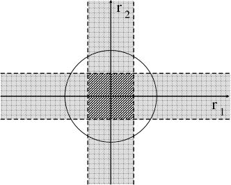
Figure 5: Integration regions for the transfer of the wave functions between the different regions. Dashed lines correspond to borders between the full-integration region (dashed interior region, $R_{in}$), the full-simplified-integration region (white, $R_{out}$), and the semi-simplified-integration regions (shaded, $R_{1}$ and $R_{2}$). The circle indicates the area where the main density of the wavefunctionis located.

In every time step the entire wavefunctionis evolved with the use of the above mentioned Hamiltonians. Then, parts of the wavefunctionthat cross borders are cut and added to the wavefunctionin the appropriate regions.

First, consider the evolved function $\psi_{in}$ It is divided in two parts:

$$\psi_{in}={\tilde{\psi}}_{in}+\Delta\psi_{in}.$$ (15)

The first contribution acquires exponential-like tails outside of the inner region:

$${\tilde{\psi}}_{in}=\left\{\begin{array}[]{ll}\psi_{in},&{\rm for}\quad|r_{i}|<x_{C},\\ D(r_{1})\psi_{in},&{\rm for}\quad|r_{1}|>x_{C},|r_{2}|<x_{C},\\ D(r_{2})\psi_{in},&{\rm for}\quad|r_{1}|<x_{C},|r_{2}|>x_{C},\\ D(r_{1})D(r_{2})\psi_{in},&{\rm for}\quad|r_{i}|>x_{C},\end{array}\right.$$ (20)

where

$$D(r_{i})=\exp\left[-\eta(|r_{i}|-x_{C})^{\alpha}\right].$$ (21)

Here $\eta$ and $\alpha$ are parameters chosen to minimize reflections and take the same values as for the absorbing boundary conditions (see III.1). The part ${\tilde{\psi}}_{in}$ will become the new $\psi_{in}$ function when the process of reorganizing the wavefunctionis completed. The second term is just $\Delta\psi_{in}=\psi_{in}-{\tilde{\psi}}_{in}$ and it is decomposed into three terms:

$$\Delta\psi^{1}_{in} = \left\{\begin{array}[]{ll}\Delta\psi_{in},&{\rm for}\quad|r_{1}|>x_{C},|r_{2}|<x_{C}\\ D(r_{2})\Delta\psi_{in},&{\rm for}\quad|r_{i}|>x_{C},\end{array}\right.$$ (24)

$$\Delta\psi^{2}_{in} = \left\{\begin{array}[]{ll}\Delta\psi_{in},&{\rm for}\quad|r_{1}|<x_{C},|r_{2}|>x_{C}\\ D(r_{1})\Delta\psi_{in},&{\rm for}\quad|r_{i}|>x_{C},\end{array}\right.$$ (27)

$$\Delta\psi_{in}^{out} = \Delta\psi_{in}-\Delta\psi^{1}_{in}-\Delta\psi^{2}_{in}.$$ (28)

These terms will be coherently added to the wave functions in the appropriate regions.

Consider now the $\psi^{1}_{out}$ part evolved under (13) for $|r_{1}|>x_{C}$. The evolved function may extend also into the region where $|r_{2}|$ exceeds $x_{C}$. Thus we define,

$${\tilde{\psi}}^{1}_{out}=\left\{\begin{array}[]{ll}\psi^{1}_{out},&{\rm for}\quad|r_{2}|<x_{C},\\ D(r_{2})\psi^{1}_{out},&{\rm for}\quad|r_{2}|>x_{C},\end{array}\right.$$ (31)

and

$$\Delta\psi^{1}_{out}=\psi^{1}_{out}-{\tilde{\psi}}^{1}_{out}.$$ (32)

The part $\Delta\psi^{1}_{out}$ will be the contribution added to the “double ionization” sector later. The wavefunction$\psi^{2}_{out}$ is treated similarly, with $r_{1}$ and $r_{2}$ interchanged. If the wavefunctionhas a definite parity under exchange, this can efficiently be implemented with the symmetrization eckhardt07 .

Assuming the trivial evolution for $\psi_{out}$ has also been performed we may update the wavefunction. The inner part is just replaced by ${\tilde{\psi}}_{in}$. The part that comes from the inner region is added to the wavefunction in the regions 1 (and 2) and, at the same time, the corresponding part that goes to the outer region is cut from it. The wavefunctionin the outer region has only incoming contributions from all other regions. The update is, therefore, realized by the following sequence:

$$\psi_{in} \rightarrow {\tilde{\psi}}_{in},$$

$$\psi^{1}_{out} \rightarrow {\tilde{\psi}}^{1}_{out}+\Delta\psi^{1}_{in}$$

$$\psi^{2}_{out} \rightarrow {\tilde{\psi}}^{2}_{out}+\Delta\psi^{2}_{in}$$

$$\psi_{out} \rightarrow \psi_{out}+\Delta\psi^{out}_{in}+\Delta\psi^{1}_{out}+\Delta\psi^{2}_{out}.$$ (33)

This sequence is repeated in every time step and of course it is accompanied by appropriate changes of representations from position space to momentum space.

Finally, one can collect all parts of the wave function, add them coherently and obtain the wavefunction of the whole system in the momentum representation.

III.5 Extracting two-electron information

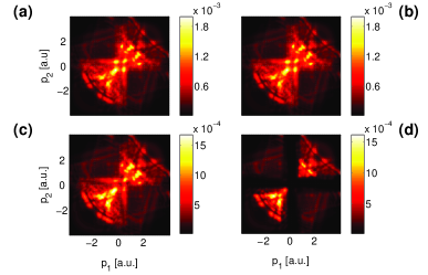
Figure 6: (Color online) Effect of the ionization radius on the electron momentum distribution: (a) $|r_{i}|>$10 a.u., (b) $|r_{i}|>$25 a.u., (c) $|r_{i}|>$50 a.u. and (d) $|r_{i}|>$200 a.u. The calculations are for a laser pulse with an amplitude $F_{0}=0.3$ a.u., a carrier-envelope phase $\phi=0$ and a duration of 5 cycles. The distributions are convoluted with a Gaussian of $\sigma_{p}=0.07$ a.u. width.

We now have access to the whole momentum distribution of our system but we have yet to give the prescription how to extract from the two electron wavefunction the interesting information about the momenta of two ionized electrons. As has been already noted, one can define regions of the coordinate space that are identified with an atom, and singly or doubly charged ions. In order to focus on the double ionization, the parts of the wavefunction corresponding to the atom and to the single ion may be smoothly cut out from the wave function. Those regions form a cross (compare again Fig. 3). Its width may be altered and in such a way the size of the regions corresponding to the atom, the single and the double ionization may be changed. That obviously affects the corresponding momenta distributions.

In Fig. 6 momenta distributions for different cross widths are depicted. The last panel, (d), corresponds to the wave function from the outer region, i.e. $R_{out}$ — $|r_{i}|>200$ a.u. As can be seen, by the cutting out the inner part of the wavefunction identified with the atom or the singly charged ion, one erases small and uncorrelated momenta from the distribution. That momenta are located along axes and close to the center of the coordinate system. Without much loss one could analyze only the part of the wavefunctionthat lies in the $R_{out}$ region – see Fig 6(d) – because it already reveals the key feature of the correlated escape, i.e. a significant population along the diagonal, $p_{1}=p_{2}$. However, comparison with the panel (c) shows that one neglects some of electrons moving in a correlated manner with smaller momenta (note the maxima along the diagonal close to the center of the coordinate system), that do not reach the $R_{out}$ region before the end of integration. Therefore, we have decided that in the following analysis momentum distributions corresponding to the case of $|r_{i}|>50$ a.u. will be considered.

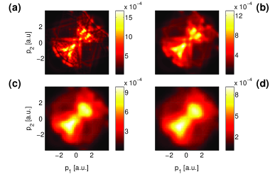
Figure 7: (Color online) Resolution dependence of the final momentum distributions: the distributions are smoothed with Gaussians of width (a) 0.07 a.u., (b) 0.16 a.u., (c) 0.3 a.u., and (d) 0.4 a.u, respectively. The calculations are for a pulse with an amplitude $F_{0}=0.3$ a.u., a carrier-envelope phase $\phi=0$ and 5 cycles duration. Only the wavefunctionin the region $|r_{i}|>50$ a.u. is included in the calculation.

Next we examine the variations of the distributions with resolution. In numerical simulations one could resolve the distributions arbitrarily well, however, at the expense of very long integration times and increasing memory requirements. On the other hand, the experimental distributions are obtained with a finite resolution, only. In order to compare the data obtained with the present model with the experimental ones, we convolute all momenta distributions with Gaussians. To see the effect of this smoothing, momentum distributions obtained with different resolutions, from the presently best experimental resolution of $\sigma_{p}=0.07$ a.u. weckenbrock04 up to a value of $\sigma_{p}=0.4$, are compared in Fig. 7. Panels (c) and (d) resemble experimental distributions weber00n very much, even though only one carrier-envelope phase was used. Panel (d) corresponds to the experimental resolution obtained in the first experiment in which the momenta distributions were measured weber00n . Panels (a) and (b) show considerable substructure, which may have its origin in quantum interferences (see below).

IV Results for smooth pulses

A first batch of results obtained using the above prescription were presented in prauzner07 . There the focus was on flat-top (trapezoidal shaped) pulses that allowed for a clear identification of the relation between the pulse intensity (being constant for the most of the pulse duration) and the ionization dynamics. In another short contribution eckhardt07 we have concentrated on the influence of the symmetry of the wavefunctionon the correlated electron escape. Here, apart from providing some of the technical details, we shall concentrate on smooth laser pulses with electric field amplitude of the form (4). In all the calculations we fix the frequency of the field to be $\omega=0.06$ a.u.

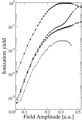
Figure 8: Ionization yields versus field strength. From top to bottom: single ionization (circles), non-simultaneous double ionization (triangles), simultaneous double ionization (squares) and anti-correlated double ionization (crosses). The calculations are for a pulse of five cycles duration.

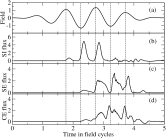
Figure 9: Probability fluxes as a function of time. Panel (a) represents the instantaneous field strengths for a pulse with maximal field amplitude $F_{0}=0.18$ and 5 cycle duration. The flues related to single ionization, to simultaneous ejection and to other consecutive double ionization processes are shown in panels (b), (c) and (d), respectively. All fluxes are in arbitrary units (in particular, recall from Fig. 8 that single ionization fluxes are typically hundreds of times higher than double ionization fluxes).

Consider first the total ionization yields, shown in Fig. 8 for a pulse of five cycles duration and a fixed phase $\phi=0$. The single ionization yield shows the typical behaviour, it reaches almost 100% for high field intensities, and then drops down for still higher fields when the double ionization becomes significant. We observe that:

1. up to a field strength $F_{0}\approx 0.3$, the double ionization yields are several orders of magnitude below the single ionization yield,

2. simultaneous escapes increase strongly until about $F_{0}=0.2$, where the increase becomes noticeably slower,

3. consecutive escapes pick up near about $F_{0}=0.3$, thereby accounting almost exclusively for the knee structure familiar from experimental observations,

4. for five cycle pulses considered here, SE is always less probable than CE where one electron ionizes after the other; the difference is small for low field amplitudes and increases for higher field amplitudes,

5. the signal for anti-correlated electron escape is several orders of magnitude smaller than that for other processes. Its non-zero value may actually have a numerical origin, and be connected with the calculation of the flux at a finite distance from the nucleus.

The consecutive ionisation process may consist of at least two paths: the independent electron escape where, after the escape of the first electron, the other has to get rid of the nucleus’ attraction on its own (this process becomes more significant for $F_{0}$ above the knee) and the process where due to the rescattering the second electron is first excited and then, after the first electron is already gone, it leaves the ion too. The rescattering may be repeated several times, thus contributing to an increase of both the simultaneous and consecutive escapes.

More information about the dynamics of the ionization process, in particular about the temporal sequence of events and the timing of double ionization during the pulse, may be extracted by following the time dependencies of the probability fluxes. They are shown in Fig. 9, together with the field amplitude. Note the strong correlation between panels (b) and (c) with pronounced maxima for the SE flux occurring about half a cycle after the SI flux maxima: this is a direct confirmation of the rescattering scenario. First, the electron leaves the A region, evidenced in Fig. 9b by the peaks in the single ionization flux near the field extrema, when the saddle for the single ionization is open and the ionization itself is the most probable. Then the electron is turned back to the nucleus and gains energy as it is accelerated by the field. It hits its parent ion and shares its energy with the electron near the core to form a highly excited state. This highly excited compound state then decays through single, simultaneous escape and consecutive double ionization. This is seen as peaks in fluxes into both channels that appear roughly one half-cycle later than the corresponding peaks in the single ionization flux (see Fig. 9). In the first half of the pulse single ionization dominates; then, once there is enough time for the electron to turn back and to rescatter, double ionization follows, see Fig. 9c and d. Moreover, both types of double ionization events occur close to the laser field extrema. In the case of simultaneous double escape, this means that the field is sufficiently large to open the saddle for the symmetric escape. This observation is at variance with expectations based on the simple man model corkum93 , but in agreement with previous deductions from the analysis of the classical paths eckhardt01pra1 ; eckhardt06 .

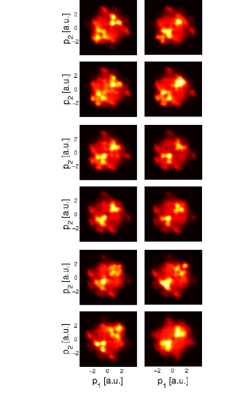
Figure 10: (Color online) Phase dependence of the electron momentum distributions. The phases increase from left to right and top to bottom from $\phi=0$, $0.1\pi$, $...$, to $\pi$. Note that the frame on the bottom left for $\phi=\pi$ is the mirror image of the one on the top left for $\phi=0$, reflecting the mirror symmetry in the pulses. The frame on the bottom right is obtained for a uniform average over all phases. The calculations are for a pulse with $F_{0}=0.2$ and a five cycle duration. The distributions are convoluted with a Gaussian of $\sigma_{p}=0.2$ a.u. width, and only the wave functions in the region $|r_{i}|>50$ a.u. is shown.

The electron momenta distributions for different carrier-envelope phases are shown in Fig. 10. The chosen value of the field amplitude $F_{0}$ corresponds to the beginning of the knee structure in Fig. 8. Observe that, regardless of the phase, a significant fraction of the electrons are ejected with similar momenta $p_{1}\approx p_{2}$, as the distributions are diagonally dominated.

The momentum distributions show a significant dependence on the carrier envelope phase of the pulse. Apart from the obvious global symmetry corresponding to the change of $\phi$ by $\pi$, which is equivalent to the change of the sign of the momenta, one observes rapid changes of distributions corresponding to small changes of phases (compare e.g. panels corresponding to $\phi=0.1\pi$ and $\phi=0.2\pi$, or $\phi=0.5\pi$ and $\phi=0.6\pi$). This behaviour conforms with classical and analytical studies liu04 ; maciek2004 , that even propose to use the momentum distributions for the identification of the laser pulse phase. We will return to the differences in fine-structure in the next section.

In addition to the electron momentum distributions, we can also study the ion momentum distribution, see Fig. 11. Within the model, the ion distribution is nothing but the negative of the sum of electron momenta, corrected by the geometrical factor due to the $\pi/3$ angle between the axes, (see Fig. 1), i.e. $p_{\rm ion}=-\sqrt{3}(p_{1}+p_{2})/2$. When averaged over a uniform distribution of phases under a carrier envelope this distribution is symmetric and shows the celebrated double-hump structure.

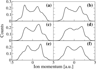
Figure 11: Phase difference of the ion momentum distribution. The phases are (a) $\phi=0$, (b) $3\pi/10$, (c) $\pi/2$, (d) $4\pi/5$, and (e) $\pi$. Note that the distributions for $\phi=0$ and $\phi=\pi$ in (a) and (e) differ by a reflection of the ion momentum, only. Panel (f) shows the distribution averaged over a uniform $\phi$ distribution. The calculations are for a pulse with $F_{0}=0.2$ and five cycle duration.

V Interference fringes in momenta distributions

In almost all momenta distributions presented until now one could notice substructures that are reminiscent of quantum interference patterns. Within a semi classical picture, the coherence of the wavefunctionis maintained, and the pattern could arise from interferences between contributions from several paths to the same final momenta. Some of these paths have been seen within classical trajectory studies eckhardt06 . Arbó et al. burgdoerfer have also shown that ionization events originating at different times during a pulse can contribute to the ionization signal and give rise to interferences. In all cases the substructures require a good resolution in order to be resolved (recall the effects of resolution shown in Fig. 7). Therefore, in this section, we shall work with a resolution of $0.07$ a.u., as is accessible in the best current experiments weckenbrock04 .

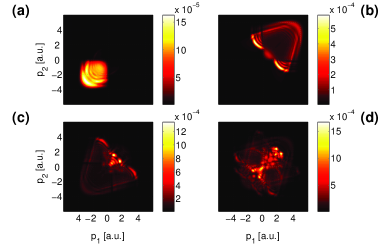
Figure 12: (Color online) Effect of pulse length on momentum distributions. The length of the pulse is (a) one cycle, (b) two cycles, (c) three cycles, (d) four cycles. The calculations are for a pulse with an amplitude $F_{0}=0.3$ a.u., and a carrier-envelope phase $\phi=0$. The wavefunctioncorresponding to the region $|r_{i}|>50$ a.u. is shown. The distributions are convoluted with a Gaussian of width $\sigma_{p}=0.07$ a.u.

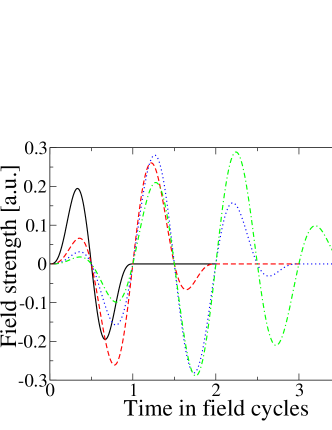
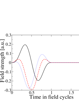
Figure 13: (Color online) Variations in instantaneous field strength with duration and phase of the pulse. The pulses have a field amplitude $F_{0}=0.3$ a.u.. For the top panel, the carrier-envelope phase is set to $0$ , and the duration is one cycle (black solid line), two cycles (red broken line), three cycles (blue dotted line) and four cycles (green dash-dotted line). For the bottom panel, the duration of the pulse is fixed to be a single cycle, and the phases are $0$ (black solid line), $0.5\pi$ (red broken line) and $0.7\pi$ (blue dotted line).

The observed pattern depends on several parameters of the problem, including the amplitude of the field, the pulse duration and the carrier-envelope phase. Among them, the pulse duration seems to be the most critical for a theoretical understanding of the process, in that the shorter the pulse, the smaller the number of possible paths that lead to double ionization. The increase in complexity is demonstrated in Fig. 12, where momenta distributions for pulses of different duration are shown. Apparently, each additional cycle increases the complexity of the pattern.

However, the pulse duration is not the only reason for the observed differences. Because of the ramping of the field, the actual maximal instantaneous field strength that is reached during the pulse may be lower than the nominal amplitude $F_{0}$, and may vary with the envelope function and the phase of the field, see Fig. 13, where the actual field amplitudes for the momentum distributions of Fig. 12 are shown. The black solid line in the top panel corresponds to the single cycle pulse and the maximal instantaneous effective field amplitude is $F_{max}=0.19$ a.u., even though the nominal pulse amplitude is set to be $F_{0}=0.3$ a.u. For the longer pulses the maximal field amplitude becomes $F_{max}=0.25$, $0.28$, and $0.29$ a.u. for pulses with two, three and four cycles, respectively. The maximal field strength agrees with $F_{0}$ for longer pulses.

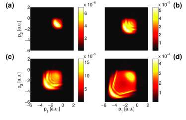
Figure 14: (Color online) Electron momentum distributions corresponding to the single cycle laser pulse for $\phi=0$ and $F_{0}=0.2$, $0.25$, $0.3$, and $0.4$ [from (a) to (d)]. Note that the interference fringes appear for larger field amplitude only. The wavefunctioncorresponding to the region $|r_{i}|>50$ a.u. is shown. The distributions are convoluted with a Gaussian of $\sigma_{p}=0.07$ a.u. width.

To simplify the picture we shall consider in the following the single cycle pulse only. Fig. 14 shows the momentum distributions for a sine-squared envelope and different field amplitudes $F_{0}$. For higher field amplitudes $F_{0}$, the momentum distribution reveals interesting interference patterns. While the detailed analysis of their origin requires extensive semiclassical studies that are beyond the scope of the present paper, we attempt below a qualitative understanding of the phenomenon.

Let us now consider how the absolute phase of the laser pulse affects the interference pattern. This dependence can be expected to be quite dramatic, in view of earlier observations for few cycle pulses (compare Fig. 10). Note also the strong dependence of the effective electric field temporal behaviour on the phase, Fig. 13. It turns out that the interference fringes are present for the carrier-envelope phase close to $\phi=0$ only. Then the absolute value of the field has two maxima of comparable amplitude. For other values of the phase a single maximum (of the absolute value) dominates the field temporal behaviour.

That in turn points out strongly towards a rescattering scenario as a necessary ingredient of the appearance of the fringes. The first field maximum excites a single electron, it turns back after the field direction changes and as a highly energetic particle shares its energy with the remaining electron leading to a double ionization. Such a process is less probable for a singly peaked field.

In order to study further the significance of the rescattering for the presence of the fringes, we repeated the time evolution with different (smaller) $x_{C}$ which determines the ionization regions, thereby limiting the electronic motion (leading to rescattering) to area close to nucleus (once an electron reaches the distance $x_{C}$ from the nucleus its evolution is simplified by neglecting Coulomb potentials, see Sec. IIID). Such an approach has been used recently to discuss the influence of long rescattering orbits in non sequential double ionization of the hydrogen molecule baier06 . We focus on momentum distributions for two phases; those for $\phi=0$ that show interference patterns, and the other for $\phi=0.5\pi$ that do not show them in Fig. 15. The gradual disappearance of the fringes in the left column when $x_{C}$ decreases suggests that the existence of the interference pattern is linked to the rescattering process.

The situation is not that simple, however. Additional classical trajectory studies indicate that even for small $x_{C}=12.5$ a.u. values there exist rescattering trajectories; those, however, extend less from the nucleus. The fringes are thus most probably due to the quantum interference of contributions coming from “long” and “short” rescattering orbits. The latter only are eliminated by restricting the interaction between the electrons to the area very close to the nucleus.

The interference phenomena due to “long” and “short” trajectories has been discussed in the context of high-harmonic generation several years ago lewenstein94 ; becker94 . It seems that the very same trajectories are responsible for the interference pattern in the momenta distribution of the outgoing electrons in double ionization process.

The absence of any changes in the right column suggests that for this phase of the field the contribution of long rescattering orbits is smaller, hence supporting a more direct double ionization process. Note that in the latter case, i.e. $\phi=0.5\pi$, the field possesses very strong maximum in the middle of the pulse (see Fig. 13b) that weakens the rescattering effect.

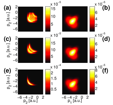
Figure 15: (Color online) Effect of rescattering on momentum distributions. (a) and (b) show the momentum distributions for $\phi=0$ and $\phi=0.5\pi$, respectively, as obtained with the cut-off $x_{C}=50$ a.u.. For (c) and (d), the cut-off is reduced to $x_{C}=25$ a.u., and for (e) and (f) to $x_{C}=12.5$ a.u.. Decreasing the cut-off reduces the contributions from rescattered electrons, and the contrast in the interference pattern. The calculations are for a laser pulse with an amplitude $F_{0}=0.3$ a.u. and a pulse duration of one cycle. The momentum distributions are calculated from wave functions in the regions $|r_{i}|>50$ a.u. and are convoluted with a Gaussian of width $\sigma_{p}=0.07$ a.u.

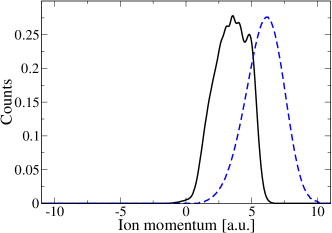
Figure 16: (Color online) Ion recoil momenta distributions corresponding to electron momenta distributions of Fig. 15. Black solid line corresponds to $\phi=0$ and reveals a ragged top with several maxima, reflecting the interferences shown in left panels of Fig. 15. The dashed line represents the distribution for $\phi=0.5\pi$; it is smooth, in accord with the absence of interferences in the right column of Fig. 15

As discussed before, the electron momentum distributions yield in a direct way the ion recoil momentum distributions. The latter, for the field strengths and phases of Fig. 15, are presented in Fig. 16. The presence of interferences in the electron momenta shows up in the ion momentum distribution in the form of a ragged maximum. Since ion recoil momentum distributions can be measured experimentally, the transition between ragged and smooth maxima should be readily accessible to experimental verification.

VI Conclusions

The calculation of wave functions and ionization events and their interpretation presented here show that the reduced dimensionality model proposed in eckhardt06 captures many of the features of the quantum double ionization process. The knee structure in the ionization yield, the double hump structure in the ion momentum distribution and the electron momentum distributions are in agreement with observations, and the results on the phase dependence and the interference patterns suggest further experimental and theoretical studies. The major advantage of the present model over the well known and much studied aligned electron model is that it does allow for the correlated two-electron escape which is blocked in the aligned model by the overestimated Coulomb repulsion.

We have discussed the details of the numerical implementation of the model as well as the methods that enable us to extract the relevant physical information from the dynamically evolved wavefunction. We have discussed the ionization features for smooth few cycle pulses as well as for very short pulses (up to a single cycle pulses). For the former we have confirmed that the model yields prediction in a qualitative agreement with experimental data for all the calculated observables (ion yield, ion recoil and electron momenta distributions). We have confirmed previous suggestions liu04 ; maciek2004 that the absolute phase of the pulse carrier envelope may be extracted from the momenta distributions. For even shorter pulses the phase dependence of the signals becomes quite dramatic. The electron momentum distributions show distinct interference patterns which are traces of different paths leading to double ionization. With a sufficient resolution these interference patterns can also be seen in longer pulses, however their complexity grows significantly with the pulse duration. The fringes provide additional information about the absolute phase but also are manifestations of nontrivial dynamics. Interestingly, their very existence seems to be intimately connected to the rescattering process. The interferences can also be seen in ion recoil momentum distributions, and hence should be quite easily accessible in experiments that do not resolve the electron momentum distributions.

VII Acknowledgements

A significant part of the numerical simulations were done at ICM UW under grant G29-10. The work has been supported by the Deutsche Forschungsgemeinschaft and Marie Curie ToK project COCOS (MTKD-CT-2004-517186). Support by the Polish Government scientific funds (2005-2008) as a research project is acknowledged.

References

- (1) S. Geltman and J. Zakrzewski, J. Phys. B 21, 47 (1988).
- (2) A. L’Huillier, L. A. Lompre, G. Mainfray, and C. Manus, Phys. Rev. Lett. 48, 1814 (1982).
- (3) A. Becker, R. Dörner, and R. Moshammer, J. Phys. B 38, S753 (2005).
- (4) B. Walker et al., Phys. Rev. Lett. 73, 1227 (1994)
- (5) T. Weber et al., Nature 405, 658 (2000); T. Weber et al., Phys. Rev. Lett. 84, 443 (2000); R. Moshammer et al., Phys. Rev. Lett. 84, 447 (2000).
- (6) A. Becker and F. H. M. Faisal, Phys. Rev. Lett. 84, 3546 (2000); R. Kopold et al., Phys. Rev. Lett. 85, 3781 (2000).
- (7) R. Grobe and J. H. Eberly, Phys. Rev. Lett. 68, 2905 (1992); R. Grobe and J. H. Eberly, Phys. Rev. A 48, 4664 (1993); D. Bauer, Phys. Rev. A 56, 3028 (1997); D. G. Lappas and R. van Leeuwen, J. Phys. B 31, L249 (1998); W.-C. Liu, J. H. Eberly, S. L. Hann, and R. Grobe, Phys. Rev. Lett. 83, 521 (1999); S. L. Haan et al., Phys. Rev. A 66, 061402(R) (2002).
- (8) M. Lein, E. K. U. Gross, and V. Engel, Phys. Rev. Lett. 85, 4707 (2000).
- (9) C. Ruiz et al., Phys. Rev. Lett. 96, 053001 (2006).
- (10) D. Dundas, K. T. Taylor, J. S. Parker, and E. S. Smyth, J. Phys. B 32, L231 (1999);
- (11) J. Parker et al., Phys. Rev. Lett. 96, 133001 (2006).
- (12) P. B. Corkum, Phys. Rev. Lett. 71, 1994 (1993); K. Kulander, J. Cooper, and K. Schafer, Phys. Rev. A 51, 561 (1995).
- (13) K. Sacha and B. Eckhardt, Phys. Rev. A 63, 043414 (2001); B. Eckhardt and K. Sacha, Europhys. Lett. 56, 651 (2001).
- (14) B. Eckhardt and K. Sacha, J. Phys. B: At. Mol. Phys. 39, 3865 (2006).
- (15) J. S. Prauzner-Bechcicki, K. Sacha, B. Eckhardt, and J. Zakrzewski, Phys. Rev. Lett. 98, 203002 (2007).
- (16) R. V. Jensen, Phys. Rev. A30, 386 (1984).
- (17) J.G. Leopold and D. Richards, J. Phys B22, 1931 (1989); ibid. 24, 1209 (1991).
- (18) Q. Su, J. H. Eberly, and J. Javanainen, Phys. Rev. Lett 64, 862 (1990); V. C. Reed, P. L. Knight, and K. Burnett, Phys. Rev. Lett 67, 1415 (1991).
- (19) P.J. Ho and J.H. Eberly, Optics Express 11, 2826 (2003); P.J. Ho, R. Panfili, S. L. Haan, and J.H. Eberly, Phys. Rev. Lett., 94, 093002 (2005); P.J. Ho and J.H. Eberly, Phys. Rev. Lett., 95, 193002 (2005).
- (20) B. Feuerstein et al., Phys. Rev. Lett. 87, 043003 (2001); V.L.B. de Jesus et al., J. Phys. B. 37, L161 (2004).
- (21) It is worth stressing that the probability current has this form only in the position gauge. In the velocity gauge it would also depend on the vector potential, .
- (22) In fact the distance , at which we neglect the Coulomb interactions, and , at which the boundary conditions start to act, are taken to be the same in the numerical implementation.
- (23) B. Eckhardt, J. S. Prauzner-Bechcicki, K. Sacha, and J. Zakrzewski, Phys. Rev. A 77, 015402 (2008).
- (24) X. Liu and C. Figueira de Morrison Faria, Phys. Rev. Lett. 92, 133006 (2004).
- (25) C. Figueira de Morrison Faria, X. Liu, A. Sanpera, and M. Lewenstein, Phys. Rev. A 70, 043406 (2004).
- (26) D.G. Arbó, S. Yoshida, E. Persson, K. I. Dimitriou, and J. Burgdörfer, Phys. Rev. Lett. 96, 143003 (2006); D.G. Arbó, E. Persson, and J. Burgdörfer, Phys. Rev. A 74, 063407 (2006).
- (27) S. Baier, C. Ruiz, L. Plaja, and A. Becker, Phys. Rev. A 74, 033405 (2006).
- (28) M. Lewenstein et al., Phys. Rev. A 49, 2117 (1994).
- (29) W. Becker, S. Long, and J.K. McIver, Phys. Rev. A 50, 1540 (1994).
- (30) M. Weckenbrock et al., Phys. Rev. Lett. 91, 123004 (2003); M. Weckenbrock et al., Phys. Rev. Lett. 92, 213002 (2004).