Compressed low Mach number flows in astrophysics: a nonlinear Newtonian numerical solver

Abstract

Context. Internal flows inside gravitationally stable astrophysical objects, such as the Sun, stars and compact stars are compressed and extremely subsonic. Such low Mach number flows are usually encountered when studying for example dynamo action in stars, planets, the hydro-thermodynamics of X-ray bursts on neutron stars and dwarf novae. Treating such flows is numerically complicated and challenging task

Aims. We aim to present a robust numerical tool that enables modeling the time-evolution or quasi-stationary of stratified low Mach number flows under astrophysical conditions.

Methods. It is argued that astrophysical low Mach number flows cannot be considered as an asymptotic limit of incompressible flows, but rather as highly compressed flows with extremely stiff pressure terms. Unlike the pseudo-pressure in incompressible fluids, a Possion-like treatment for the pressure would smooth unnecessarily the physically induced acoustic perturbations, thereby violating the conservation character of the compressible equations.
Moreover, classical dimensional splitting techniques, such as ADI or Line-Gauss-Seidel methods are found to be unsuited for modeling compressible flows with low Mach numbers.

Results. In this paper we present a nonlinear Newton-type solver that is based on the defect-correction iteration procedure and in which the Approximate Factorization Method (AFM) is used as a preconditioner. This solver is found to be sufficiently robust and is capable of capturing stationary solutions for viscous rotating flows with Mach number as small as $\mathcal{M}\leavevmode\nobreak\ \approx\leavevmode\nobreak\ 10^{-3},$ i.e., near the incompressibility limit.

Received … / Accepted …

1 Introduction

Among different energy contents, the gravitational and thermal energies in bound astrophysical systems are dominant. The virial theorem states that in the absence of external pressure and surface tension the total energy of gravitationally bound system is negative, i.e.,

$$-\alpha_{1}\frac{GM^{2}}{R}+2\left[\mathcal{E}_{\mathrm{th}}+\mathcal{E}_{\mathrm{kin}}\right]+\beta_{1}\frac{\Phi^{2}}{R}<0,$$ (1)

where $\alpha_{1},\beta_{1}$ are constants less than one and where

$$\left\{\begin{array}[]{ll}{Gravitational\leavevmode\nobreak\ energy}:&\mathcal{E}_{\mathrm{grav}}=\mathrm{\frac{GM^{2}}{R}}\\ Thermal\leavevmode\nobreak\ energy:&\mathcal{E}_{\mathrm{th}}=\mathrm{\frac{3}{2}\int_{V}P\leavevmode\nobreak\ dvol}\\ Kinetic\leavevmode\nobreak\ energy:&\mathcal{E}_{\mathrm{kin}}=\mathrm{\frac{1}{2}\int_{V}\rho|V_{f}|^{2}\leavevmode\nobreak\ dvol}\\ Magnetic\leavevmode\nobreak\ energy:&\mathcal{E}_{\mathrm{mag}}=\mathrm{\frac{{\Phi}^{2}}{R}},\end{array}\right.$$ (2)

where $\mathrm{G,\leavevmode\nobreak\ \Phi,\leavevmode\nobreak\ M,\leavevmode\nobreak\ R,\leavevmode\nobreak\ P,\leavevmode\nobreak\ V_{f}},$ denote respectively the gravitational constant, the magnetic flux, the mass and radius of the object, pressure and fluid-velocity, and $\leavevmode\nobreak\ dvol$ is an infinitesimal volume-element.

The final stage in the evolution of such gravitationally stable systems is characterized by the following energy measure:

$$|\mathcal{E}_{\mathrm{grav}}|\geq|\mathcal{E}_{\mathrm{th}}|\gg|\mathcal{E}_{\mathrm{kin}}|,|\mathcal{E}_{\mathrm{mag}}|.$$ (3)

In terms of velocities per mass this relation is equivalent to:

$$\rm{V^{2}_{g}\geq V^{2}_{S}>>V^{2}_{f},V^{2}_{A}},$$ (4)

where the velocities correspond to the self-gravitating energy $(\rm{V^{2}_{g}}\doteq\frac{GM^{2}}{R})$, thermal, fluid and magnetic ($\rm Alfv\acute{e}n$) velocities.

Therefore, fluid motions in gravitationally stable astrophysical systems are naturally sub-sonic, hence the Mach number is relatively low.

For example, helioseismology measurements have revealed that the Sun oscillates on various frequencies. In particular, it has been found that the origin of the 5-minute oscillations is a self-excited sound wave travelling back-and forthwards through the Sun interior (Musman, 1974). This corresponds roughly to the sound speed:

$$V_{\mathrm{S}}\sim\frac{R_{\odot}}{\mathrm{5\leavevmode\nobreak\ minutes}}\approx\leavevmode\nobreak\ 2.3\times 10^{8}\leavevmode\nobreak\ \mathrm{cm\leavevmode\nobreak\ s^{-1}}.$$ (5)

Roth et al. (2002) have suggested that internal flows can have a maximum sectorial amplitude of about $10^{3}\leavevmode\nobreak\ \mathrm{cm\leavevmode\nobreak\ s^{-1}}$. They argue that a higher velocity would lead to a noticable distortion of the rotation rate in the convection zone, hence contradicts observations. In this case, the Mach number reads:

$${\mathcal{M}}=\frac{V_{\mathrm{HD}}}{V_{\mathrm{S}}}\sim 10^{-4}.$$ (6)

Consequently, the fluid motions in the Sun is compressible with extremely low Mach numbers.

Similarly, in the case of neutron stars, the temperature of the superfluid ranges between $10^{7}$ up to $5\times 10^{8}$ K, depending on the crust heat source (Van Riper, 1991). The superfluid velocity relative to coordinates rotating with angular velocity $\Omega_{\mathrm{NS}}$ can reach ${\rm{V_{\mathrm{HD}}}\approx 10^{4}-10^{6}\leavevmode\nobreak\ \leavevmode\nobreak\ cm\leavevmode\nobreak\ s^{-1}}$ (Jones, 2003).
Thus, the ratio of the sound crossing time to the hydrodynamical time scale reads:

$$\frac{\tau_{\mathrm{S}}}{\tau_{\mathrm{HD}}}\approx\left(\frac{V_{\mathrm{HD}}}{V_{\mathrm{S}}}\right)^{2}={\mathcal{M}}^{2}\approx 10^{-6},$$ (7)

where $V^{2}_{\mathrm{S}}[=dP/d\rho=(\rho-\frac{1}{3}p)/(\rho+p)]$ corresponds to the the sound speed squared, which is roughly $10\%$ the speed of light, depending on the equation of state.

The flows in these two extreme astrophysical objects indicate that numerical solvers should be robust enough to deal with extremely low Mach number flows. Such flow-conditions are encountered when trying to model the origin of the solar dynamo or the thermonuclear ignition of hydrogen rich matter on the surface of neutron stars, considered to be responsible for Type-I X-ray bursts (Fisker et al., 2005) or for novae eruption in the case of white dwarfs (Camenzind, 2007).

2 Compressible versus weakly and strongly incompressible flows

While the equations describing compressible and incompressible flows are apparently similar, the underlying physics and the corresponding numerical treatments are fundamentally different.

In general, compressible flows are made of plasmas. The internal macroscopic motions may become either supersonic or extremely subsonic. Incompressible flows however, are generally made of liquid, so that a further compression would not lead to a noticeable change of their density. The transition from gas phase into fluid phase mostly does not occur via smooth change of the equation of state. For example, a high pressure acting onto a container of hot water vapor cannot be asymptotically extended to describe the pressure in normal water fluid. Therefore, from the astrophysical point of view, weakly incompressible flows can be viewed as strongly compressed plasmas, in which the macroscopic velocities are relatively small compared to the sound velocity.

To clarify these differences, we write the set of hydrodynamical equations in non-dimensional form using the scaling variables listed in Table (1).

Scaling	variables	neutron star(interior)
$\tilde{L}$	Length	$\sim\leavevmode\nobreak\ 10^{6}\leavevmode\nobreak\ \mathrm{cm}$
$\tilde{\rho}$	Density	$\sim\leavevmode\nobreak\ 10^{14}\rm{\leavevmode\nobreak\ g\leavevmode\nobreak\ cm^{-3}}$
$\tilde{\mathcal{T}}$	Temperature	$\sim\leavevmode\nobreak\ 10^{7}$ K
$\tilde{\mathcal{P}}$	Pressure	$\sim\leavevmode\nobreak\ 10^{26}\leavevmode\nobreak\ \mathrm{dyn\leavevmode\nobreak\ cm^{-2}}$
$\tilde{V}$	Velocity	$\sim\leavevmode\nobreak\ 10^{6}\leavevmode\nobreak\ \rm{cm\leavevmode\nobreak\ s}^{-1}$
$\tilde{B}$	Magnetic Fields	$\sim\leavevmode\nobreak\ 10^{9}\leavevmode\nobreak\ G$
$\tilde{\mathcal{M}}$	Mass	$\sim\leavevmode\nobreak\ M_{\odot}$

Table 1: Scaling variables for non-dimensioning the hydrodynamical equations.

The set of hydrodynamical equations describing compressible plasmas in conservative form reads:

• Continuity equation:

  $$\frac{\partial\rho}{\partial t}+\nabla\cdot\rho V=0,$$ (8)

• The momentum equations:

  $$\frac{\partial\rho V}{\partial t}+\nabla\cdot(\rho V\otimes V)=-\frac{1}{\mathcal{M}^{2}}\nabla P+\frac{\rho}{\mathrm{Fr}^{2}}\nabla\Psi+\left(\frac{\mathcal{M}_{\mathrm{mag}}}{\mathcal{M}}\right)^{2}{\nabla\times B\times B}+\frac{1}{\mathrm{Re}}\nabla\cdot\sigma,$$ (9)

  where $\sigma(=\eta(\nabla V+(\nabla V)^{\mathrm{T}})-\frac{2}{3}\eta(\nabla\cdot V)I),\leavevmode\nobreak\ \eta=\rho\nu\leavevmode\nobreak\ \mathrm{\leavevmode\nobreak\ and\leavevmode\nobreak\ },$ $\nabla\Psi$ are the Reynolds stress tensor, the dynamical viscosity coefficient and the gradient of the potential energy, respectively.

• The total energy equation:

  $$\frac{\partial\mathcal{E}}{\partial t}+\nabla\cdot(\mathcal{E}+p)V=\mathrm{(\frac{\mathcal{M}}{Fr})^{2}}\leavevmode\nobreak\ \rho\nabla\Psi\cdot V+\mathrm{(\frac{\mathcal{M}}{Re})^{2}}\leavevmode\nobreak\ \nabla\cdot(V\sigma)+\mathrm{\frac{1}{Pe}}\leavevmode\nobreak\ \nabla\cdot(\nu_{\mathrm{T}}\nabla T),$$ (10)

  where $\mathcal{E}=\rho(\varepsilon+\frac{1}{2}\mathrm{V}^{2})\leavevmode\nobreak\$ and $\nu_{\mathrm{T}}$ is the heat diffusion coefficient.
  We may simplify the total energy equation by separating the internal energy from the mechanical energy and assuming a perfect conservation of the latter. Hence, we are left with an equation that describes the time-evolution of the internal energy:

  $$\frac{\partial\mathcal{E}^{\mathrm{d}}}{\partial t}+\nabla\cdot\mathcal{E}^{\mathrm{d}}V=-(\gamma-1)\mathcal{E}^{\mathrm{d}}\nabla\cdot V+(\gamma-1)\{\left(\frac{\mathcal{M}}{\mathrm{Re}}\right)^{2}\Upsilon+\frac{1}{\mathrm{Pe}}\nabla\cdot(\nu_{\mathrm{T}}\nabla T)\},$$ (11)

  where $\Upsilon(\doteq\eta|\nabla\cdot V|^{2})$ is the dissipation function.

• Magnetic equation
  The magnetic induction equation, taking into account transport and diffusion in non-dimensional form reads:

  $$\frac{\partial B}{\partial t}=\nabla\times\langle V\times B-\mathrm{\frac{1}{Re^{\mathrm{mag}}}\leavevmode\nobreak\ (\frac{\mathcal{M}^{\mathrm{mag}}}{\mathcal{M}})}\leavevmode\nobreak\ \leavevmode\nobreak\ \nabla\times B\rangle.$$ (12)

Name	Symbol	Definition
Reynolds number	Re	$\mathrm{{\tilde{V}\leavevmode\nobreak\ \tilde{L}}/{\nu}}$
Mach number	$\mathcal{M}$	$\mathrm{\tilde{V}/\tilde{V}_{\mathrm{S}}}$
Reynolds number (magnetic)	$\mathrm{Re^{\mathrm{mag}}}$	$\mathrm{\tilde{V}\leavevmode\nobreak\ \tilde{L}}/{\nu^{\mathrm{mag}}}$
Mach number (magnetic)	$\mathcal{M}^{\mathrm{mag}}$	$\mathrm{\tilde{V}_{\mathrm{A}}/\tilde{V}_{\mathrm{S}}}$
Prantl number	Pr	$\mathrm{\nu/\nu_{\mathrm{T}}}$
Froude number	Fr	$(\mathrm{\tilde{V}/\tilde{V}_{g}})^{2}$
Peclet number	Pe	$\mathrm{Re\cdot Pr}$

Table 2: Nondimensional numbers. In this list, the additional parameters $\nu,\leavevmode\nobreak\ \nu^{\mathrm{mag}},\leavevmode\nobreak\ \nu_{\mathrm{T}}$ and $\tilde{V_{g}}$ correspond to hydrodynamical viscosity coefficient, magnetic diffusivity coefficient, heat diffusion coefficient and to the effective velocity of the potential energy $\Psi$(i.e., $\tilde{V}^{2}_{g}=\nabla\tilde{\Psi},$ respectively.

On the other hand, incompressible flows are described through the following set of equations:

$$\nabla\cdot V=0.$$ (13)

$${\mathcal{M}^{2}}\,\rho\left[V_{t}+(V\cdot\nabla)V\right]=-\nabla P+\frac{\mathcal{M}^{2}}{\rm{Fr^{2}}}\rho\,\nabla\Psi+\frac{{\mathcal{M}^{2}}}{\mathrm{Re}}\nabla\cdot\sigma$$ (14)

$$\frac{\partial T}{\partial t}+\nabla\cdot TV=(\gamma-1)\{\left(\frac{\mathcal{M}}{\mathrm{Re}}\right)^{2}\leavevmode\nobreak\ \Upsilon+\frac{1}{\mathrm{Pe}}\nabla\cdot({\nu_{\mathrm{T}}}\nabla T)\},$$ (15)

Despite the apparent similarity, the pressure in compressible flows has different physical meaning; in the compressible case the equation of energy influences the momentum equation through the equation of state, whereas in the incompressible case, the pressure is just a lagrangian multiplier with no direct physical meaning. The set of equations of incompressible flows is characterized by the following two features:

1. The velocity field must not only evolve as described by the momentum equations, it should fulfill the divergence-free condition also.

2. there is no direct equation that describes the time-evolution of the pressure.

Therefore, we may use the pressure in the momentum equations to form an equation that enforces the flow to move in such a manner that the divergence-free condition is always fulfilled, independent of the constitutive nature of the flow.

This can be achieved by taking the divergence of the momentum equation above:

$$\nabla\cdot\left[{\mathcal{M}^{2}}\,\rho\left[V_{t}+(V\cdot\nabla)V\right]-\frac{\mathcal{M}^{2}}{\rm{Fr^{2}}}\rho\,\nabla\Psi-\frac{{\mathcal{M}^{2}}}{\mathrm{Re}}\nabla\cdot\sigma\right]=-\nabla\cdot\nabla P=-\Delta P,$$ (16)

which is equivalent to the following compact form:

$$\Delta P=RHS.$$ (17)

The right hand side (RHS) contains the divergence of the other terms of the momentum equation.

The strategy of turning $\nabla P$ in the momentum equations into a Possion equation to achieve divergence-free motions is the basis of different variants of the so called projection method, e.g., the “Semi-Implicit Method for Pressure-Linked Equation” (SIMPLE) and “Pressure-Implicit with Splitting Operator” (PISO,  see Barton, 1998, for further details). Similarly, the projection method can be applied also to the induction equation in magnetohydrodynamics. Here the induction equation is modified to include the gradient of a scalar function $\Theta$ as follows:

$$\frac{\partial B}{\partial t}=\nabla\times\langle V\times B+\cdot\cdot\cdot\rangle+\nabla\Theta.$$ (18)

Taking the divergence of this equation, we obtain:

$$\Delta\Theta=\nabla\cdot B.$$ (19)

Therefore, this method violates the conservation of the magnetic flux. The $\nabla\Theta$ is actually a source function for generating or annihilating magnetic flux, so that generating of magnetic monopoles from zero magnetic flux cannot be excluded. Specifically, if $\nabla\Theta=const.,$ then $\Delta\Theta=0,$ which means that a constant pumping of magnet flux due to numerical errors cannot be eliminated by applying a Poisson like-operator.

The matrix form of the projection method applied to the momentum Equation (14) and to the Possion Equation (13) is as follows:

$$\left[\begin{array}[]{ll}J&G\\ G^{*}&0\end{array}\right]\left[\begin{array}[]{c}V^{\mathrm{n+1}}\\ P^{\mathrm{n+1}}\end{array}\right]=\left[\begin{array}[]{c}RHS\\ 0\end{array}\right],$$ (20)

where the coefficient matrices $J=\partial L_{\mathrm{m}}/\partial V,$ $G=\partial L_{\mathrm{m}}/\partial P,$ $G^{*}=\partial L_{\mathrm{p}}/\partial V,$ and “n+1” corresponds to the values at the new time level. Applying LU-decomposition, the matrix Equation (20) can be re-written as:

$$\left[\begin{array}[]{lc}J&0\\ G^{*}&-G^{*}J^{-1}G\end{array}\right]\left[\begin{array}[]{lc}I&J^{-1}G\\ 0&I\end{array}\right]\left[\begin{array}[]{c}V^{\mathrm{n+1}}\\ P^{\mathrm{n+1}}\end{array}\right]=\left[\begin{array}[]{c}RHS\\ 0\end{array}\right],$$ (21)

where I denotes the identity matrix. This equation is solved in two steps:

$$\begin{array}[]{l}\rm{I.}\leavevmode\nobreak\ \leavevmode\nobreak\ \leavevmode\nobreak\ \leavevmode\nobreak\ \leavevmode\nobreak\ \leavevmode\nobreak\ \left[\begin{array}[]{lc}J&0\\ G^{*}&-G^{*}J^{-1}G\end{array}\right]\left[\begin{array}[]{c}V^{\mathrm{*}}\\ P^{\mathrm{*}}\end{array}\right]=\left[\begin{array}[]{c}RHS\\ 0\end{array}\right]\\ \rm{II.}\leavevmode\nobreak\ \leavevmode\nobreak\ \leavevmode\nobreak\ \leavevmode\nobreak\ \leavevmode\nobreak\ \left[\begin{array}[]{lc}I&J^{-1}G\\ 0&I\end{array}\right]\left[\begin{array}[]{c}V^{\mathrm{n+1}}\\ P^{\mathrm{n+1}}\end{array}\right]=\left[\begin{array}[]{c}V^{\mathrm{*}}\\ P^{\mathrm{*}}\end{array}\right]\end{array}$$ (22)

In general the inversion of the Jacobian, J, is difficult and costly, and it is therefore suggested to replace it by the preconditioning $\tilde{A}$. In this case the above-mentioned two step solution procedure should be reformulated and solved using the defect-correction iteration procedure:

$$\begin{array}[]{l}\rm{I.}\leavevmode\nobreak\ \leavevmode\nobreak\ \leavevmode\nobreak\ \leavevmode\nobreak\ \leavevmode\nobreak\ \leavevmode\nobreak\ \left[\begin{array}[]{lc}\tilde{A}&0\\ G^{*}&-G^{*}\tilde{A}^{-1}G\end{array}\right]\left[\begin{array}[]{c}\delta V^{\mathrm{*}}\\ \delta P^{\mathrm{*}}\end{array}\right]=\left[\begin{array}[]{c}d\\ 0\end{array}\right]\\ \rm{II.}\leavevmode\nobreak\ \leavevmode\nobreak\ \leavevmode\nobreak\ \leavevmode\nobreak\ \leavevmode\nobreak\ \left[\begin{array}[]{lc}I&\tilde{A}^{-1}G\\ 0&I\end{array}\right]\left[\begin{array}[]{c}\delta V^{\mathrm{n+1}}\\ \delta P^{\mathrm{n+1}}\end{array}\right]=\left[\begin{array}[]{c}\delta V^{\mathrm{*}}\\ \delta P^{\mathrm{*}}\end{array}\right],\end{array}$$ (23)

where $\mathrm{\delta P*=P^{\mathrm{*}}-P^{\mathrm{n}}},$   $\mathrm{\delta P^{\mathrm{n+1}}=P^{\mathrm{n+1}}-P^{\mathrm{*}}}$ and $\mathrm{d=RHS=J\,V^{*}}.$

Based on an extension of the projection method, the Multiple Pressure Variable method for modeling weakly incompressible flows has been suggested (MPV, see Munz, 2003). Following this scenario, it is argued that in the low Mach number regime $({\mathcal{M}}<<1)$, the variables can be expanded in the following manner:

$$q=q^{(0)}+{\mathcal{M}}\,q^{(1)}+{\mathcal{M}}^{2}\,q^{(2)}+\cdot\cdot\cdot,$$ (24)

However, contrary to the flow conditions in the Sun or violent fluid motions on the surface of compact objects powered by thermonuclear flashes, the MPV method requires to set the first leading terms in the expansion of the pressure to zero in order to assure matching of the solutions in the asymptotic limit. Moreover, the MPV expansion requires that the Mach number be sufficiently small in order to get an adequate asymptotic limit.

Almegren et al. 2006 studied the time-evolution of an injected heat bubble in the atmosphere of a neutron star using different types of numerical approximations aimed at properly treating incompressible flows in the weak regime. They find that their suggested low Mach number approximation performs relatively well compared to pure incompressible or anelastic approximations. The strategy relies on finding an appropriate function $\beta$ of the initial conditions such that $\nabla\cdot\beta V=0$ is always fulfilled. The leading terms of the pressure is set to oppose gravity, so that the core remains in hydrostatic equilibrium.
We note however that the violent flow-motions associated with Type-I X-ray bursts may not necessary be of low Mach number type, so that finding the appropriate $\beta$ may turn into a difficult analytical task.

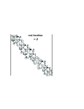
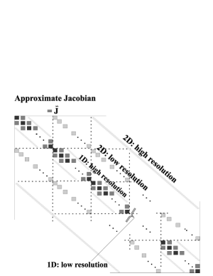
Figure 1: The real Jacobian matrix ($\rm{{J}}$, left) and an approximate Jacobian matrix ($\rm{\tilde{J}}$, right). In $\rm{\tilde{J}}$ we have displayed the entries (blocks) that correspond to low and high spacial resolution in one and two dimensions.

3 Highly compressed low Mach flows: an iterative non-linear preconditioned Newton solver

Assume we are given a two-dimensional nonlinear vector equation of the form:

$$\frac{\partial q}{\partial t}+\frac{\partial F(q)}{\partial x}+\frac{\partial G(q)}{\partial y}=f,$$ (25)

where $q,F,G,f$ denote the vector of variables, their momentum flux both in x and y-directions and a source function, respectively.
Define the residual $\mathrm{d(q)}$ and look for the vector $\mathrm{q},$ such that $\mathrm{d(q)}=0$, i.e.,

$$d(q)=f-\left[\frac{\partial q}{\partial t}+\frac{\partial F(q)}{\partial x}+\frac{\partial G(q)}{\partial y}\right]=0.$$ (26)

In the case of a single one-dimensional nonlinear function $\mathcal{F}(x)=0$, the zeros can be found using the Newton iteration method:

$$x^{\mathrm{i+1}}=x^{\mathrm{i}}-\frac{\mathcal{F}}{\dot{\mathcal{F}}},$$ (27)

where $\dot{\mathcal{F}}(x^{\mathrm{i}})=\frac{\partial\mathcal{F}}{\partial x}|_{\mathrm{x=x^{\mathrm{i}}}}$ and “i” denotes the iteration number. When applying this approach to a general system of equations such as Eq. (25), we have then to perform the following replacements:

$$\left.\begin{array}[]{lll}x&\mapsto&q,\\ \mathcal{F}(x)&\mapsto&d(q)\\ \dot{\mathcal{F}}&\mapsto&J,\end{array}\right\}\begin{array}[]{ll}&\\ \Rightarrow&q^{\mathrm{i+1}}=q^{\mathrm{i}}-\mathrm{J^{-1}}{\mathrm{d}}\\ &\end{array}$$ (28)

where J is the Jacobian matrix defined as: $J=\frac{\partial R}{\partial q}.$
Defining $\mu=q^{\mathrm{i+1}}-q^{\mathrm{i}}$, we may re-write Eq. (28) as:

$$\rm{J\,\mu=d},$$ (29)

where “d” is calculated using arbitrary high spatial and temporal accuracies.
The matrix Equation (29) is said to be:

$$\left\{\begin{array}[]{lll}\textrm{Linear\,:}&\mathrm{if}&\mathrm{d=d(q^{\mathrm{n}})}\\ \textrm{Otherwise \,:}&\mathrm{if}&\mathrm{d=d(q^{\mathrm{i}})}.\\ \end{array}\right.$$ (30)

While in the first case, one need to invert the Jacobian once per time step, in the second case however, several iterations per time step might be required to recover the nonlinearity of the solution. The calculation may become prohibitively expensive, if the Jacobian to be inverted corresponds to a system of equation in multi-dimensions to be solved with high spatial and temporal accuracies.
The idea of preconditioning is to calculate the defect “d” as proposed by the physical problem (e.g., with very high resolution), whereas the Jacobian is replaced then by an approximate matrix $\mathrm{\tilde{A}}$ of the following properties:

• $\mathrm{\tilde{A}}$ is easier to invert than J,

• $\mathrm{\tilde{A}}$ and J are similar and share the same spectral properties.

While the first property is easy to fulfill, the second one is in general an effort-demanding issue. It states that the preconditioning $\mathrm{\tilde{A}}$ should differ only slightly from the Jacobian if trivial replacement to be avoided. therefore, given the matrix $\mathrm{\tilde{A}}$, the solution procedure would run as follows:

1. Compute the defect “d”.

2. Use the matrix equation: $\mathrm{\tilde{A}}\,\mu=\,d.$ to solve for $\mu.$

3. Update: $q^{\mathrm{i+1}}=q^{\mathrm{i}}+\mu,$ re-calculate “d” and $\mathrm{\tilde{A}}$, respectively.

4. The procedure (2) and (3) should be repeated until $\max(|d|)$ is smaller than a number $\epsilon$, where the maximum runs over all the elements of “d”.

The fundamental question to be addressed still is: how to construct a robust preconditioner $\mathrm{\tilde{A}}$ that is capable of modeling low-Mach number flows efficiently, but still easy to invert?
In this construction, two essential constrains should be taken into account:

• A conservative first order spatial discretization of the Navier-Stokes equations generally yields a Jacobian matrix of penta-diagonal block form as depicted in Figure (1).

• The gradients of the thermal pressure are dominant, so that the pressure-related terms must be treated simultaneously.

In order to clarify these points, we re-write the matrix Equation (29) at an arbitrary grid point (j,k) in the following block form:

$$\begin{array}[]{lll}&{\hskip 8.5359pt}\overline{S}^{\mathrm{y}}_{\mathrm{j,k}}{\mu}_{\mathrm{j,k+1}}&\\ +\underline{S}^{\mathrm{x}}_{\mathrm{j,k}}{\mu}_{\mathrm{j-1,k}}&+{D}^{\mathrm{mod}}_{\mathrm{j,k}}{\mu}_{\mathrm{j,k}}&+\overline{S}^{\mathrm{x}}_{\mathrm{j,k}}{\mu}_{\mathrm{j+1,k}}=d_{\mathrm{j,k}}\\ &+\underline{S}^{\mathrm{y}}_{\mathrm{j,k}}{\mu}_{\mathrm{j,k-1}},&\end{array}$$ (31)

where $\underline{S}^{\mathrm{x,y}},\leavevmode\nobreak\ \overline{S}^{\mathrm{x,y}}$ denote the sub and super-diagonal block matrices and ${D}^{\mathrm{mod}}=I/{\delta t}+{D}^{\mathrm{x}}+{D}^{\mathrm{y}}$ the diagonal block matrices, respectively.
While this block structure is best suited for using the one-colored or multi-colored line Gauss-Seidel iterative method, test calculations have shown however, that these iterative methods may stagnate or they may even diverge if the flow is of low mach number type. The reason for this behaviour is that most iterative methods rely either on partial updating of the variables or on the dimensional splitting. These, however, are considered to be inefficient methods or they may even stagnate, if the system of equations to be solved are of elliptic type, such as the Possion equations.

One way to take the multi-dimensional variations of the pressure all at one time is to spatial-factorize the Jacobian into sub-matrices, such that the resulting multiplication results in a good approximation of the original Jacobian, i.e.,

$$\rm{J\mapsto\Pi_{\mathrm{lm}}\tilde{A}_{\mathrm{l}}\tilde{A}_{\mathrm{m}}}.$$ (32)

The advantages of this method is that the gradients of the pressure in all direction are incorporated in the matrix $\tilde{A}$. Furthermore, the right hand side, i.e., the defect is updated only after all matrices $\tilde{A}_{\mathrm{m}}$ are fully inverted. We note that this preconditioner can be used even as a direct solver as long as time-dependent solutions are concerned. To clarify this procedure, we rewrite Equation (25) in the finite space as follows:

$$\rm{\frac{\delta q}{\delta t}+\frac{\Delta_{x}F^{\mathrm{n+1}}}{\Delta x}+\frac{\Delta_{y}G^{\mathrm{n+1}}}{\Delta y}=0,}$$ (33)

where $\rm{\delta q=q^{\mathrm{n+1}}-q^{\mathrm{n}}}(\mu)$ and $\Delta_{\mathrm{x,y}}$ are space difference operators.
We may expand $\rm{F^{\mathrm{n+1}}}$ and $\rm{G^{\mathrm{n+1}}}$ around their values at the old time levels as follows:

$$\mathrm{F}^{\mathrm{n+1}}=\mathrm{F}^{\mathrm{n}}+{\delta t}\left(\frac{\partial F}{\partial t}\right)^{\mathrm{n}}+\mathcal{O}(\delta t)^{2}=\mathrm{F}^{\mathrm{n}}+{\delta t}\left(\frac{\partial F}{\partial q}\right)^{n}\left(\frac{\partial q}{\partial t}\right)^{\mathrm{n}}+\mathcal{O}(\delta t)^{2}\mapsto\mathrm{F}^{\mathrm{n}}+{\delta t}A^{n}\left(\frac{\delta q}{\delta t}\right)^{\mathrm{n}}+\mathcal{O}(\delta t)^{2}.$$

Equivalently,

$$\mathrm{F}^{\mathrm{n+1}}=\mathrm{F}^{\mathrm{n}}+A^{n}\delta q+\mathcal{O}(\delta t)^{2},$$

$$\mathrm{G}^{\mathrm{n+1}}=\mathrm{G}^{\mathrm{n}}+B^{n}\delta q+\mathcal{O}(\delta t)^{2},$$ (34)

Substituting these expressions into Equation (33), we obtain:

$$\rm{\left[\frac{I}{\delta t}+L_{\mathrm{x}}A^{n}+L_{\mathrm{y}}B^{n}+\mathcal{O}(\delta t)^{2}\right]\delta q=L_{\mathrm{x}}F^{n}+L_{\mathrm{y}}G^{n},}$$ (35)

where $\rm{L_{\mathrm{x}},L_{\mathrm{y}}}$ denote the differential operators in x and y-directions, respectively. We may replace Equation (35) by the following approximation:

$$\rm{\left[\frac{I}{\delta t}+L_{\mathrm{x}}A^{n}\right]\left[I+\delta t\,L_{\mathrm{y}}B^{n}\right]\delta q=L_{\mathrm{x}}F^{n}+L_{\mathrm{y}}G^{n},}$$ (36)

This replacement induces an error which is proportional to : $\delta t\,L_{\mathrm{x}}\,L_{\mathrm{y}}+\mathcal{O}(\delta t)^{2}.$ This error may diminish for steady conserved fluxes, but may diverge for time-dependent solutions if the time steps are large. The latter disadvantage is relaxed by the physical consistency requirement, that small time steps are to be used if the the sought solutions are time-dependent.
The matrix Equation (36) can be re-written in the following compact form:

$$\mathrm{\tilde{A}_{\mathrm{x}}}\,\mathrm{\tilde{A}_{\mathrm{y}}}\mu=\mathrm{d},$$ (37)

where $\mathrm{\tilde{A}_{\mathrm{x}}}=\frac{I}{\delta t}+L_{\mathrm{x}}A^{n}$ and $\mathrm{\tilde{A}_{\mathrm{y}}}=\frac{I}{\delta t}+L_{\mathrm{y}}B^{n}.$

Applying this factorization within a non-linear iterative solution procedure, the solution procedure would run as follows:

1. Compute the defect $\rm{d=d(q^{\mathrm{i}},q^{\mathrm{n}})}$ at each grid point using the best available spatial and temporal accuracies.

2. Solve the matrix equation: $\mathrm{\tilde{A}_{\mathrm{x}}}\delta q^{*}=d,$ to obtain $\delta q^{*}$.

3. Solve the matrix equation: $\mathrm{\tilde{A}_{\mathrm{y}}}\delta q=\delta q^{*}$ to obtain $\delta q.$

4. Update q: $q^{\mathrm{i+1}}=q^{\mathrm{i}}+\delta q$ and subsequently the defect d.

5. Perform a convergence check to verify if $\max(|d|)<\epsilon$. If not, then repeat the algorithmic steps 1-4 repeatedly.

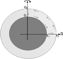
Figure 2: Two concentric spheres: the inner sphere has a radius $R_{1}$ and rotates with angular velocity $\Omega_{1}$ whereas the outer one has the radius $R_{2}$ and rotates with $\Omega_{2}$.

4 Taylor-Couette flows between two concentric spheres

Large scale motions of gas in stellar spherical shells are controlled by the imbalance of energies, namely between the potential, thermal, rotational and magnetic energies. It is generally accepted that rotation deforms surfaces of constant pressure, but has only indirect influence on surfaces of constant temperatures. The resulting baroclinicity is unbalanced and derives large scale meridional circulation (Sweet, 1950). On the local scale, these flows are in general convectively unstable, hence governed by convective turbulence. Such combined motions are observationally evident in the solar convective zone.
In the laboratory, spherical Couette flows between two rotating spheres are considered to be similar to rotating stellar envelopes. In the case of fast rotation, the flow is a combination of primary azimuthal rotations and a secondary meridional circulation induced by Ekman pumping (Greenspan, 1968). Here the flow is controlled by two parameters: The Reynolds number and the gap width between the two spheres. The Reynolds number for this configuration is defined as:

$$\mathrm{Re=\frac{|\Delta\Omega|R_{1}|\Delta R|}{\nu},}=\frac{|\Omega_{2}-\Omega_{1}|\leavevmode\nobreak\ R_{1}\leavevmode\nobreak\ |R_{2}-R_{1}|}{\nu},$$ (38)

where $R_{1,2},\leavevmode\nobreak\ \Omega_{1,2}\mathrm{\leavevmode\nobreak\ \leavevmode\nobreak\ and\leavevmode\nobreak\ \leavevmode\nobreak\ }\nu$ are the inner and outer radii, the angular frequency of the inner and outer sphere and the viscosity coefficient, respectively (Figure 2).
The number of rotationally-induced fluid vortices and transition to turbulence in Couette flows depend on how large the Reynolds number is as well on the width $\delta$ of the gap between the two spheres. For example, for $\mathrm{Re>460}$ and $\delta=1.006$ Couette flows have been verified to become turbulent (Gertsenshtein et al., 2001).

In applying our solver to Couette flows between two-concentric spheres, the following parameters have been used: $\Omega_{1}=3,\leavevmode\nobreak\ \leavevmode\nobreak\ \Omega_{2}=0,\leavevmode\nobreak\ \leavevmode\nobreak\ R_{1}=1,\leavevmode\nobreak\ \leavevmode\nobreak\ R_{1}=1.25$ and a viscosity coefficient $\nu=0.005$ (see Figure 3).
The domain of calculation is limited to the first quadrant $[1\leq R\leq 1.25]\times[0\leq\theta\leq\pi/2].$ Along the equator and polar axis reflecting boundary conditions have been imposed, whereas the outer and inner boundaries are set to be rigid with zero material flux across them.

In order to test the capability of the solver to deal with low Mach number flows, we have systematically increased the temperature from 10 up to one million, which corresponds to a reduction of the Mach number by at least two orders of magnitude.
Our results, partially displayed in Figure (3), indicate that AFM as a preconditiong in combination with the defect-correction Newton iteration is indeed capable of modelling weakly incompressible flows down to Mach number $\mathcal{M}\approx 10^{-3}$.

Figure 3: Taylor-Couette flows: the inner sphere has a radius $\mathrm{R_{1}=1}$ and rotates with $\Omega_{1}=3$, whereas the outer sphere has a radius $\mathrm{R_{1}=1.2}$ and $\Omega_{1}=0$. The flow has the constant viscosity coefficient $\alpha=0.005$. The Mach number is set to decrease systematically by increasing the temperature from $\mathrm{T=10^{2}}$ up to $\mathrm{T=10^{6}}$. This corresponds to a reduction of the Mach number by two orders of magnitude. The right panel shows the corresponding time-evolution of the time step size in units of Courant number.

5 Summary

In this paper we have shown that weakly incompressible flows in astrophysics are actually highly compressible low Mach number flows in which the pressure plays a vital role in dictating the fluid motions. Therefore, these flows can be well-treated using a robust compressible numerical solver in combination with a sophisticated treatment of the pressure terms.
However, as the sound wave crossing time in low Mach number flows is extremely short relative to the hydrodynamical time scale, we have concluded that time-explicit methods are not suited.
On the other hand, projection methods based on Possion-like solvers for the pressure violates the conservative formulation of the hydrodynamical equations, namely the entropy principle and therefore the monotonicity character of the scheme.

Our conclusion is that the set of hydrodynamical equations describing the time-evolution of compressible low Mach number flows should be solved using an implicit robust solver. Our numerical studies show that nonlinear Newton-type solvers in combination with the defect-correction iteration procedure and using the Approximate Factorization Method (AFM) as preconditioning is best suited for treating such flows. Unlike the classical non-direct methods that rely on dimensional splitting and/or partial updating, e.g., ADI and Line-Gauss-Seidel, the AFM is based on factorizing the Jacobian matrix and subsequently updating the variable in all directions simultaneously. Similar to the treatments of the pseudo-pressure in incompressible flows, the pressure gradients in low Mach number flows do not accept dimensional splitting even when it is applied within the preconditioning only.