Offdiagonal complexity: A computationally quick network complexity measure. Application to protein networks and cell division

Abstract

Many complex biological, social, and economical networks show topologies drastically differing from random graphs. But, what is a complex network, i.e. how can one quantify the complexity of a graph? Here the Offdiagonal Complexity (OdC), a new, and computationally cheap, measure of complexity is defined, based on the node-node link cross-distribution, whose nondiagonal elements characterize the graph structure beyond link distribution, cluster coefficient and average path length. The OdC apporach is applied to the Helicobacter pylori protein interaction network and randomly rewired surrogates thereof. In addition, OdC is used to characterize the spatial complexity of cell aggregates. We investigate the earliest embryo development states of Caenorhabditis elegans. The development states of the premorphogenetic phase are represented by symmetric binary-valued cell connection matrices with dimension growing from 4 to 385. These matrices can be interpreted as adjacency matrix of an undirected graph, or network. The OdC approach allows to describe quantitatively the complexity of the cell aggregate geometry.

25.1 Complex networks

From a series of seminal papers (Watts & Strogatz wattsstrogatz , Barabasi & Albert barabasialbert ; albertbarabasi ; barabasilinked , Dorogovtsev & Mendes doromend , Newman newman , see also bornschu for an overview) since 1999, small-world and scale-free networks have been a hot topic of investigation in a broad range of systems and disciplines.
Metabolic and other biological networks, collaboration networks, www, internet, etc., have in common that the distribution of link degrees follows a power law, and thus has no inherent scale. Such networks are termed ‘scale-free networks’. Compared to random graphs, which have a Poisson link distribution and thus a characteristic scale, they share a lot of different properties, especially a high clustering coefficient, and a short average path length. However, the question of complexity of a graph still is in its infancies. A ‘blind’ application of other complexity measures (as for binary sequences or computer programs) does not account for the special properties shared by graphs and especially scale-free graphs as they appear in biological and social networks.

Mathematically, a graph (or synonymously in this context, a network) is defined by a (nonempty) set of nodes, a set of edges (or links), and a map that assigns two nodes (the “end nodes” of a link) to each link. In a computer, a graph may be represented either by a list of links, represented by the pairs of nodes, or equivalently, by its adjacency matrix $a_{ij}$ whose entries are 1 (0) if nodes $i,j$ are connected (disconnected). Useful generalizations are weighted graphs, where the restriction of $a_{ij}$ is relaxed from binary values to (unsually nonnegative) integer or real values (e.g. resistor values, travel distances, interaction coupling), and directed graphs, where $a_{ij}$ no longer needs to be symmetric, and the link from $i$ to $j$ and the link from $j$ to $i$ can exist independently (e.g. links between webpages, or scientific citations). In this chapter the discussion will be kept limited to binary undirected graphs.

25.2 Complexity measures in biology

In biological sciences, the evolution of life is studied in detail and at large; and it is observed qualitatively that evolution creates, on average, organisms of increasing complexity. If one wants to quantify an increase of complexity, one has to define siutable complexity measures. In some sense, the number of cells may be an indicator, but quantifies rather body size than complexity. Instead one may observe the number of organelles, the size of the metabolic network, the behavioural complexity of social organisms, or similar properties. To have a time series of the complexity distribution of all organisms during evolution on earth, would be highly interesting for the test of models of evolution, speciation and extinctions. But apart from such academic questions, there are many areas of practical use of complexity measures in biology and medicine, as the complexity of morphological structures, cell aggregates, metabolic or genetic networks, or neural connectivities.

25.3 Other complexity measures

For text strings (as computer programs, or DNA) there are common complexity measures in theoretical computer science, such as Kolmogorov complexity (and the related Lempel-Ziv complexity and algorithmic information content AIC) gellmannLloyd . For example, AIC is defined by the length of the shortest program generating the string. For random structures, thus also for random graphs, these measures indicate high complexity. A distinction of complex structured (but still partly random) structures from completely random ones usually is prohibitive for this class of measures. For this reason, measures of effective complexity gellmann have been discussed; usually these are defined as an entropy (or description length) of “a concise description of a set of the entity’s regularities” gellmann . Here we are mainly interested in this second class, and straightforwardly one would try to apply existing measures, e.g., to the link list or to the adjacency matrix. However, mathematically it is not straightforward to apply these text string based measures to graphs, as there is no unique way to map a graph onto a text string.

Thus one desires to use complexity measures that are defined directly for graphs. Two classical measures are known from graph theory; graph thickness and coloring number have a low “resolution” and their relevance for real networks is not clear. Two new complexity measures recently have been proposed for graphs, Medium Articulation wilhelm for weighted graphs (as they appear in foodwebs) and a measure for directed graphs by Meyer-Ortmanns meyer based on the network motif concept alon_motif ). Unfortunately, the latter two complexity measures are computationally quite costly. A computational complexity approach has been defined by Machta and Machta machtamachta as computational depth of an ensemble of graphs (e.g. small-world, scalefree, lattice). It is defined as the number of processing time steps a large parallel computer (with an unlimited number of processors) would need to generate a representative member of that graph ensemble. Unlike other approaches, it does not assign single complexity values to each graph, and again is nontrivial to compute.

Table 25.1 gives a qualitative assessment of the behaviour of some of the mentioned complexity measures for lattices in 2D and 3D, complex and random structures. Note that especially the ability to distinguish nonrandom complex structures from pure randomness differs between the approaches. Hence, a simpler estimator of graph complexity is desired, and one possible approach, the Offdiagonal Complexity, is proposed here. A striking observation of the node-node link correlation matrices of complex networks claussenddhs03 ; claussendd is, that entries are more evenly spread among the offdiagonals, compared to both regular lattices and random graphs. This can now be used to define a complexity measure, for undirected graphs claussenddhs03 ; claussendd .

This chapter is organized as follows. In Sec. 25.4 OdC is defined and illustrated with an example. Sections 25.5 and 25.6 investigate the application of OdC to two quite different biological problems: a protein interaction network, compared with randomized surrogates, and a temporal sequence of spatial cell adjacency during early Caenorhabditis elegans development, quantifying the temporal increase of complexity.

Table 25.1: Qualitative assessment of various complexity measures.

	2D, 3D	complex structures	random structures
AIC, Kolmogorov	$o(1)$	large	maximal
effective complexity	$o(1)$	large	$o(1)$
coloring number	2, 2	$\simeq 3-4$	$\simeq 3-4$
graph thickness	2, $N^{1/3}$	$\simeq 2-5$	$\simeq 3-4$
motif count	$o(1)$	large	large
Machta	$o(1)$	large	$o(1)$
OdC	0	large	low

25.4 Definition of the Offdiagonal Complexity (OdC)

Definition (Offdiagonal complexity). Let $g_{ij}$ be the adjacency matrix of a graph with $N$ nodes, i.e., $g_{ij}=1$ if nodes $i$ and $j$ are connected, else $g_{ij}=0$.

(i)

For each node $i$ of the graph, let $l(i)$ be the node degree, i.e. the number of edges (links),

$$l(i):=\sum_{j=0}^{N-1}g_{ij}$$ (25.1)

(ii)

Let $c_{mn}$ be the number of edges between al pairs of nodes $i$ and $j$, with node degrees $m=l(i)$, $n=l(j)$ with $l(j)\geq l(i)$ (ordered pairs), i.e.,

$$c_{mn}:=\sum_{j=0}^{N-1}\sum_{j=0}^{N-1}g_{ij}\delta_{m,l(i)}\delta_{n,l(j)}H(l(i)-l(j)).$$ (25.2)

Here $\delta$ is the Kronecker symbol and $H(x)=1$ for $x\leq 0$ and $H(x)=0$ for $x>0$. Due to the pair odering, the matrix $c_{mn}$ has entries only on the main diagonal and above. Thus, $c_{mn}$ is a (not normalized) node-node link correlation matrix.

(iii)

Summation over the minor diagonals, or offdiagonals, i. e. all pairs with same $k_{i}-k_{j}$ up to $k_{\rm max}=\min_{i}\{l(i)\}$, and normalization, gives us

$$\tilde{a}_{k}=\sum_{i=0}^{k_{\rm max}-k}c_{i,k+i},~{}~{}~{}~{}~{}~{}~{}~{}~{}~{}A:=\sum_{k0}^{k_{\rm max}}\tilde{a}_{k},~{}~{}~{}~{}~{}~{}~{}~{}~{}~{}\forall_{k}a_{k}:=\tilde{a}_{k}/A.$$ (25.3)

(iv)

Then OdC is defined as an entropy measure on this normalized distributions (here it is understood that $0\ln(0)=0$),

$${\rm OdC}=-\sum_{k=0}^{k_{\rm max}}a_{k}\ln a_{k}.$$ (25.4)

Examples: For a d-dimensional orthogonal lattice, all nodes have degree $2d$, and the node-node link correlation matrix has only one nonzero entry at row $2d$ and column $2d$. For a fully connected graph, the single entry is at row $N$ and column $N$. Obviously, for regular graphs (where all node have a fixed degree $k$) OdC=0 holds in general.

OdC is an approximative complexity estimator that takes as values zero for a regular lattice, zero for a fully connected graph, low values for a random graph, and higher values for ‘apparently complex’ structures. One main advantage is that it does not involve costly (high-order or NP-complete) computations.

25.4.1 Illustration with a spatial network

A spatial hierarchical network emerging from a self-organizing process has recently been introduced by Sakaguchi sakaguchi , as shown in Fig. 25.1a. This snapshot example is now taken to illustrate how the node-node link correlation matrix and the OdC entropy are modified under a random reshuffling of links.

(a) Self-organized

structure by Sakaguchi

$k$	1	2	3	4	5	6	7	8
$\#k$	10	8	6	4	1	0	1	1

Link correlation matrix:
0 0 1 2 0 0 2 5 3 2 2 2 0 3 1 $\ddots$ 3 8 0 0 0 1 $\ddots$ 5 1 1 0 1 0 $\ddots$ 3 0 0 1 2 $\ddots$ 4 0 0 0 $\ddots$ 0 0 0 $\ddots$ 7 0 $\ddots$ 4 $\ddots$ 11 7
The vector of diagonal sums is
(7,11,4,7,0,4,3,5).
Resulting entropy: ${\rm OdC}=1.858622$

(b) Same network, links partly

randomized (1 move/node)

$k$	1	2	3	4	5	6	7	8
$\#k$	8	7	8	5	2	1	0	0

Link correlation matrix:

0	1	4	0	2	1	0	0
	0	7	5	1	0	0	0	$\ddots$
		2	4	4	1	0	0	$\ddots$	0
			3	2	3	0	0	$\ddots$	0
				0	1	0	0	$\ddots$	1
					0	0	0	$\ddots$	2
						0	0	$\ddots$	2
							0	$\ddots$	16
								$\ddots$	15
									5

The vector of diagonal sums is

(5,15,16,2,2,1,0,0).

Resulting entropy: ${\rm OdC}=1.376939$

The random reshuffling lowers the OdC entropy away from

${\rm OdC}_{max}=2.550838$.

Figure 25.1: (a) Self- organized structure by Sakaguchi. (b) Randomly rewired network.

25.5 Application to the Helicobacter pylori protein interaction graph and reshuffling to a random graph

To demonstrate that OdC can distinguish between random graphs and complex networks, the Helicobacter pylori protein interaction graph helico_dat has been chosen. For different rewiring probabilities $p$ and $10^{2}$ realizations each, the links have been reshuffled, ending up with a random graph for $p=1$. As can be seen in Fig. 25.2, rewiring in any case lowers the Offdiagonal Complexity.

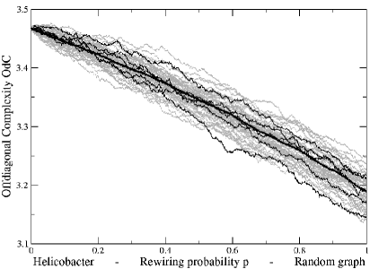
Figure 25.2: OdC for random reshufflings of the Helicobacter pylori network (left, $p=0$) up to a rewiring probability of $p=1$ (right). The bold line shows the average, five OdC trajectories along a rewiring path are shown for illustration (thin lines).

25.6 Application to spatial cell division networks

The tiny (1mm) nematode worm Caenorhabditis elegans looks like a quite primitive organism, but nevertheless has a nervous system, muscles, thus shares functional organs with higher-developed animals. More important, it shows a morphogenetic process from a single-cell egg thorugh morphogenesis to an adult worm. Towards an understanding of the genetic mechanisms of the cell division cycle in general, C.elegans has become one of the genetically best studied animals. Despite that, little is known (in the sense of a dynamical model) how the cell divison and spatial reorganization takes place. Not even the spatial organization of cells during morphogenesis is well described.

25.6.1 Early development of C.elegans

The earliest embryo development states of Caenorhabditis elegans have been recorded experimentally and described quantitatively recently akraemerphd . The cell division development have been described in simplicial spaces, and the cell division operations are described by operators in finite linear spaces simplicial .

25.6.2 Topological structure during premorphogenesis

The premorphogenetic phase of development runs until the embryo reaches a state of about 385 cells. The detailed division times and spatial cell movement trajectories follow with high precision a mechanism prescribed in the genetic program. While many of the genetic mechanisms are known especially for C.elegans, we are a long way towards a mathematical modelling of the cell divison and spatial organization directly from the genome. Thus it is still desired to develop mathematical models for this spatiotemporal process, and to compare it with quantitative experimental data.
With good reliability the cell adjacency is known experimentally akraemerphd ; simplicial in a number of intermediate steps, which in the remainder we called cell states. Here we focus on the adjacency matrices of the cells describing each intermediate state between cell divisions and cell migrations, and investigate the complexity of neighborhood relations.

25.6.3 Increasing complexity of C.elegans states

The result for 28 state matrices are shown in Fig. 25.3. The dashed line shows the supremum value $(-\ln N)$ a graph of the same size could reach, despite the fact that due to combinatorical reasons this supremum is not necessarily always reached.
The moderate decay in the last two states may be due to the fact that (at least for Poisson-like link distributions) the summation implies some self-averaging if one wants to compare networks of different size. One way to avoid this problem is to define the complexity measure from all $k_{\rm max}\cdot(k_{\rm max}-1)$ entries,

$${\rm FOdC}:=-\sum_{i=0}^{k_{\rm max}}\sum_{j=i}^{k_{\rm max}}c_{ij}\ln(c_{ij}).$$ (25.5)

This can be called Full Offdiagonal Complexity, as the full set of matrix entries is taken into account. The result for FOdC is shown in Fig. 25.3.

Figure 25.3: Left: Offdiagonal complexity of the network states. The dashed line shows the maximal complexity a graph of same number of nodes could reach. Right: Full Offdiagonal complexity. Here all possible pairs of nodes contribute to the complexity.

25.6.4 Saturation for large network size

As expected, the complexity of the spatial cell structure increases along the first premorphogenetic phase. Compared to the maximal possible complexity that could be reached by a graph of same number of node degrees (but not for a three-dimensional cell complex) the complexity, as measured by OdC, saturates. This has a straightforward explanation: The limiting case of a large homogeneous cell agglomerate would end up with roughly two classes of cells (at surface and within bulk) and thus three classes of neighborhood pairs: bulk-bulk, bulk-surface and surface-surface (see Fig. 25.4). As the coordination numbers within bulk and surface fluctuate, this effectively delimits the growth of possible different neighborhood geometries. After initial growth, FOdC resolves fluctuations corresponding to the effect of alternating cell division and spatial reorganization.

   

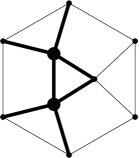
Figure 25.4: Intuitive explanation of saturation for large homogeneous spatial networks. From left to right: Bulk-bulk, bulk-surface, and surface-surface are the typical pairs of node degrees. For large cell aggregates, surface and bulk cells are more homogeneously, i.e. the variation of the neighborhood degree decreases.

25.7 Conclusions and Outlook

A new complexity measure for graphs and networks has been proposed. Contrary to other approaches, it can be applied to undirected binary graphs. The motivation of its definition is twofold: One observation is that the binning of link distributions is problematic for small networks. Herefrom the second observation is that if one uses instead of the (plain) entropy of link distribution, which is unsignificant for scale-free networks, a “biased link entropy”, it has an extremum where the exponent of the power law is met.
The central idea of OdC is to apply an entropy measure to the link correlation matrix, after summation over the offdiagonals. This allows for a quantitative, yet still approximative, measure of complexity. OdC roughly is ‘hierarchy sensitive’ and has the main advantage of being computationally not costly.

References

- [1] D.J. Watts and S.H. Strogatz, Nature 393, 440-442 (1998).
- [2] A.L.Barabasi and R. Albert, Science, 286, 509-512 (1999).
- [3] R. Albert, A.-L. Barabasi, Statistical mechanics of complex networks, Reviews of Modern Physics 74, 47-97 (2002).
- [4] A.-L. Barabasi, Linked, Plume Books, New York (2003).
- [5] S.N. Dorogovtsev, J.F.F. Mendes, Evolution of networks, Adv. Phys. 51, 1079 (2002)
- [6] M. E. J. Newman, The structure and function of complex networks, cond-mat/0303516, SIAM Review 45, 167-256 (2003).
- [7] S. Bornholdt, H.-G. Schuster (eds.), Handbook of Graphs and Networks, Wiley-VCH, Berlin (2002).
- [8] M. Gell-Mann, S. Lloyd. Information measures, effective complexity, and total information. Complexity 2(1), 44-52 (1996).
- [9] M. Gell-Mann. What is complexity? Complexity 1(1), 16-19 (1995).
- [10] T. Wilhelm, An elementary dynamic model for non-binary food webs, Ecol. Model. 168, 145-152. (2003).
- [11] H. Meyer-Ortmanns, Functional Complexity Measure for Networks, Physica A 337, 679-690 (2004).
- [12] R. Milo, S. Shen-Orr, S. Itzkovitz, N. Kashtan, D. Chklovskii, and U. Alon, Network Motifs: Simple Building Blocks of Complex Networks, Science 298, 824-827 (2002).
- [13] B. Machta and J. Machta, Parallel dynamics and computational complexity of network growth models, Phys. Rev. E 71, 026704 (2005).
- [14] Jens Christian Claussen, AKSOE 3.10, Verhandl. Deutsche Phys. Ges. Regensburg (2004). (Extended version of unpublished talk draft, Nov. 11, 2003).
- [15] J.C. Claussen, Characterization of networks by the Offdiagonal Complexity, Physica A 375, 365-373 (2007)
- [16] Hidetsugu Sakaguchi, Self-organization of hierarchical structures in nonlocally coupled replicator models, Phys. Lett. A 313, 188-191 (2003).
-
[17]
Helicobacter pylori data,
http://www.cosin.org/,http://www.helico.com/ -
[18]
A. Krämer,
PhD thesis,
Kiel 2002,
http://e-diss.uni-kiel.de/diss_617/ - [19] A. Krämer, unpublished; A. Betten and D. Betten, The proper linear spaces on 17 points, Discrete Applied Mathematics, 95, 83-108 (1999).