Anyonic Loops in Three Dimensional Spin liquid and Chiral Spin Liquid

Abstract

We established a large class of exactly soluble spin liquids and chiral spin liquids on three dimensional helix lattices by introducing Kitaev-type’s spin coupling. In the chiral spin liquids, exact stable ground states with spontaneous breaking of the time reversal symmetry are found. The fractionalized loop excitations in both the spin and chiral spin liquids obey non-abelian statistics. We characterize this kind of statistics by non-abelian Berry phase and quantum algebra relation. The topological correlation of loops is independent of local order parameter and it measures the intrinsic global quantum entanglement of degenerate ground states.

I Introduction

Topological order of condensed matter system is the cornerstone of topological quantum computationdas . The topologically ordered system have degenerated ground states which depend on the topology instead of symmetry. This degeneracy of ground state is robust against any local perturbation due to the gap between ground state and excited stateswen . An interesting application of topological stablizer quantum codes is implemented in Kitaev’s toric code modeltoric . A topological color codes with quantum error-correcting capabilities is developed latercolor , this model removes the need for selective addressing.

There are different ways to perform quantum computation in use of topologically ordered states. Usually the quantum gate or unitary transformation are implemented by brading quasiparticles. The transversal implementation of quantum gate provides us another way of topological quantum computation without braidingnobraid , in which the stablizer color codes is achieved in a 3-dimensional lattice model. While we focus on the braiding of loop quasiparticles in 3-dimensional spin liquid and chiral spin liuid in this paper.

We established the 3-dimenisonal spin liquids by generalizing Kitaev’s two dimensional spin model. Kitaev’s spin model on honeycomb lattice has a highly degenerate ground statekitaev . Abelian anyons and non-abelian anyons emerge in the background of short range spin liquid. These anyonic excitations obey exotic statistics. Quantum computation is based on anyon braiding. During the braiding operation, anyons interact with one another only by encircling a topological nontrivial cycle. A proposal of the experimental operation of anyon braiding in Kitaev honeycomb model has been provided by use of ultracold atoms trapped in optical latticescwzhang , however there is some controversal on the details of this experimental proposal08014620 .

Another most promising candidate of non-abelian anyons may be realized in fractional quantum Hall states with $\nu=5/2$read ; xia . The fractional quantum Hall states break parity and time-reversal symmetry since fractional quantum Hall occurs in the presence of a strong magnetic field. Quantum information is stored in different fusion channels of non-abelian anyonsdas . For two $\sigma$ quasiparticles following fusion rule $\sigma\cdot\sigma\sim{\textbf{1}+\psi}$, if fusion outcome is 1, we define the qubit as state $|0\rangle$. When fusion outcome is $\psi$, the state of the qubit is $|1\rangle$. We may use $2n$ antidots at which quasiholes are pinned to construct $n$ qubits.

Non-abelian anyons also arise from other two dimensional systems, such as $Sr_{2}RuO_{4}$. In this $p+ip$ superconductor, the half-quantum vortices with flux $hc/2e$ exhibit non-abelian statisticsdas2 . Spin-$1/2$ chiral spin liquid states proposed by Kalmeyer and Laughlin possess fractionalized excitationskalmeyer . This kind of non-abelian anyons appears in 2D solvable spin models which are generalization of Kitaev honeycomb modelyao yangsun . These anyons are point quasiparticles confined in two dimensions. The main disadvantage of two dimensional system is that the expectation value of topological symmetry operators vanishes at finite temperature. This makes the topological memory thermally fragilealicki ortiz .

Since most physical materials in nature are three dimensional, anyonic excitations most likely exist in three dimensions. One clue comes from a three dimensional exactly solvable spin model constructed by generalizing Kitaev’s toric code to cubic latticehamma , in which the topological order of its ground state is characterized by string net condensation as well as membrane condensation. The string net and membrane condensation also appear in another exactly solvable spin modelbrane , which is constructed on a general 3-complex embedded in a closed and connected base manifold in three dimension. Its ground state degeneracy depends on the homology of the 3-manifold.

To establish three dimensional chiral spin liquid, we start from a different way to search for anyons in three dimensions by generalizing Kitaev honeycomb lattice model. Our interest focuses mainly on nontrivial loop excitations. Loops confined in two dimensions have no non-trivial entanglement without cutting each other. It is in three dimensions that loops demonstrate much interesting statistical phenomena without breaking topological constraint. There is a loop braiding group for the statistics of unknotted, unlinked closed stringsbaez . For links consisting of many entangled knots, their non-abelian statistics is closely related to the monodromy matrix in conformal field theory witten ; ms . Quantum loop gas applied to topological quantum computation is under rapid developingloops .

There were some theoretical investigations on three dimensional chiral spin liquid based on effective field theorylibby . However, no exact three dimensional chiral spin liquid is found so far to the authors’ knowledge. We established a large class of exactly solvable three dimensional spin liquid and chiral spin liquid in this paper. In these models, there is only short-range interaction between neighboring spins. The stable ground states of chiral spin liquid spontaneously break the time reversal symmetry. There exist loop excitations which may serve as basic qubits to store quantum information. Loop condensation occurs naturally at ground state.

The projection of these three dimensional spin models to $X-Y$ plane leads to soluble two dimensional modelsyangsun which are generalization of Kitaev honeycomb model. This projection operation does not keep time reversal symmetry. For example, the exact spin liquid we established on ’Cu’-sublattice of crystal green dioptase, which is the crystal structure of a material ${C{u}}_{6}{S{i}}_{6}{O}_{3}\cdot 6{H_{2}O}$gros , projects out the very two dimensional chiral spin model constructed in Ref. yao .

Mandal and Surendran obtained a different exactly solvable Kitaev model in three dimensionsmandal when we finished the research on the spin models in this paper. None of the exact spin models in this paper is identical to Mandal and Surendran’s model.

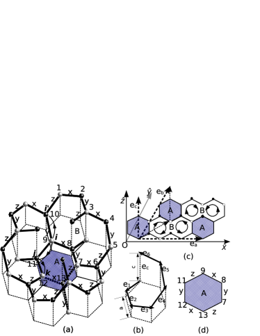
Figure 1: (a) The honeycomb helix lattice. (b) A helix spin chain. (c) The projection to $X-Y$ plane. There are two types of elementary plaquettes, plaquette A and plaquette B . Plaquette $A$ is the shadowed hexagon. Plaquette B covers an area of double hexagon, the oriented circles in the blank double hexagon denote the helix chains with different chirality. (d) The bonding configuration of the hexagon plaquette.

The paper is organized as follows: in section II, we constructed exactly solvable three dimensional spin models on helix-decorated lattice. Their ground states are invariant under time reversal transformation. A topological phase transition from gapless phase to gapped phase is observed. In section III, we established three dimensional chiral spin liquids by doping spins in the helix lattice. Their exact ground states break the time reversal symmetry. In section IV, the topological correlation among loops is studied from the point of view of topological quantum field theory and Jones polynomial. In section V, non-abelian Berry phase of loops is presented. We studied the quantum algebra of loop statistics.

II Exact spin liquid on three dimensional helix lattice

We study the exactly soluble spin models. The exact ground state is short-range spin liquid. They all contain helix structure, so we classify them by the typical helix spin chain embedded in the three dimensional lattice.

II.1 The Honeycomb Helix lattice model

The first spin liquid model we proposed is established on coupled hexagonal helix lattice whose projection to the $X-Y$ plane is Kitaev model on two dimensional Honeycomb lattice(Fig. 1). Two neighboring hexagonal helices have opposite chirality, three pairs of helix string surround one hexagon plaquette. The translational invariant Hamiltonian reads

$$H_{h} = -\sum_{\textbf{i}}\{J_{z}\sigma^{z}_{\textbf{i}}\sigma^{z}_{\textbf{i}-\textbf{e}_{4}}+J_{y}\sigma^{y}_{\textbf{i}}\sigma^{y}_{\textbf{i}+\textbf{e}_{5}}+J_{x}\sigma^{x}_{\textbf{i}}\sigma^{x}_{\textbf{i}-\textbf{e}_{6}}$$ (1)

$$+ J_{y}\sigma^{y}_{\textbf{i}-\textbf{e}_{6}}\sigma^{y}_{\textbf{i}-\textbf{e}_{6}+\textbf{e}_{2}}+J_{x}\sigma^{x}_{\textbf{i}-\textbf{e}_{6}+\textbf{e}_{2}}\sigma^{x}_{\textbf{i}-\textbf{e}_{6}+\textbf{e}_{2}+\textbf{e}_{3}}$$

$$+ J_{z}\sigma^{z}_{\textbf{i}-\textbf{e}_{6}+\textbf{e}_{2}-\textbf{e}_{4}}\sigma^{z}_{\textbf{i}-\textbf{e}_{6}+\textbf{e}_{2}}$$

$$+ J_{y}\sigma^{y}_{\textbf{i}-\textbf{e}_{6}+2\textbf{e}_{2}+\textbf{e}_{3}}\sigma^{y}_{\textbf{i}-\textbf{e}_{6}+\textbf{e}_{2}+\textbf{e}_{3}}$$

$$+ J_{z}\sigma^{z}_{\textbf{i}-\textbf{e}_{6}+2\textbf{e}_{2}+\textbf{e}_{3}+\textbf{e}_{1}}\sigma^{z}_{\textbf{i}-\textbf{e}_{6}+\textbf{e}_{2}+\textbf{e}_{3}}$$

$$+ J_{x}\sigma^{x}_{\textbf{i}-2\textbf{e}_{6}+2\textbf{e}_{2}+\textbf{e}_{3}}\sigma^{x}_{\textbf{i}-\textbf{e}_{6}+2\textbf{e}_{2}+\textbf{e}_{3}}\},$$

where the sum runs over $\textbf{i}=m\textbf{e}_{a}+n\textbf{e}_{b}+l\textbf{e}_{c}$ with basis vector $\textbf{e}_{a}=(3\sqrt{3}a,0,0)$, $\textbf{e}_{b}=(\frac{3\sqrt{3}}{2}a,\frac{3}{2}a,\frac{1}{3}c)$ and $\textbf{e}_{c}=(0,0,c)$(Fig. 1).($a$ and $c$ are two different lattice spacings.) The Hamiltonian describes three dimensional coupled hexagonal helix chains. Each one chiral hexagonal chain is equivalent to an exactly soluble one dimensional alternative coupling spin chain

$$H_{c}=\sum_{{2j}}J_{x}\sigma^{x}_{2j}\sigma^{x}_{2j+1}+J_{y}\sigma^{y}_{2j+1}\sigma^{y}_{2j+2}+J_{z}\sigma^{z}_{2j+2}\sigma^{z}_{2j+3}.$$ (2)

The chirality of helix chain embeds in the operator product of the three component of spin. The chiral operator $\sigma^{z}\sigma^{y}\sigma^{x}$ marks the right-hand helix and $\sigma^{z}\sigma^{x}\sigma^{y}$ characterize the left hand helix(Fig. 1). Usually the non-vanishing chiral order parameter for spin liquid state is defined as

$$\hat{O}_{ijk}=\sum{\vec{\sigma}_{\textbf{i}}\cdot(\vec{\sigma}_{\textbf{j}}\times\vec{\sigma}_{\textbf{k}})}.$$ (3)

Another representation of the chiral operator in terms of the conventional spin-1/2 fermionswen-wilczek-zee is

$$\hat{O}_{ijk}=t_{ij}t_{jk}t_{ki}-t_{ik}t_{kj}t_{ji},$$ (4)

where $t_{ij}\equiv{c^{{\dagger}}_{i,s}c_{j,s}}$ as the hopping operator between two lattice sites. The chirality of helix chain may be characterized by the eigenvalues of $\hat{O}_{ijk}$, $\hat{O}_{ijk}|\psi\rangle=\pm 1|\psi\rangle$.

The Hamiltonian commutes with two elementary loop variables. For loop A in Fig. 1(d), the conserved loop variable $P_{A}$ is given by

$$\hat{P}_{A}=\sigma^{x}_{7}\sigma^{y}_{8}\sigma^{z}_{9}\sigma^{x}_{11}\sigma^{y}_{12}\sigma^{z}_{13}.$$ (5)

And the conserved loop variable $P_{B}$ in loop B (Fig 1(a)) is given by

$$\hat{P}_{B}=\sigma^{y}_{1}\sigma^{z}_{2}\sigma^{z}_{3}\sigma^{z}_{4}\sigma^{x}_{5}\sigma^{y}_{6}\sigma^{z}_{7}\sigma^{z}_{8}\sigma^{z}_{9}\sigma^{x}_{10},$$ (6)

which is equivalent to the product of two hexagon plaquettes with their sharing bonds popping out as inter-layer bonding (Fig. 1 (a)). The eigen values of them are $P_{A}=\pm 1$ and $P_{B}=\pm 1$ because $\hat{P}^{2}_{A}=\hat{P}_{B}^{2}=1$. Notice that $\hat{P}_{A}$ and $\hat{P}_{B}$ may be simultaneously diagonalized because of $[\hat{P}_{A},\hat{P}_{B}]=0$.

According to these conserved loop variables, we may obtain the exact ground state of this model by using Majorana fermions to express spins kitaev ,

$$\sigma^{x}_{\textbf{i}}=ib_{\textbf{i}}^{x}c_{\textbf{i}},\;\;\sigma^{y}_{\textbf{i}}=ib^{y}_{\textbf{i}}c_{\textbf{i}},\;\;\sigma^{z}_{\textbf{i}}=ib_{\textbf{i}}^{z}c_{\textbf{i}}$$ (7)

with constraint $b_{x}b_{y}b_{z}c=1$. Majorana fermions $b_{i}^{x},b_{i}^{y},b_{i}^{z},c_{i}$ obey the anti-commutations relation

$$\{b_{i}^{\alpha},b_{j}^{\beta}\}=2\delta_{\alpha\beta}\delta_{ij},\;\;c_{i}^{2}=1,\;\;\{b_{i}^{\alpha},c_{j}\}=0.$$ (8)

The nearest neighbor spin coupling term reads $\sigma_{i}^{\alpha}\sigma_{j}^{\alpha}=b_{i}^{\alpha}b_{j}^{\alpha}c_{i}c_{j}$, One may verify that the operator $u^{\alpha}_{ij}=ib_{i}^{\alpha}b_{j}^{\alpha}$ commutes with the Hamiltonian and other $u^{\beta}_{ij}$ operators, i.e.,

$$[u^{\alpha}_{ij},H_{d}]=0,\;\;[u^{\alpha}_{ij},u^{\beta}_{kl}]=0.$$ (9)

Therefore, $u^{\alpha}_{ij}$ may be viewed as the bond operator connecting two nearest neighboring lattice sites and they may be though as ’good quantum numbers’ which reflect the real physical conserved loop variables $P_{A}$ and $P_{B}$. To see this point, we define the Wilson loop by a series of product of $u_{ij}$ along a closed path. There are two classes of elementary loops that can not be decomposed into smaller ones in this model, which are exactly the loop A and loop B in Fig. 1. The products of $u_{ij}$ along these loops are no more than the expressions of $\hat{P}_{A}$ and $\hat{P}_{B}$ in Majorana ferioms. Following Lieb’s theoremlieb , the ground state must be vortex free state. The eigenvalue of the hexagon plaquette operator $\hat{P}_{A}$ at vortex free state is ${P}_{A}=1$. This plaquette operator may be interpreted as the magnetic flux through the plaquette, so does the double hexagon plaquette operator $\hat{P}_{B}$. The magnetic field line is perpendicular to the minimal surface of the Wilson loop. We may introduce magnetic helicity to characterize the quantum entanglement between loops of different size.

The Wilson loop operators are good quantum numbers. They share the same Hilbert space with Hamiltonian. Small loops do not gain extra energy when they expand into larger configuration. So these loops have no stress tension. They have the same ground state energy. Any spin configuration along a closed path which preserves $W_{c}=-1$ for Wilson loop defines an elementary excitation. The excited state space is also highly degenerate. There are two types of fundamental quasiparticles in honeycomb helix lattice model, $P_{A}=-1$ and $P_{B}=-1$. The honeycomb helix lattice model has nontrivial loop quasiparticles which obey exotic statistics in three dimensions. Two loops confined in two dimensions could not entangle each other without cutting them up. But in three dimensions, they can avoid crossing each other when they wind around each other by keeping their topology. If they are linked with each other, the continuous transformation between different loop configurations corresponds to the transition between different eigenstates. Quantum entanglement in the degenerate Hilbert space is the origin of non-abelian statistics.

The the vortex free ground state is given by $u_{ij}=+1$. The Hamiltonian becomes quadratic $H_{h}=\sum{h}_{i\mu,j\nu}c_{i,\mu}c_{j,\nu},$ where $i,j$ are the site index of unit cell, $\mu,\nu$ indicates the internal degrees inside the unit cell. In the honeycomb helix model, the unit cell is a bounded pair of plaquette $A$ and plaquette $B$(Fig. 1). The fundamental translational invariant vector of the unite cell is $\textbf{r}_{i}=m\textbf{e}_{a}+n\textbf{e}_{b}+l\textbf{e}_{c}$ with basis vector $\textbf{e}_{a}=(3\sqrt{3}a,0,0)$, $\textbf{e}_{b}=(\frac{3\sqrt{3}}{2}a,\frac{3}{2}a,\frac{1}{3}c)$ and $\textbf{e}_{c}=(0,0,c)$(Fig. 1). Performing the Fourier transformations,

$$h_{\mu\nu}(\textbf{q})=\sum_{j}{e}^{i(\textbf{q},\textbf{r}_{j})}h_{0\mu,j\nu},\;\;c_{\textbf{q},\mu}=\frac{1}{\sqrt{N}}\sum_{j}e^{-i(\textbf{q},\textbf{r}_{j})}c_{j\mu},$$ (10)

we can derive the momentum representation of the Hamiltonian. The exact spectrum is

$$E_{g}(J_{x},J_{y},J_{z},\textbf{{q}})=(J_{x}^{6}-2\cos{3\sqrt{3}aq_{x}}J_{x}^{3}J_{y}^{3}+J_{y}^{6}$$

$$+2\cos({\frac{3}{2}\sqrt{3}}aq_{x}+\frac{3aq_{y}}{2}-\frac{2}{3}cq_{z})J_{x}^{4}{J}_{y}J_{z}$$

$$+4\cos(\frac{3}{2}\sqrt{3}aq_{x}+\frac{3}{2}aq_{y}+\frac{c}{3}q_{z})J^{4}_{x}{J}_{y}J_{z}$$

$$-4\cos(\frac{3}{2}\sqrt{3}aq_{x}-\frac{3aq_{y}}{2}-\frac{cq_{z}}{3})J_{x}{J}_{y}^{4}J_{z}$$

$$-2\cos(\frac{3}{2}\sqrt{3}aq_{x}-\frac{3aq_{y}}{2}+\frac{2cq_{z}}{3})J_{x}J_{y}^{4}J_{z}+5J_{x}^{2}J_{y}^{2}J_{z}^{2}$$

$$+4\cos(cq_{z})J_{x}^{2}J_{y}^{2}J_{z}^{2}+2\cos(\frac{3}{2}\sqrt{3}aq_{x}-\frac{9aq_{y}}{2})J_{x}^{3}J_{z}^{3}$$

$$-2\cos(\frac{3}{2}\sqrt{3}aq_{x}-\frac{9aq_{y}}{2})J_{y}^{3}J_{z}^{3}$$

$$+4\cos(3aq_{y}-(cq_{z})/3)J_{x}J_{y}J_{z}^{4}$$

$$+2\cos(3aq_{y}+\frac{2cq_{z}}{3})J_{x}J_{y}J_{z}^{4}+J_{z}^{6})^{\frac{1}{6}}.$$ (11)

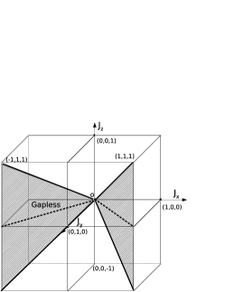
Figure 2: The phase diagram of the honeycomb helix lattice model. The shaded region is the gapless phase.

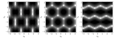
Figure 3: A cross section of the energy spectrum in $q_{x}-q_{y}$ plane. The left panel is in gapless phase, the fermions fill in the low energy region while high energy region is cycled by low energy states. This means there exists closed Fermi surface. The middle panel is the critical region, the Fermi surface is nearly opened. The right panel is in gapped phase. The Fermi surface is completely opened. The dark area is the low energy region which is filled by fermions. The bright area indicates the higher energy region.

The ground state is highly degenerate due to innumerable loop operators which are integral of motion. The whole Hilbert space are divided into two regimes—the gapped phase and gapless phase. The gapless phase falls in the diagram covered by the inequalities:

$$|J_{i}|^{3} \leq 3|J_{i}J_{j}J_{k}|+|J_{j}|^{3}+|J_{k}|^{3},$$

$$3|J_{x}J_{y}J_{z}| \leq |J_{x}|^{3}+|J_{y}|^{3}+|J_{z}|^{3},$$ (12)

where $(i,j,k=x,y,z;\;i\neq{j}\neq{k})$. The gapless phase region in the phase diagram is an infinite triangular area in the plane of $|x|=|y|$(Fig. 2).

The quadratic Hamiltonian expressed by Majorana fermions operator has an equivalent representation in terms of complex fermion operators. We first express the spins by Majorana operators $\sigma^{\alpha}_{\textbf{i}}=ib_{\textbf{i}}^{\alpha}c_{\textbf{i}}$, and then introduce the complex fermionchen on the $\sigma^{z}_{i}\sigma^{z}_{j}$ coupling bonds,

$$d_{r}=(c_{i}+ic_{j})/2,\;\;d_{r}^{\dagger}=(c_{i}-ic_{j})/2.$$ (13)

The spin-spin coupling terms in Hamiltonian can be transformed into standard fermion representation,

$$\sigma^{z}_{i}\sigma^{z}_{j}=u^{z}_{ij}(2d_{\textbf{r}}^{\dagger}{d}_{\textbf{r}}-1),$$

$$\sigma^{x}_{i}\sigma^{x}_{j}=u^{x}_{ij}(d_{\textbf{r}}^{{\dagger}}+d_{\textbf{r}})(d_{\textbf{r}-{\textbf{e}}_{x}}^{{\dagger}}-d_{\textbf{r}-{\textbf{e}}_{x}})$$

$$\sigma^{y}_{i}\sigma^{y}_{j}=u^{y}_{ij}(d_{\textbf{r}}^{{\dagger}}+d_{\textbf{r}})(d_{\textbf{r}-{\textbf{e}}_{y}}^{{\dagger}}-d_{\textbf{r}-{\textbf{e}}_{y}})$$ (14)

where r denotes the center of $\sigma^{z}_{i}\sigma^{z}_{j}$ bonds and $u^{\alpha}_{ij}=ib_{i}^{\alpha}b_{j}^{\alpha}$. The Hamiltonian (1) in the vortex free configuration is transformed into quadratic Hamiltonian expressed by standard fermions. The Fermi surface may be figured out from (11) and has different topological behavior in gapped phase and gapless phase. We plot a cross section of the Fermi surface in Fig. 3. The center of the dark disc area is the lowest energy point. The bright area is the high energy region. The Fermi surface in the left panel of Fig. (3) is periodically arranged bubbles in three dimensional momentum space. Their cross section at $q_{x}-q_{y}$ plane are closed circles without intersection. The Fermi surface in the gapless phase are topologically equivalent to compact sphere in momentum space. The middle panel is critical phase, at which the closed Fermi surface began touching each other but not connected. The right panel of Fig. 3 is in the gapped phase, the closed Fermi surface of gapless phase opened and connected each other(Fig. 3).

The most natural topological index to distinguish the two phases is Hopf index which defines a map of from $S^{3}$ in momentum space to a sphere $S^{2}$ in coherent function space. The nontrivial two dimensional compact manifold embedded in the three dimensional momentum space comes from the gapless solution manifold $E(p)=0$. The Hopf index is an integer which counts how many time the sphere in momentum space wraps the target sphere following the map $f_{Hopf}:S^{3}(p)\rightarrow{S^{2}}$. The nontrivial Hopf index means that the sphere enclose a monopole in momentum space. In the gapless phase, monopoles are enclosed by fermi sphere. They are at the right center of the dark disc areas in Fig. 3. They have either positive charge or negative. The monopole-anti-monopole pairs are fused into vacuum in the gapped phase, so we can not detect them through the Hopf index. The critical region occurs when the monopole-anti-monopole began touching each other but is not near enough to annihilate.

The topological quantum phase transition from confined monopole phase to deconfined monopole phase leads to the divergence of the second order derivative of the ground state energy on the critical boundary. The divergence behavior of approaching the critical point from the gapped phase is totally different from that of gapless phase(Fig. 4). In the gapped phase, a sharp peak far from the critical point is observed in the region of $J_{z}>0$. This peak is finite, it indicates a crossover transition.

Figure 4: The second order derivative of the ground state spectrum at $J_{x}=J_{y}=1$. In the region $-1<J_{z}<1$ is gapless phase and outside is gapped phase.

Now we turn to the spin correlations in the honeycomb helix lattice model. As shown in Ref. baskaran on Kitaev model of two dimensional honeycomb lattice, the two-spin correlation vanishes beyond nearest neighbor separation in different bonding directions. In the three dimensional honeycomb helix lattice model, the two-spin correlation demonstrated the same behavior. The representation of spins by Majorana fermions factorized the eigenstates of physical Hilbert space as gauge sector and corresponding matter sector, $|\psi\rangle=|\psi_{Mg}\rangle|\psi_{g}\rangle$ with

$$\hat{u}_{ij}|\psi_{g}\rangle\equiv{b_{\textbf{i}}^{\alpha}b_{\textbf{j}}^{\alpha}}|\psi_{g}\rangle=u|\psi_{g}\rangle.$$ (15)

The spin operator $\sigma^{\alpha}_{i}$ acting on any eigenstate adds a Majorana fermion at site $i$ and one $\pi$ flux each to the plaquettes intersecting with the bond $\langle{ij}\rangle^{\alpha}$. The two-spin correlation function

$$C^{\alpha\beta}_{\textbf{i}\textbf{j}}(t)=\langle\psi_{g}|\langle\psi_{Mg}|\sigma^{\alpha}_{\textbf{i}}(t)\sigma^{\beta}_{\textbf{j}}|\psi_{Mg}\rangle|\psi_{g}\rangle$$ (16)

measures the probability we will detect the added Majorana fermion and flux at lattice site $j$. If Hilbert spaces of the two-spins at ($\textbf{i},\textbf{j}$) have no overlap on the gauge sector, the two-spin correlation is constantly zero. In this three dimensional honeycomb helix model, the two spins at ($\textbf{i},\textbf{j}$) have no overlap in Hilbert space unless they are nearest neighbors. Therefore two-spin correlation vanishes beyond nearest neighboring separation.

The correlation between plaquette excitations is actually multispin correlation. The non-vanishing multispin correlation comes from the operators which are product of an arbitrary number of the terms that appear in the Hamiltonian. We can compute the multispin correlation using the method in Ref. baskaran . Here we first consider the correlation between the two types of elementary plaquette excitations. As shown in Fig. 1, a spin starts from white lattice site i has three different propagating direction. The interlayer spin correlation $C^{\alpha\beta}_{\textbf{i}\textbf{i}^{\prime}}(t)$ are sharply cut off at nearest neighbor separation. This two-spin correlation measures the coupling between two $\hat{P}_{b}$ plaquette excitations. The coupling between $\hat{P}_{a}$ plaquette excitation and $\hat{P}_{b}$ plaquette excitation is measured by three-spin correlation. One spin flip at i excites two plaquette excitations, $\hat{P}_{A}=-1$ and $\hat{P}_{b}=-1$. Their sharing boundary is along $\textbf{i}\rightarrow\textbf{j}\rightarrow\textbf{k}$. For a spin flip propagating along the path $\textbf{i}\rightarrow\textbf{j}\rightarrow\textbf{k}$, the nonzero three-spin correlation

$$C^{\alpha\beta\gamma}_{\textbf{i}\textbf{j}\textbf{k}}(t)=\langle\psi_{g}|\langle\psi_{Mg}|\sigma^{\alpha}_{\textbf{i}}(t)\sigma^{\beta}_{\textbf{j}}(t)\sigma^{\gamma}_{\textbf{k}}(t)|\psi_{Mg}\rangle|\psi_{g}\rangle$$ (17)

ends at another white site k. The two elementary plaquette operators are the smallest loops, they can not be decomposed into smaller ones. As for the more complex loop-loop correlation, we shall introduce non-abelian Chern-Simons theory in the following sections.

We introduce the other three dimensional helix models in the following. They have more or less similar property as the honeycomb helix model. We left the exact solution and present only the spin-spin coupling configuration.

II.2 The Square Helix model

$\begin{array}[]{c@{\hspace{0.01in}}c}\includegraphics[scale={0.35}]{square2.eps}\hfil\hskip 0.72229pt\\ \mbox{\bf(I)}\hfil\hskip 0.72229pt&\mbox{}\\ \includegraphics[scale={0.35}]{square3.eps}\hfil\hskip 0.72229pt\\ \mbox{\bf(II)}\hfil\hskip 0.72229pt&\mbox{}\end{array}$

Figure 5: (I)-(a) The square helix lattice model. (I)-(b) The triangle helix model on Cu-sublattice in ${C{u}}_{6}{S{i}}_{6}{O}_{3}\cdot 6{H_{2}O}$.

(II)-(a) An equivalent demonstration of square helix model on cubic lattice. (II)-(b) The deformed triangle helix model on cubic lattice.

The square helix model is composed of alternative $XY$ spin chains each of which has four nearest neighboring chains coupled to one another through $\sigma^{z}\sigma^{z}$ bonding(Fig. 5, (a)). The Hamiltonian includes two parts, $H_{SH}={\sum}H_{xy}+H_{z}$,

$$H_{SH} = \sum_{{ij,k=even}}[J_{y}\sigma^{y}_{ij,k-1}\sigma^{y}_{ij,k}+J_{x}\sigma^{x}_{ij,k}\sigma^{x}_{ij,k+1}]$$ (18)

$$+ \sum_{i{\pm}n,j,k{\pm}2n}[J_{z}\sigma^{z}_{i-1,j,k}\sigma^{z}_{i,j,k}]$$

$$+ \sum_{i,j{\pm}n,k{\pm}2n}[J_{z}\sigma^{z}_{i,j,k+1}\sigma^{z}_{i,j+1,k+1}].$$

A single helix chain is exactly the same single $XY$ spin chain in two dimensional Kitaev model, which is equivalent to one dimensional Ising model with transverse fieldfeng . The multispin correlation function along a single helix chain demonstrates a long range order,

$$S^{xx}_{2j}=\lim_{j\rightarrow\infty}\langle\prod^{2j}_{k=1}\sigma^{x}_{k}\rangle\sim[1-(J_{y}/J_{x})^{2}]^{1/4}.$$ (19)

In the three dimensional square-helix model, it is the product operator of the bonding terms in Hamiltonian that has nonzero multispin correlation. While two-spin correlation in real lattice space vanishes at the nearest neighboring separationbaskaran . The chiral operator is the combination of different product of three spin operators, it is a good quantity to characterize the quantum entanglement of three spins.

The Hamiltonian (18) is exactly soluble following a similar procedure as that in honeycomb helix model except a different gauge fixing. There are two types of fundamental plaquettes in square helix model. It is more clear to see the picture by deforming the square helix lattice into cubic lattice(Fig. 5). The energy minimum of ground state is achieved by $0-\pi-0-\pi\cdots$ alternative flux pattern following Lieb’s theorem. The integrals of motion $P_{A}$ take a phase $2\pi$ for all irreducible plaquette A, $\hat{P}_{A}=\sigma^{z}_{1}\sigma^{z}_{2}\sigma^{z}_{3}\sigma^{x}_{4}\sigma^{y}_{5}\sigma^{z}_{6}\sigma^{z}_{7}\sigma^{z}_{8}\sigma^{x}_{9}\sigma^{y}_{10}=e^{i2\pi}$, and for all plaquette B, $\hat{P}_{B}=\sigma^{y}_{1}\sigma^{y}_{2}\sigma^{x}_{3}\sigma^{x}_{4}\sigma^{y}_{5}\sigma^{y}_{6}\sigma^{x}_{7}\sigma^{x}_{8}=e^{i\pi}$.

Elementary plaquette excitations are produced by flipping odd number of spins along the plaquettes A and B. At the excited states, the phase pattern of the two palquettes are $P_{A}=-1$ and $P_{B}=+1$. The highly degenerate eigenstates are classified by different spin configurations. The spin flip at lattice site i excites four $\pi$ flux each in its four neighboring plaquettes. Four plaquette excitations are always generated and annihilated at the same time. So there are many degree of freedom to operate on them. Two of the four plaquette excitations may share a strong four-spin correlation in $k$-direction,

$$C^{yzxx}_{k,k+1,k+2,k+3}=\langle\sigma^{y}_{ij,k}\sigma^{z}_{ij,k+1}\sigma^{x}_{ij,k+2}\sigma^{x}_{ij,k+3}\rangle.$$ (20)

This four-spin correlation only covers four neighboring lattice sites,

$$C^{yzx\lambda}_{k,k+1,k+2,k+m}(t)=0,m>3.$$ (21)

While another two of the four plaquette excitation are connected only by nonzero two-spin correlation. Thus the correlation between plaquette excitations is different along different direction.

II.3 The triangle helix model on Dioptast Lattice

The triangle helix model is established on a three dimensional lattice which exist in nature. The $Cu$ atoms in dioptase ${C{u}}_{6}{S{i}}_{6}{O}_{3}\cdot 6{H_{2}O}$ construct the exact triangle helix lattice, $Cu$-atoms form chiral chains along $z$-axes and project a honeycomb configuration to the $X-Y$ planegros .

The exact solution of the Heisenberg spin-spin coupling hamiltonian on the dioptase lattice is hardly reachable. We derived an exactly soluble model by introducing Kitaev-type spin-spin coupling interactions along different bonds on this three dimensional lattice(Fig. 2(b)). The projection of the triangle helix model to $X-Y$ plane is a two dimensional chiral spin liquid model constructed in Refs. yao yangsun which has a stable ground state spontaneously breaking time reversal symmetry. While our three dimensional triangle helix model is invariant under time reversal transformation. The two elementary plaquettes, octagon $\hat{P}_{8}$ and dodecagon $\hat{P}_{12}=\sigma^{x}_{1}\sigma^{z}_{2}\sigma^{y}_{3}\sigma^{x}_{4}\sigma^{z}_{5}\sigma^{y}_{6}\sigma^{x}_{7}\sigma^{z}_{8}\sigma^{y}_{9}\sigma^{x}_{10}\sigma^{z}_{11}\sigma^{y}_{12}$, are both in $\pi-$flux phase at ground states. Unlike the quantum phase transition from anti-ferro-magnetically ordered state to a quantum spin liquid in magnetic crystal ${C{u}}_{6}{S{i}}_{6}{O}_{3}\cdot 6{H_{2}O}$, the quantum phase transition here in the triangle helix model is between two topologically distinguished spin liquid states.

II.4 The Square-Hexagon-Helix Lattice Model

The square-hexagon-helix lattice model projects one of the two dimensional modelsyangsun with Kitaev type’s coupling in $X-Y$ plane. The hexagon helix with opposite chirality are separated by isolated squares. The spatial distribution of the helixes is a pillar array on Kagome lattice(Fig. 6). Further observation shows, the square-hexagon-helix model is composed of three coupled Ising models which are established on multilayer Kagome lattice.

$\begin{array}[]{c@{\hspace{0.01in}}c}\lx@intercol\mbox{}\hfil\lx@intercol&\lx@intercol\mbox{}\hfil\lx@intercol\\ \includegraphics[scale={0.25}]{tricomb.eps}\hfil\hskip 0.72229pt&\includegraphics[scale={0.2}]{tricomb-cell.eps}\\ \mbox{\bf(a)}\hfil\hskip 0.72229pt&\mbox{\bf(b)}\end{array}$

Figure 6: (a) The square-hexagon-helix Lattice model. (b) An equivalent configuration of square-hexagon-helix Lattice model on multi-layers Kagome lattice.

III Three dimensional chiral spin liquid models

In the sections above, we have derived four typical spin models which are exactly soluble in three dimensions. Their ground states with short range interaction are spin liquid states. It has been a long history to look for three dimensional chiral spin liquid, so far there is still no exact soluble three dimensional model to confirm its existence. In this section, we shall construct a series of three dimensional chiral spin liquid models. They are exactly solvable. Their exact stable ground states spontaneously break the time reversal symmetry. These chiral spin liquids are likely to be realized by ultracold atoms trapped in cubic optical lattice.

III.1 Chiral Square Helix Model

We add two spins at all of the horizontal $\sigma^{z}\sigma^{z}$ bonds in the cubic version of deformed square helix lattice(Fig. 5 (II)-(a)). One is at $1/3$ of one lattice spacing and the other is at $2/3$. We shift the added spins vertically a half lattice spacing along $z$-axis. If the spins are assumed to have only the nearest neighboring interaction, we get the first chiral spin liquid in three dimensions(Fig. 7 (a)). The Hamiltonian of the chiral square helix reads

$$H_{cc} = -\sum_{{ij,k=even}}[J_{y}\sigma^{y}_{ij,k-\frac{3}{4}}\sigma^{y}_{ij,k-\frac{1}{4}}+J_{z}\sigma^{z}_{ij,k-\frac{1}{4}}\sigma^{z}_{ij,k+\frac{1}{4}}$$

$$+ J_{x}\sigma^{x}_{ij,k+\frac{1}{4}}\sigma^{x}_{ij,k+\frac{3}{4}}+J_{z}\sigma^{z}_{ij,k+1-\frac{1}{4}}\sigma^{z}_{ij,k+1+\frac{1}{4}}]$$

$$+ \sum_{i{\pm}n,j,k{\pm}2n}[J_{y}\sigma^{y}_{i-\frac{1}{3},j,k}\sigma^{y}_{ij,k+\frac{1}{4}}+J_{x}\sigma^{x}_{i-\frac{1}{3},j,k}\sigma^{x}_{ij,k-\frac{1}{4}}$$

$$+ J_{z}\sigma^{z}_{i-\frac{2}{3},j,k}\sigma^{z}_{i-\frac{1}{3},j,k}$$

$$+ J_{y}\sigma^{y}_{i-1,j,k+\frac{1}{4}}\sigma^{y}_{i-\frac{2}{3},j,k}+J_{x}\sigma^{x}_{i-1,j,k-\frac{1}{4}}\sigma^{x}_{i-\frac{2}{3},j,k}]$$

$$+ \sum_{i,j{\pm}n,k{\pm}2n}[J_{y}\sigma^{y}_{i,j,k+\frac{3}{4}}\sigma^{y}_{i,j+\frac{1}{3},k+1}$$

$$+ J_{x}\sigma^{x}_{i,j,k+1+\frac{1}{4}}\sigma^{x}_{i,j+\frac{1}{3},k+1}$$

$$+ J_{z}\sigma^{z}_{i,j+\frac{1}{3},k+1}\sigma^{z}_{i,j+\frac{2}{3},k+1}$$

$$+ J_{y}\sigma^{y}_{i,j+\frac{2}{3},k+1}\sigma^{y}_{i,j+1,k+\frac{3}{4}}+J_{x}\sigma^{x}_{i,j+\frac{2}{3},k+1}\sigma^{x}_{i,j+1,k+\frac{5}{4}}].$$

Our interest focus mainly on the gauge symmetry of exact ground state. As shown in Fig. 7 (a), there are three elementary plaquettes: a triangle and two polygons. One of the two polygons has sixteen bonds, the other covers twenty bonds. The energy is minimized by uniform flux configuration. The elementary plaquettes are all in $\pi$-flux phase at ground state. The $\pi-$flux of triangular plaquette flips under time reversal transformation. Although the two polygon plaquettes are invariant under time reversal transformation, the global flux pattern spontaneously breaks the time reversal symmetry. Thus the ground state is highly degenerate chiral spin liquid.

The fractionalized elementary excitations are loop excitations in the three dimensional chiral spin liquid. Large loop operator is the product of the elementary plaquettes covered by its minimal surface. If the loop has odd number of links, there must be odd number of triangular plaquettes confined in the area surrounded by the loop. A spin flip adds $\pi$-flux each to the plaquettes intersecting at that point. To some extend, the time reversal transformation behaves like transition operator between excited states and ground states. The loop with odd number of particles spontaneously breaks the time reversal symmetry.

The correlation between plaquette excitations is measured by multispin correlation which are spatially anisotropic. For example, a spin flip at site q excites four plaquettes vertices sharing a bond along $z$-axis. Two of them share a strong six-spin correlation

$$C_{\textbf{q}\textbf{q}_{1}\textbf{q}_{2}\textbf{q}_{3}\textbf{q}_{4}\textbf{p}}^{\alpha\beta\gamma\lambda\eta\kappa}=\langle\sigma^{\alpha}_{\textbf{q}}\sigma^{\beta}_{\textbf{q}_{1}}\sigma^{\gamma}_{\textbf{q}_{2}}\sigma^{\lambda}_{\textbf{q}_{3}}\sigma^{\eta}_{\textbf{q}_{4}}\sigma^{\kappa}_{\textbf{p}}\rangle.$$ (23)

While another pair of plaquette excitations are only connected by two-spin correlation which are sharply cut off beyond nearest neighbors. This suggest that the fusion rules for plaquette excitations in this mode might be more complex than that in two dimensions.

$\begin{array}[]{c@{\hspace{0.01in}}c}\lx@intercol\mbox{}\hfil\lx@intercol&\lx@intercol\mbox{}\hfil\lx@intercol\\ \includegraphics[scale={0.25}]{square6.eps}\hfil\hskip 0.72229pt&\includegraphics[scale={0.25}]{kagome.eps}\\ \mbox{\bf(a)}\hfil\hskip 0.72229pt&\mbox{\bf(b)}\end{array}$

Figure 7: (a) The chiral square helix model on cubic lattice. (b) The chiral dodecagon helix model. The character structure is the dodecagonal helix.

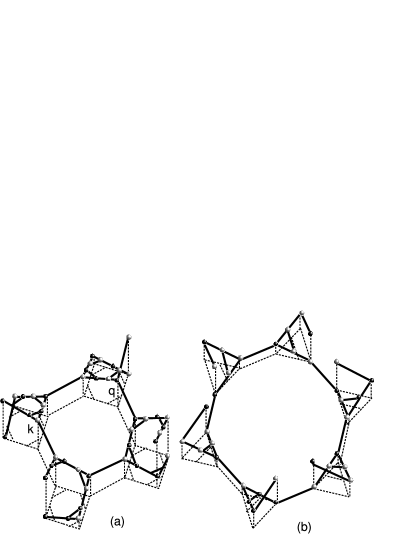
Figure 8: (a) The chiral square helix model on the original square helix lattice. (b) The chiral spin liquid model on the triangular decorated dioptast lattice.

III.2 The general principal to construct other artificial chiral spin liquid model

There are many other ways to construct three dimensional chiral spin models with Kitaev’s type of coupling, which requires that each lattice site branches out only three different bonds corresponding to $\sigma_{x}\sigma_{x}$, $\sigma_{y}\sigma_{y}$ and $\sigma_{z}\sigma_{z}$. For example, we add two spins at every bond to divide it into three equal sections, and assume spins only interact with nearest neighbors, it naturally leads to a chiral spin liquid in three dimension. In Fig. 8, we present two examples, the triangular decorated square helix model and triangle helix model. If one deforms the triangular decorated square helix lattice model(Fig. 8 (a)) into cubic lattice, the triangular decorated square helix is exactly the chiral square helix model. One can also construct other models by dividing some selected bonds into $n(n=2,3,4...)$ identical pieces and adding spins on the adjoint points with properly arranged bonding direction. The triangular decorated triangle-helix model(Fig. 8 (b)) is one of such constructions, to construct this model, we add one spin each on the two bonds branched from the same lattice site.

Another different way of constructing is to spiral polygon plaquettes up. For example, we construct the dodecagon helix lattice model which has the same two dimensional projection to $X-Y$ plane as the diopaste lattice. Here it is the dodecagon that spirals up with triangles as bridge between dodecagonal helixes(Fig. 7). We can also obtain this chiral spin liquid model by replacing each lattice site in the honeycomb helix model(Fig. 1) with a triangle. If we keep replacing the lattice sites with triangles time and time again, it finally leads to the fractal lattice model. This fractal model is different from Bethe lattice. There is no closed loop in Bethe lattice, but in this fractal lattice model, it is all sorts of loops that construct the whole lattice. These loops form the complete set of integrals of motion. Scale invariance lays in the heart of these exactly soluble fractal lattice models.

Now we see that three dimensional chiral spin liquid emerges following a rather simple doping construction. The only thing we need is local interaction between nearest neighboring spins. When it comes to existing material in nature, it is possible get chiral spin liquid by doping spins in conventional three dimensional lattice.

IV Topological Correlation of entangled loops in three dimensional chiral spin liquid

In the exactly soluble spin models obtained above, a closed path $C$ consists of a series of bonds. Defining $\hat{h}^{\gamma}_{ij}=\sigma^{\gamma}_{i}\sigma^{\gamma}_{j}$ for a given bond $\gamma$, the product of $\hat{h}^{\gamma}_{ij}$ along $C$ is a $Z_{2}$ gauge invariant quantity which is nothing but the Wilson loop $W_{C}=\prod_{\gamma\in C}\hat{h}^{\gamma}_{ij}$. The Hilbert space is divided into many gauge equivalent class $\{|\psi_{C}\rangle\}$ corresponding to $W_{C}$ with

$$W_{C}|\psi_{C}\rangle=\pm|\psi_{C}\rangle.$$ (24)

Quantum information is encoded in this Hilbert space. The gauge invariant stats can only be distinguished by global operation, which protects the quantum information from decoherence due to local quantum entanglement with environment.

Non-abelian excitations in three dimensional chiral spin liquid serve as elementary qubits to perform quantum computation. Basic logic gate may be constructed by designed braiding operation. To perform topological quantum computation, we shall operate on excitations obeying non-abelian braiding statistics. Point quasiparticles in three dimensions are either fermion or boson and thus they are not good candidates. It is the loop excitations that satisfy non-commutable relation during the unitary evolution in ground state subspace.

We first consider the unknotted loops which are not entangled or linked with each other. If the loop correlation is extended to strong and weak coupling limit of lattice gauge theory, it shows that the loop correlations $S_{\alpha\beta}:=\langle{W_{C_{\alpha}}W_{C_{\beta}}}\rangle$ decay exponentially with distance. At high temperature, the decay width is governed by the area $A$ encapsulated by the two loops, $S_{\alpha\beta}\propto{e^{cA}}$. At low temperature, the total perimeter $|C_{\alpha}|+|C_{\beta}|$ determines the decay behavior, $S_{\alpha\beta}\propto{e^{c(|C_{\alpha}|+|C_{\beta}|)}}$.

Loop-loop correlation is actually bipartite multi-spin correlation which can be calculated using the method developed in Ref. baskaran . The area $\hat{A}_{\alpha}$ enclosed by loop $C_{\alpha}$ is composed of a collection of elementary plaquettes. The Wilson loop is just the product of all the elementary plaquette operators

$$W_{C_{\alpha}}=\prod_{i}{\hat{P}_{i}^{a}},$$ (25)

$a$ indicates the type of elementary plaquette. For example, $a=1,2,3$ in the chiral square helix model, $C_{1}$ and $C_{2}$ represent the two polygons and $C_{3}$ represents the triangular plaquette. The degenerate Hilbert space of loop is the direct product of the subspace of all the elementary plaquettes in $\hat{A}_{\alpha}$. For a given loop $C_{\alpha}$, there exist many different $\hat{A}_{\alpha}$ such that $\partial\hat{A}_{\alpha}=C_{\alpha}$. The dominate contribution to the correlation of two loops comes from the minimal surface $M$ encapsulated between them. The boundary of the minimal surface is just the two loops, $\partial{M}=C_{\alpha}+C_{\beta}$. We denote its Hilbert space as $\Psi_{M}$, the two loop correlation reads

$$S_{\alpha\beta}(t)=\langle\Psi_{\beta}|e^{i(H-E)t}\hat{W}_{C_{\alpha}}(t)\hat{W}_{C_{\beta}}\rangle|\Psi_{\alpha}\rangle,$$ (26)

which has an explicit expression

$$S_{\alpha\beta}(t)=\langle\Psi_{g}|e^{i(H-E)t}\prod_{\langle{ij}\rangle_{\alpha}}\sigma^{\gamma}_{{i}}\sigma^{\gamma}_{{j}}\prod_{\langle{kl}\rangle_{\beta}}\sigma^{\eta}_{{k}}\sigma^{\eta}_{{l}}|\Psi_{g}\rangle.$$ (27)

Expressing the spins in terms of Majorana fermions, we may divide the Hilbert space into different gauge sectors according to the static $Z_{2}$ gauge field operators $u_{ij}\equiv i{b_{\textbf{i}}^{\gamma}b_{\textbf{j}}^{\gamma}}$. The multispin correlation can be computed on the gauge sectorsbaskaran . However this computation is hard to tell the physical picture of topological entanglement between loops.

In order to see the topological correlation more clearly, we take a more physical picture in the continuum limit. We view a loop as an electric current source radiating magnetic field. The topological correlation between loops is equivalent to the topological entanglement between magnetic field circles. Obviously no matter how far the loops are separated, the magnetic field lines are always entangled. When it comes to the knotted loops which are linked, entangled one anther, besides the conventional loop correlation which decays as their spatial separation increases, there exist topological correlation which relies on the global topology of links instead of the average distance between them. The topological correlation is immune to local fluctuation in space. Each knotted Wilson loop operator projects a subspace, this topological correlation is a good quantity to measure the quantum entanglement between different sectors of the total Hilbert space.

To study the topological correlation of linked, knotted loops, we first take a preview in the continuum limit. Considering the Hopf link, in which two unknotted rings locked each other up, there is only one crossing point between loop $C_{\alpha}$ and the minimal surface of loop $C_{\beta}=\partial{A}_{\beta}$. The two loops have no intersection. For a more general case, one loop winds around another many times, the winding number is identical to intersecting points

$$C_{\alpha}\cap{{A_{\beta}}}=\{P_{i},i=1,2,...,m\}.$$ (28)

The number of intersecting points is identified with a topological number called Linking number $L_{k}$ which can be calculated by Gauss link integral of lattice gauge potential. The three dimensional Jordan-Wigner transformation mapping spin to fermions defined a gauge transformation,

$$\sigma^{+}_{\textbf{i}}=Uc^{{\dagger}}_{\textbf{i}},\;\;\sigma^{-}_{\textbf{i}}=c_{\textbf{i}}U^{{\dagger}},\;\;\sigma^{z}_{\textbf{i}}=c^{{\dagger}}_{\textbf{i}}c_{\textbf{i}}-\frac{1}{2},$$

$$U=e^{i\sum_{\textbf{j}\neq\textbf{i}}{j^{\alpha}}\omega(\textbf{j}-\textbf{i})}.$$ (29)

The gauge potential is introduced as $A_{\mu}=\nabla_{\mu}\omega.$ The corresponding magnetic fieldbock is

$$B(i,j,k)=\nabla\times{A(i,j,k)}$$ (30)

with discrete derivative

$$\partial_{i}A(i,j,k)=A_{i+1,j,k}-A_{i,j,k}.$$ (31)

The integral of the gauge field along $C_{a\alpha}$ is Wilson loop $W_{C_{\alpha}}$.

The physicists’ approach to the linking number of two loops $C_{\alpha}$ and $C_{\beta}$ is using analogy with Amp$\acute{e}$re’s law. Gauss link integral on the two entangled loops does not depend on the physical meaning of vector field tangent to them, they are valid for any physical vector field. So we think of loop $C_{\alpha}$ as being a wire carrying an electric current I. The line integral of the generated magnetic field $B$ around the closed curve is $4\pi{L_{k}}I$, where $L_{k}$ is the linking number which count how many times the current winds around another closed loop. The linking number is just number of nontrivial intersecting points between $C_{\alpha}$ and the minimal surface of $C_{\beta}$. One may also deduce this directly from the Biot-Savart Law. Therefore we define the topological correlation as

$$\hat{S}^{T}_{\alpha\beta}(t)\;\;\;{\propto}\;\;\;m\;g_{\alpha\beta}\;\;\;{\propto}\;\;\;L_{k}\;g_{\alpha\beta}$$ (32)

with $L_{k}$ as a topological index. A spin flip at the crossing point $P_{i}$ excites the two loops at same time, thus they have overlap in the gauge sectors of Hilbert space. Then we derived a nontrivial contribution to the multispin correlation function of two loops. This topological correlation survives local fluctuation and are valid for thermal states. It should be pointed out here that some intersecting points would disappear during topological transformation. Those points do not contribute to the topological correlation. In the following when we mention intersecting points, it always means the nontrivial intersecting points which can not be eliminated by topological transformation.

Knotted Wilson loops in the three dimensional spin models above also commute with Hamiltonian, they are good quantum numbers. The topological correlation between linked knots can be described by topological quantum field theory. Witten found the quantum field theory to describe a wide class of topological invariant from the non-abelian Chern-Simons theorywitten . For a link containing a collection of knotted, linked loops in three dimensional manifold $L=\{C_{i},i=1,2,3...\}$, we can compute the multiloop correlation function between its component $C_{i}$,

$$Z(L)=\langle{C_{i}{\cdots}C_{i}}\rangle=Z{(M)}^{-1}\int[{\mathcal{D}}A]{e^{iS}}\prod_{i=1}^{k}W_{l}(C_{i}),$$ (33)

where $W_{C}=Tr(Pe^{i\oint{A^{\mu}d\gamma^{\mu}}})$ is the Wilson loop. $S$ is the non-abelian Chern-Simons action $S=\frac{k}{4\pi}\int_{M}Tr(A\wedge{dA}+\frac{2}{3}A\wedge{A}\wedge{A})$, the first term in the non-abelian action represents the local magnetic Helicity

$$H_{elicity}=\epsilon_{ijk}B_{i}\partial_{j}A_{k}.$$ (34)

$Z(L)$ is a gauge invariant which provides us a topological quantity to classify the geometric configuration of linked loops at different eigenstates.

We compact the three dimensional lattice manifold into $S^{3}$ in the continuum limit. A sophisticate link embedded in this $S^{3}$ may be decomposed into two parts by cutting the $S^{3}$ using an $S^{2}$ as section manifold. We choose a proper cutting point so that the left piece $M_{L}$ contains most complicated stuff of the link, and keep the right piece $M_{R}$ as the simplest link configuration. The Feynmann path integral on $M_{L}$ determines a vector $|\chi\rangle$ in the physical Hilbert space, the Feynmann path integral on $M_{R}$ determines a dual vector $|\psi\rangle$. The partition function is the natural paring of the two vectors

$$Z(L_{+})=\langle\chi|\psi\rangle,$$ (35)

$L_{+}$ denote the over crossing of the two loops on the $M_{R}$. The separated two parts of link puncture four points on the cross section manifold. The four punctured points represent two spin fields $\sigma$ and their corresponding antiparticles. Braiding these quasiparticles on $S^{2}$ leads two different configuration manifolds of the link, which we denote as $M_{1}$ and $M_{2}$. The corresponding path integral on $M_{1}$ and $M_{2}$ contributes another two different vectors $|\psi_{1}\rangle$ and $|\psi_{2}\rangle$. The two vectors can be viewed as being generated by applying braid group operations on the original dual vector $|\psi\rangle$ of $M_{R}$. In topological quantum field theory, the Skein relation is encoded in

$${\alpha}\langle\chi|\psi\rangle+\beta\langle\chi|\psi_{1}\rangle+\gamma\langle\chi|\psi_{2}\rangle=0.$$ (36)

Namely,

$${\alpha}Z(L_{+})+{\beta}Z(L_{0})+{\gamma}Z(L_{-})=0.$$ (37)

$L_{0}$ denotes the zero crossing in $M_{1}$ and $L_{-}$ denotes the under crossing in $M_{2}$. Here the three parameters $\{\alpha,\beta,\gamma\}$ depends on the special models. This relation is the fundamental constrain on the multi-loop correlation of sophisticate links in our exact three dimensional spin models.

The topological correlation is invariant no matter how large one loop expands continuously. Any local change that break the topology of a link during evolution would sent out a signal by correlation function. The linking number $L_{k}$ would jump from $m$ to $m\pm{i},(i\neq 0)$, so does the topological correlation function $S^{T}\propto{L_{k}}$. If the loop breaks apart at the crossing lattice site, the topology of link changed, this change would be detected by the topological correlation function.

As one loop expands without cutting the other loop, the eigenstates correspondingly evolute from a state of one loop to another in Hilbert space, but the topological correlation remains invariant. Therefore local perturbation does not destroy the topological signal if the two loops does not intersect. This topological quantum entanglement does not depend on temperature, so it is a very good candidate for quantum memory. Three dimensional materials in natural are very promising for topological quantum computation.

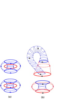
Figure 9: (a) one loop wraps another loop, the chirality of the two loops in the upper is opposite and is same in the lower half-plane. (b)The exchange of two loops. The upper diagram depicts the world sheet of two loops with one loop flips its chirality during the exchange. The lower diagram depicts the case that two loops keep their chirality invariant during the exchange.

V statistics of strings in three dimensions

The statistics of point particles is characterized by the phase change of many body wave function during the exchange of particles, for bosons, $|\psi(x_{1},x_{2})\rangle=e^{i2\pi}|\psi(x_{2},x_{1})\rangle$, and for fermions, $|\psi(x_{1},x_{2})\rangle=e^{i\pi}|\psi(x_{2},x_{1})\rangle$. We are led back to the initial state

$$|\psi(x_{1},x_{2})\rangle=e^{i2\gamma\pi}|\psi(x_{2},x_{1})\rangle.$$ (38)

After performing the exchange twice. The anyon statistics falls in the range of phase $\gamma$ varying continuously from $1/2$ to $1$. In three dimensions, any wrapping path of one particle around another can be topologically contracted to a point, that means two interchange is equivalent to an identical map, so the statistics of point particles is either fermionic or bosonic.

The emergent string excitations bear exotic statistics in three dimensions. For the simplest illustration, if two unentangled and unknotted vortex rings leap through each other, a nontrivial statistical phase may emerge as Berry’s phaseniemi . The leapfrogging vortex rings are a vivid demonstration of loop braid groupbaez for a collection of unknotted, unlinked loops.

When it comes to discrete loops in three dimensional lattice, many exotic phenomena pop out. Any closed loop in the three dimensional exactly solvable models discussed above commute with the corresponding Hamiltonian. The string operator along an oriented path $C_{\alpha}$ reads

$$\hat{O}_{\alpha}=\prod_{i\in{C_{\alpha}^{\circlearrowleft}}}^{n_{\alpha}}\sigma^{\gamma_{i}}_{i},$$ (39)

$\circlearrowleft$ denotes the counterclockwise order of operator product. Its complex conjugate string operator $\hat{O}_{\alpha}^{{\dagger}}=\prod_{i\in{C^{\circlearrowright}_{\alpha}}}^{n_{\alpha}}\sigma^{\gamma_{i}}_{i}$ has a clockwise product order. Since $[\hat{O}_{\alpha},H]=0$, the ground state of loop is an eigenstate of $\hat{O}_{\alpha}$ following the equation

$$\hat{O}_{\alpha}|\psi_{\alpha}\rangle=z|\psi_{\alpha}\rangle,z=\pm 1.$$ (40)

In the degenerate Hilbert space of ground state, an initial state may end up with different final states after adiabatic evolution along a closed path. The conventional Berry phase needs to be generalized to a matrix of inner product between degenerate states. Notice that a loop sweeps out a two dimensional world sheet, the Berry phase $\phi=\langle{\psi(R)}|\nabla_{R}|\psi(R)\rangle$ of point particle along an one dimensional trajectory must be extended to cover the extra dimension of loop $C_{\alpha}(s)$, where $s$ measures the distance along the curve. We start from the general eigenfunction of time-dependent Schr$\ddot{o}$dinger equation, an adiabatic evolution in the degenerate subspace follows

$$|\psi_{\alpha}(C(s))\rangle=e^{-i\int_{0}^{T}E(t)}e^{i\phi_{\alpha\beta}}|{\psi_{\beta}}(C(s))\rangle,$$ (41)

where

$$\phi_{\alpha\beta}=i\int_{0}^{T}dt\int_{T}{{dV}}\langle{\psi_{\alpha}}|{\partial_{t}\psi_{\beta}}\rangle$$ (42)

is the extended Berry phase. We first consider an unknotted, unlinked loop $\emph{C}_{\alpha}$. The minimal surface $\Sigma_{\alpha}(t)$ bounded by $\emph{C}_{\alpha}$ subtends a solid angle $\Omega_{\alpha}(R,t)$ at point $R$. A collection of solid angles of different loops $\{\Omega_{\alpha}(R,t),\Omega_{\beta}(R,t),\cdots\Omega_{\gamma}(R,t)\}$ constitute one geometric representation of loops. In the continuum limit, the gradient of the solid angle field $-\nabla\Omega(R,t)$ induces an effective magnetic field which circulates around the loop. This magnetic field could be computed from the Biot-Savart law. The extended Berry phase in Eq. (42) has explicit expression in terms of solid angle field,

$$\phi_{\alpha\beta}=i\int_{0}^{T}dt\int_{T}{{dV}}\langle{\psi_{\alpha}}|\psi_{\beta}\rangle\partial_{t}\Omega(R,t).$$ (43)

If we assume the probability density $\rho_{\alpha\beta}=\langle{\psi_{\alpha}}|\psi_{\beta}\rangle$ is homogeneous, the quantum mechanical phase is proportional to the volume which is encapsulated by the world sheet bounded by the two loops $\emph{C}_{\alpha}$ and $\emph{C}_{\beta}$.

Exotic statistics phase is strongly dependent on the chirality of loops. For example, consider a red loop and a blue loop with the same orientation(Fig. 9), the exchange of the two loops sweeps out a torus surface, the statistical phase is proportional to the volume of the torus ${V}_{\alpha\beta}^{torus}$. If the chirality of one loop flips during the exchange, the world sheet becomes Klein bottle which is unoriented manifold with only one side. There is no definite volume integral for the quantum mechanical phase in this case. Here we take another equivalent but simpler exchange procedure by wrapping the solid red loop around the dashed blue loop. The dashed blue loop enclosed in the torus surface of world sheet behaves like electric current which produces a magnetic field following the Biot-Savart law

$$dB_{b}=c_{0}r^{-3}d\textbf{s}_{b}\times{{\textbf{r}}}.$$ (44)

The volume integral enclosed by the torus is computed from

$$V={\int}dV={\int}dB_{b}\times{d\textbf{s}_{r}}\cdot{dR}.$$ (45)

If the two loops have the same chirality, the statistical phase factor is proportional to the volume of a torus world sheet, it is positive. On the other hand, if the loops have opposite chirality, the volume integral is negative. Generally speaking, two loops with opposite chirality behave like fermions, while two loops with same chirality obey bosonic statistics.

Another key element governing the statistics of loops is the total number of particles confined along the loop. The vortex excitation in the minimal surface surrounded by the loop behaves like quasiparticles of magnetic flux. We simplify the statistics of two loops as that between two quasi-particles. If the sum of spins of one loop is half integer, the quasiparticle is fermion. If the total spin is integer, the quasiparticle is boson. Moreover, quasiparticles must carry the orientation of loops, so they have internal degree of freedom which contributes nontrivial statistical phase calculated above.

When the loops are knotted and linked, the exchange of two loops brings topological transformation of configuration of the links. We first untie, unentangle the two loops to the simplest circle, and then exchange them. Following an inverse braiding procedure, we restore the link configuration at their new position, so that one string evolves exactly into the same configuration of another. The Reidmeister moves are the fundamental propagators from one state to another in the Hilbert space of degenerate ground state. In the three dimensional lattice, the exchange of two knots follows recursive Skein relation step by step. The statistical phase factor is no longer a simple complex number but a complex matrix inherited from the topological constrain.

To operator on quantum states, we need to do braiding operations on the crossing point of Wilson loops one by one, and deduce the statistical matrix by using Skein relation. There is a different way to understand the mathematical braiding from physicist’s point of view. As shown by Witten, the correlation function of Wilson loop operators in Chern-Simons theory is a topological invariant of Jones polynomial. We take two neighboring loops $L_{0}=(\emph{C}_{\alpha},\emph{C}_{\beta})$ as one link configuration, and do a surgery by cutting one crossing point. Then we braid the intersecting point on the cross section and glue them together again, it finally leads to new links, $L_{1}$ and $L_{2}$. The partition function of the new links and the original link follows the recursion relation $AZ(L_{0})+BZ(L_{1})+CZ(L_{2})=0$. We repeat this braiding operation on all the crossing points until all of the links are untied, then we exchange them, and braiding them up following an exact reverse operation. Finally we derive the algebra relation between statistical matrices. This is the whole strategy to obtain the statistical matrix algebra of links.

The operations above sound awfully sophisticate, but it is applicable for both the continuous loop and discrete loops. As for the discrete loops, we have another different way to their algebraic statistical relation. Inspired by Levin and Wen’s algebraic statistics relation for point particles hopping on two dimensional latticelevin , we derived a general algebraic statistic relation of discrete loops using the projection operator $\hat{T}_{\beta\alpha}=|\psi_{\beta}\rangle\langle\psi_{\alpha}|$, which indicates the hopping from loop $\emph{C}_{\alpha}$ to $\emph{C}_{\beta}$. If we ignore the orientation of the loop and take the flux quanta surrounded by the loop as one giant particles, the algebraic statistic relation reads

$$\hat{T}_{\alpha\beta}\hat{T}_{\gamma\alpha}\hat{T}_{\alpha\lambda}=e^{i\theta}\hat{T}_{\alpha\lambda}\hat{T}_{\gamma\alpha}\hat{T}_{\alpha\beta}.$$ (46)

The statistic matrix strongly relies on the orientation of loops and the total number of particles confined along the loops. The total number of particles is not conserved when the loops transformed into another loop configuration. The hopping operator $\hat{T}_{\alpha\beta}$ must be represented by a matrix encoding the information of both the number of particles and orientation. Suppose loop $\emph{C}_{\alpha}$ consists of $n$ particles, and $\emph{C}_{\beta}$ consists of $m$ particles, the hopping operator between $\emph{C}_{\alpha}$ and $\emph{C}_{\beta}$ is

$$\hat{T}_{\alpha\beta}=\left(\begin{array}[]{cccc}h_{1i}c_{1}^{{\dagger}}c_{i}&h_{1j}c_{1}^{{\dagger}}c_{j}&\cdots&h_{1k}c_{1}^{{\dagger}}c_{k}\\ h_{2i}c_{2}^{{\dagger}}c_{i}&h_{2j}c_{2}^{{\dagger}}c_{j}&\cdots&h_{2k}c_{2}^{{\dagger}}c_{k}\\ \vdots&\vdots&\ddots&\vdots\\ h_{ni}c_{n}^{{\dagger}}c_{i}&h_{nj}c_{n}^{{\dagger}}c_{j}&\cdots&h_{nk}c_{n}^{{\dagger}}c_{k}\\ \end{array}\right),$$ (47)

where $c^{\dagger}_{1},\cdots,c^{\dagger}_{n}$ are the creation operators of particles along loop $\emph{C}_{\alpha}$ and $c_{j}~{}(j=1,\cdots,m)$ are the annihilation operators of particles along loop $\emph{C}_{\beta}$. In three dimensional spin models, these fermions are introduced by three dimensional Jordan-Wigner transformation Eq. (29) which maps spins to fermion operators. The order of indices $(i,j,...,k)$ encodes the orientation of $\emph{C}_{\beta}$. For a special case that $\emph{C}_{\alpha}$ and $\emph{C}_{\beta}$ have the same particle numbers, the hopping matrix is diagonal for loops with the same orientation and is skew-diagonal for loops with opposite orientation. The explicit hopping matrix on a torus of world sheet is

$$\hat{T}_{torus}=\left(\begin{array}[]{cccc}h_{1i}\hat{t}_{11}&0&\cdots&0\\ 0&h_{2j}\hat{t}_{22}&\cdots&0\\ \vdots&\vdots&\ddots&\vdots\\ 0&0&\cdots&h_{nk}\hat{t}_{nn}\\ \end{array}\right),$$ (48)

while the hopping matrix on a Klein bottle take the form of

$$\hat{T}_{Klein}=\left(\begin{array}[]{cccc}0&\cdots&0&h_{1n}\hat{t}_{1n}\\ \vdots&\cdots&h_{2n-1}\hat{t}_{2n-1}&0\\ 0&\cdots&\cdots&\vdots\\ h_{n1}\hat{t}_{n1}&0&\cdots&0\\ \end{array}\right),$$ (49)

where $\hat{t}_{ij}=c_{1}^{{\dagger}}c_{j}$ is the local hopping operator. Since Wilson loops project out many degenerate ground states, even if the loops are not entangled or knotted, the hopping operator does not always commute with each other, i.e.,

$$[\hat{T}_{\alpha\beta},\hat{T}_{\gamma\lambda}]\neq 0.$$ (50)

So there is no longer such a simple statistic algebraic relation as that for point particles in Ref. levin . We have to develop new algebra on quantum braiding of knotted and linked loops, this exploration would be presented in some works elsewhere.

VI conclusion

In summary, a class of three dimensional spin liquids have been constructed and chiral spin liquids can be obtained by following brief doping rules on conventional three dimensional lattices. For example, we introduced Kitaev-type ’s coupling on the $Cu$-sublattice of crystal green dioptase ${C{u}}_{6}{S{i}}_{6}{O}_{3}\cdot 6{H_{2}O}$, and derived an exactly solvable spin model. Its exact ground is spin liquid. If we dope spin on its bonds and assume that there exist only short range interactions between nearest neighboring doping spins, an exact chiral spin liquid emerges. The time reversal symmetry is spontaneously broken at ground state. Linked, knotted loop excitations are interesting elementary excitations obeying non-abelian statistics. The statistical phase factor strongly relies on the chirality of loops as well as the total number of particles confined along the loop. Two loops with the same chirality behave like bosons. Two loops with opposite chirality obey fermionic statistics. Nontrivial multi-loop correlation measures topological quantum entanglement which is valid under continuous configuration transformation. Any change of topology of links make the Linking number jump from one integer to another so that the topological correlation function correspondingly change.

VII Acknowledgment

This work was supported in part by the national natural science foundation of China, the national program for basic research of MOST of China and a fund from CAS. The authors benefited from participating the program 2007 on Quantum Phases of Matter in Kavli Institute for Theoretical Physics China.

References

- (1) S. Das Sarma, M. Freedman, C. Nayak, S. H. Simon, A. Stern, arXiv:0707.1889.
- (2) X. G. Wen, Phys. Rev. B 40, 7387 (1989).
- (3) A. Yu. Kitaev, Ann. Phys. 303, 2-30, 2003.
- (4) H. Bombin, M. A. Martin-Delgado, Phys. Rev. Lett., 97, 180501, (2006).
- (5) H. Bombin, M. A. Martin-Delgado, Phys. Rev. Lett., 98, 160502, (2007).
- (6) A. Yu. Kitaev, Ann. Phys. 321, 2 (2006).
- (7) L. M. Duan, E. Demler and M. D. Lukin, Phys. Rev. Lett. 91, 090402 (2003). C. W. Zhang, V.W. Scarola, S. Tewari, S. Das Sarma, Proc. Natl. Acad. Sci. USA 104, 18415 (2007).
- (8) J. Vidal, S. Dusuel, K. P. Schmidt, arXiv:0801.4620.
- (9) G. Moore and N. Read, Nucl. Phys. B 360, 362 (1991).
- (10) J. S. Xia et al, Phys. Rev. Lett. 93, 176809 (2004).
- (11) S. Das Sarma, C. Nayak, S. Tewari, Phys. Rev. B 73, 220502 (2006).
- (12) V. Kalmeyer and R. B. Laughlin, Phys. Rev. Lett. 59, 2095 (1987).
- (13) H. Yao and S. A. Kivelson, Phys. Rev. Lett. 99, 247203 (2007).
- (14) S. Yang, D. L. Zhou, and C. P. Sun, Phys. Rev. B 76, 180404 (2007).
- (15) R. Alicki, M. Fannes, M. Horodecki, J. Phys. A: Math. Theor. 40 6451-6467 (2007).
- (16) Z. Nussinov and G. Ortiz, arXiv: 0709.2717.
- (17) A. Hamma, P. Zanardi and X. G. Wen, Phys. Rev. B 72, 035307 (2005).
- (18) H. Bombin, M. A. Martin-Delgado, Phys. Rev. B 75, 075103 (2007) and references therein.
- (19) X. S. Lin, The motion group of the unlink and its representations, preprint, 2005; J. C. Baez, D. K. Wise, A. S. Crans, arXiv: gr-qc/0603085.
- (20) E. Witten, Comm. Math. Phys. 121, 351 (1989).
- (21) G. Moore, and N. Seiberg, Phys. Lett. B 212, 451(1988); Commun. Math. Phys. 123, 177 (1989).
- (22) M. Freedman and D. Gabai, Ann. Phys. 310, 428 (2004). S. Trebst, P. Werner, M. Troyer, K. Shtengel, and C. Nayak, Phys. Rev. Lett. 98, 070602 (2007).
- (23) S. B. Libby, Z. Zou and R. B. Laughlin, Nucl. Phys. B, 348, 693-713, (1991). A. M. Tikofskya, S. B. Libbyb and R. B. Laughlin, Nucl. Phys. B, 413, 579, (1994).
- (24) C. Gros, P. Lemmens, K. Y. Choi, G. Guntherodt, M. Baenitz and H. H. Otto, Europhys. Lett., 60(2),276 (2002).
- (25) S. Mandal and N. Surendran, arXiv:cond-mat/0801.0229.
- (26) X. G. Wen, F. Wilczek and A. Zee, Phys. Rev. B, 39, 11413 (1989).
- (27) E. H. Lieb, Phys. Rev. Lett. 73, 2158 (1994).
- (28) G. Baskaran, S. Mandal and R. Shankar, Phys. Rev. Lett. 98, 247201 (2007) .
- (29) X. Y. Feng, G. M. Zhang, and T. Xiang, Phys. Rev. Lett. 98, 087204 (2007).
- (30) H. D. Chen and J. P. Hu, arXiv:cond-mat/0702366; H. D. Chen and Z. Nussinov, arXiv:cond-mat/0703633; Yue Yu and Ziqiang Wang, arXiv:0708.0631.
- (31) A. J. Niemi, Phys. Rev. Lett. 94, 124502 (2005).
- (32) M. Levin, X. G. Wen, Phys.Rev. B 67, 245316 (2003).
- (33) B. Bock and M. Azzouz, Phys. Rev. B 64, 054410 (2001) .