Computer algebra in systems biology

1. Introduction

Molecular biology has undergone a dramatic revolution during the second half of the twentieth century, exemplified by the discovery of the structure of DNA and the sequencing of the human genome. Since then a series of technological advances has given experimentalists the ability to make ever-more detailed measurements of an increasing number of molecular components of the cell. DNA microarrays, for instance, are small silicon chips spotted with short segments of DNA that can be used to measure the activity levels of thousands of different genes in tissue sample extracts simultaneously. Soon it might be possible to make large-scale quantitative measurements in a single cell. Being able to take such global snapshots of molecular processes has opened up the possibility of studying the changes that are constantly going on in cells as a coherent dynamical system with intricately interacting parts, rather than studying the parts in isolation. Thus, the new field of systems biology has emerged Alon ; kitano .

Biological networks tend to be highly complex, with many variables that interact with each other in nonlinear ways, making it difficult to study such systems without the help of sophisticated mathematical tools and concepts. It is even unclear what the right formal language should be for their description lazebnik . A characteristic feature of systems biology research is its heavy use of mathematical methods. One tool which has been applied recently to biological problems is computer algebra, a field of mathematics that combines the ability of computers to carry out symbolic calculations with concepts from abstract algebra. Computer algebra has been used in the life sciences in a variety of ways, such as the construction of phylogenetic trees encoding the evolutionary relationship between different species cipra ; marta , or the construction and analysis of models of intracellular biochemical networks LS ; yildirim . For many more such applications see Barnett ; ASCB .

This paper aims to introduce mathematicians to the new field of algebraic biology by way of a very simple (simplified), well-studied biological network, which can be explained and studied in this limited space. We discuss two published models for this network, one continuous and one discrete, and analyze them using tools from computer algebra. While the models are simple enough to be analyzed by hand, the goal is to illustrate the applicability of the techniques. And the reader can easily verify the software calculations. Along the way we highlight mathematical challenges and research problems.

2. Computer Algebra

Computer algebra provides tools for computing with symbols rather than with floating point numbers. Software systems for computer algebra include familiar commercial packages, such as Maple, Mathematica, or Magma, as well as a wide range of more specialized systems, many of which are free and often run faster on specialized tasks. One important theme in computer algebra is the solution of non-linear algebraic equations. In the context of systems biology, this problem arises when one wishes to compute the steady states of a dynamic model. As an example, consider the following system of two equations where $x$ and $y$ are the unknowns and $k_{1}$ and $k_{2}$ are parameters:

$$x^{2}\,+\,k_{1}xy-1\quad=\quad y^{2}\,+\,k_{2}xy-1\quad=\quad 0.$$

Using a computer algebra method known as Gröbner bases CLO ; Notices ; ASCB , the two given equations can easily be rewritten in the following equivalent form:

$$(k_{1}k_{2}-1)y^{4}\,+\,(k_{2}^{2}-k_{1}k_{2}+2)y^{2}-1\,=\,k_{2}x+(1-k_{1}k_{2})y^{3}+(k_{1}k_{2}-k_{2}^{2}-1)y\,\,=\,\,0.$$

The first equation involves no $x$. Using the quadratic formula, we can therefore express $y$ in terms of the parameters $k_{1},k_{2}$. The second equation gives $x$ in terms of $y$ and $k_{1},k_{2}$. Further analysis reveals that there are always four real solutions $(x,y)$ if $k_{1}k_{2}<1$ but only two real solutions if $k_{1}k_{2}>1$.

For a second example, consider the following equations in 9 unknowns which are derived from the discrete model for the lac operon in Section 5:

$$x_{1} = x_{4}x_{5}+x_{4}$$

$$x_{2} = x_{1}$$

$$x_{3} = x_{1}$$

$$x_{4} = 1$$

$$x_{5} = x_{6}x_{7}+x_{6}+x_{7}+1$$

$$x_{6} = x_{3}x_{8}$$

$$x_{7} = x_{6}+x_{8}+x_{9}+x_{8}x_{9}+x_{6}x_{8}+x_{6}x_{9}+x_{6}x_{8}x_{9}$$

$$x_{8} = x_{2}$$

$$x_{9} = 1$$

We consider this as a system of equations over the Boolean field with two elements $\{0,1\}$. The arithmetic in this field is characterized by the equation $1+1=0$. A Gröbner basis for the given system consists of the expressions

$$x_{5},x_{1}+1,x_{2}+1,x_{3}+1,x_{4}+1,x_{6}+1,x_{7}+1,x_{8}+1,x_{9}+1.$$

(Note that this computation is carried out in the polynomial ring over the field with two elements, so we need to account for the relations $x_{i}^{2}=x_{i}$, when making this calculation.) From this Gröbner basis we can read off immediately that the only solution to this system is the 9-tuple $(1,1,1,1,0,1,1,1,1)$.

This answer could have been found without Gröbner bases, by either solving the system “by hand” or by plugging in all $2^{9}$ binary vectors of length $9$. However, the discrete dynamical systems that are of interest in biology are now much more complex (due to advances in the experimental technologies, as argued above). For such systems, naive approaches will not work, and more sophisticated tools, such as computer algebra, are needed for the analysis. For instance, one of the biochemical networks used in the recent DREAM competition to reverse-engineer networks from data sets DR contains 58 molecular species, including mRNA, proteins, and metabolites. Data from this network can be used by reverse-engineering methods, e.g., LS to construct a Boolean network model. This model would have $2^{58}$ states which precludes an analysis by exhaustive enumeration of the state space.

3. The Lac Operon

We illustrate the use of computer algebra in systems biology by way of a gene regulatory network discovered by Jacob and Monod JM , earning them the 1965 Nobel Prize in Medicine. In prokaryotic organisms, some functions of gene regulation are accomplished by so-called operons, groups of genes that are adjacent to each other on the genome and are transcribed as a single segment of mRNA. Operons also have control elements – transcription factors – that bind to regulatory elements in the DNA and activate or inhibit the transcription of structural genes. Transcription factors that stimulate transcription are called inducers. They bind to regulatory elements in DNA called promoters. Repressors, on the other hand, bind to elements in DNA called operators and are effectively preventing transcription.

The lac operon (Figure 1) in E. coli is one such example. It enables E. coli to metabolize lactose into glucose and other products, in case glucose is not available directly. When cells grow in glucose-based media, the activity of the enzymes involved in the metabolism of lactose is very low, even if lactose is available. However, when glucose is exhausted from the media and lactose is present, the concentration of enzymes involved in lactose metabolism increases. This process is called induction lodish .

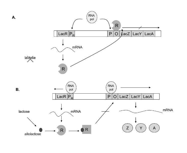
Figure 1. The lac operon. See [deBoer, , p. 37].

Figure 1 is to be interpreted as follows. In panel A no lactose is present. The repressor protein $R$ can bind to the operator region of the lac operon and block RNA polymerase from transcribing the operon genes. In panel B lactose and its isomer allolactose are present. The allolactose causes a conformational change in the repressor protein which prevents it from blocking transcription. Consequently, RNA polymerase transcribes the operon into mRNA which, in turn, is translated into the proteins $Z,Y,$ and $A$.

How is the lac operon regulated? Positive control takes place in the absence of glucose and presence of lactose in the cell. Some of the lactose is converted into allolactose, which acts as an inducer of transcription of the lac genes. This process involves the protein CAP (catabolite activator protein), which forms a complex with the substrate cAMP. This complex, in turn, binds to the activator region of the operon. Translation of the mRNA gives rise to the proteins $\beta$-galactoside permease (LacY), which transports external lactose into the cell, and $\beta$-galactosidase (LacZ), which cleaves lactose into glucose and its stereoisomer galactose. It also converts lactose into allolactose (Fig. 1.B). A third protein, LacA, is not directly involved in lactose metabolism. Transcription continues until glucose becomes available. When that happens two negative control mechanisms take over. Inside the cell, synthesis of the protein cAMP is inhibited, which is needed for transcription of the operon, and the repressor protein LacI can bind to the operator region of the lac operon, preventing transcription (Fig. 1.A). This is known as catabolite repression. Furthermore, external glucose inhibits the transport of lactose into the cell through a process called inducer exlusion. We want to emphasize that this description is very simplified and does not mention many of the biochemical mechanisms involved in this control circuit.

4. A Continuous Model

As one of the oldest known gene regulation network, the lac operon has been studied extensively and many different mathematical models have been constructed for it; see leibler . The most common type of model is based on ordinary differential equations. For a model from the recent literature see yildirim . We discuss here the very simple dynamical systems model described in Section 5.2 of the undergraduate text book deBoer . It consists of three equations, modeling the concentration of the repressor $R$ and the rates of change of the operon mRNA $M$ and allolactose $A$. The three equations are:

$$R = \frac{1}{1+A^{n}},$$

$$\frac{dM}{dt} = c_{0}+c(1-R)-\gamma M,$$

$$\frac{dA}{dt} = ML-\delta A-\frac{vMA}{h+A}.$$

Here $c_{0},c,\gamma,v,\delta,h$ and $L$ are certain model parameters, $n$ is a fixed positive integer, and the concentrations $R,M$ and $A$ are functions of time $t$.

This model is based on several assumptions. For instance, we do not distinguish between intracellular and extracellular lactose, and denote both by $L$. Another assumption is that $\beta$-galactosidase is proportional to operon activity $M$ and is not represented explicitly. The concentration of the repressor $R$ is represented by a sigmoid function, a so-called Hill function. When extracellular lactose is present and is transported to the intracellular environment by lactose permease, produced by the activity of the operon, the allolactose concentration increases and inhibits the repressor $R$. The Hill coefficient $n$ determines the shape of the sigmoidal function. The larger $n$, the steeper and more switch-like the curve becomes. As we will see, this coefficient also determines the degree of the polynomial system we need to solve. Biologically, $n$ can often be interpreted as a specific measured quantity, such as the number of molecules of a particular species that are involved in a cooperative reaction.

The rate of change of the gene transcripts $M$ is composed of a baseline activity represented by the constant $c_{0}$, the concentration $A$ of allolactose (which inhibits the repressor $R$), and a degradation term $\gamma M$. The concentration of allolactose $A$ increases with the activity $M$ of the operon genes in conjunction with the presence of lactose $L$. Its degradation (the terms on the right-hand side with minus signs) is represented by a Michaelis-Menten type enzyme substrate reaction composed of two terms. The parameters $c_{0},c,\gamma,v,\delta,h$ and $L$ need to be estimated using biological considerations or numerical methods, to ensure that the model is consistent with experimental data.

This model is also quite simplified, both from a biological and a mathematical point of view. But even a simple model can be useful. The purpose of modeling is to identify the essence of a system, that is, to identify the components and dynamics that are key to conferring the biological function. This is analogous to identifying that the key component for moving the bus forward is the engine. The art of constructing mathematical models of biological systems (or any other type of system, for that matter) is to incorporate the most important features and mechanisms and discard the irrelevant ones. Comparing the model to the Boolean network model constructed in the next section, we will see certain basic similarities, even though the mathematics is different. We have a time-discrete finite dynamical system on the one hand and a continuous-time system given by differential equations on the other hand.

It is now time to analyze the dynamics of the continuous model, by computing its steady states. We do this by phrasing the problem in a way that makes it amenable to using algebra, namely by setting the right hand sides of the differential equations to zero:

$$c_{0}\,+\,c\cdot(1-\frac{1}{1+A^{n}})\,-\,\gamma\cdot M\,\,\,\,=\,\,\,\,M\cdot L\,-\,\delta\cdot A\,-\,\frac{vMA}{h+A}\,\,\,\,=\,\,\,\,0.$$

This is a system of two algebraic equations in two variables $A$ and $M$, which depends on the various parameters. Note that the steady state values for the missing variable $R$ are determined by the equation $\,R=1/(1+A^{n})$.

Following the discussion in [deBoer, , Section 5.2], we leave the concentration $L$ of lactose unspecified while the other parameter values are fixed as follows:

$$c=\gamma=v=1,\,\,c_{0}=\frac{1}{20},\,h=2,\,m=5,\,\delta=\frac{1}{5}.$$

We also set $n=5$. Our algebraic equations now take the form

$$\frac{1}{20}\,+\,\frac{A^{5}}{1+A^{5}}-M\quad=\quad M\cdot L-\frac{1}{5}\cdot A\,-\,\frac{MA}{2+A}\quad=\quad 0.$$

By clearing denominators and eliminating the unknown $M$, we find that

$$4\,A^{7}\,+\,(29-21L)\,A^{6}\,-\,42L\,A^{5}\,+\,4\,A^{2}\,+\,(9-L)\,A\,-\,2L\,\,\,=\,\,\,0.$$

This is a polynomial of degree $7$ in $A$. The discriminant of this polynomial in $A$ is a complicated polynomial of degree $12$ in the parameter $L$. This discriminant has precisely two positive roots, which we determine to be

$$L_{1}\,=\,0.68454...\quad\hbox{and}\quad L_{2}\,=\,1.51054....$$

For all values of $L$ between $L_{1}$ and $L_{2}$, there are three positive steady states. For example, if $L=1$ then the steady states $(R,M,A)$ of our system are

$$(0.2272,0.0506,0.9994)\,,\,\,(0.6907,0.1859,0.8642)\,,\,\,(2.3717,1.0368,0.0132).$$

The above expression $\,4A^{7}+(29-21L)A^{6}+\cdots\,$ is the equation of the bifurcation diagram in the $(A,L)$-plane which is depicted in [deBoer, , Figure 5.3(b)]. It describes the steady-state allolactose concentration $A$ as a function of the lactose concentration $L$. As argued in [deBoer, , Section 5.3], the emergence of these three steady states shows that this model correctly captures key features of the lac operon. Computer algebra allows us to vary other parameters and enables us to conduct a very careful analysis of the dynamics of this model. In particular, using computer algebra, we can derive a precise algebraic description of the region in parameter space for which the dynamical system has more than one stationary point, and we can identify parameter values at which interesting phenomena (e.g. Hopf bifurcations GMS ) might occur.

5. A Discrete Model

While most models of the lac operon have used the framework of ordinary differential equations, other modeling frameworks can also be useful. We describe a discrete model, in the form of a Boolean network, taken from the recent article SV . Like most models, it is very simplified in its representation of biological details and mechanisms. But it attempts only to capture a basic dynamic feature of the lac operon, namely its bistability.

Each one of the variables in the model can take on the states 0 and 1, corresponding to the simplifying biological assumption that the role a molecular species plays in this network depends only on its absence or presence (defined by a suitably chosen threshold) rather than a more refined measure of its concentration in the cell. The model has nine variables, representing concentrations of various molecular species, some of which have already appeared in the continuous model in the previous section:

1. mRNA for the genes LacZ, LacY, and LacA ($M$) (the value of this variable indicates whether the operon is ON or OFF),

2. lac permease ($P$),

3. $\beta$-galactosidase ($B$),

4. catabolite activator protein CAP ($C$),

5. repressor protein LacI ($R$),

6. lactose ($L$) and allolactose ($A$),

7. low concentrations of lactose ($L_{\ell}$) and allolactose ($A_{\ell}$).

The two variables $L_{\ell}$ and $A_{\ell}$ are “artifical,” in the sense that, for the model to be accurate, it needs to allow for three, rather than two, possible concentration levels of lactose and allolactose: absent, low, and high. In order to avoid the use of multistate variables, we can keep the binary setting by introducing additional variables that account for low concentrations of these chemicals. The model has two parameters: external lactose $a$ and external glucose $g$. These are either present (1) or absent (0). The interactions between these molecular species are described by Boolean functions:

1. $H_{M}(t+1)\,=\,\neg R(t)\wedge C(t)$,

2. $H_{P}(t+1)\,=\,M(t)$,

3. $H_{B}(t+1)\,=\,M(t)$,

4. $H_{C}(t+1)\,=\,\neg g$,

5. $H_{R}(t+1)\,=\,\neg A(t)\wedge\neg A_{\ell}(t)$,

6. $H_{A}(t+1)\,=\,L(t)\wedge B(t)$,

7. $H_{A_{\ell}}(t+1)\,=\,A(t)\vee L(t)\vee L_{\ell}(t)$,

8. $H_{L}(t+1)\,=\,\neg g\wedge P(t)\wedge a$,

9. $H_{L_{\ell}}(t+1)\,=\,\neg g\wedge(L(t)\vee a)$.

These functions are to be interpreted as follows. The genes are transcribed ($H_{M}(t+1)=1$) at time $t+1$ if the repressor $R$ is absent and CAP is present at time $t$; permease and $\beta$-galactosidase are present at time $t+1$ if the operon is transcribed at time $t$. The interpretation of the other functions is similar. The result is a time-discrete dynamical system $\mathbf{H}(t)$, on the space of binary 9-tuples, with dynamics generated by iteration of $\mathbf{H}$. The model assumes that the molecular mechanisms leading from activation of a gene to the production of the corresponding protein (transcription plus translation) happen in one time step, as does mRNA and protein degradation.

It is shown in SV that this simple model, based on very few assumptions, displays a dynamic behavior that captures an essential feature of the lac operon, namely, its bistability. To show this, one needs to examine the long term dynamics, or steady states and periodic states, of the model. A state of the system is represented by a binary $9$-tuple $(M,P,B,C,R,A,A_{\ell},L,L_{\ell})$, such as $(1,1,1,0,1,0,0,1,1)$. If we apply the dynamical system $\mathbf{H}$ to this state, with the parameter setting $a=1,g=0$, that is, external lactose is present and external glucose is absent, we obtain the next state $(0,1,1,1,1,1,1,0,1)$. After iterating five more times we reach the state $\mathbf{u}=(1,1,1,0,1,1,1,1)$, which turns out to be a steady state, that is, $\mathbf{H}(\mathbf{u})=\mathbf{u}$. This state corresponds to the operon being ON, with all molecular species, except the repressor $R$, present. We would like to compute all such steady states $\mathbf{u}$ for the system (1)-(9).

In the case of this model it is possible to solve the resulting system of 9 equations by hand, as mentioned earlier. Alternatively, one can find the steady states by computing the value of $\mathbf{H}$ on all $2^{9}$ 9-tuples for each of the four possible parameter settings, for a total of 2048 evaluations of $\mathbf{H}$. (For instance, the software DVD can perform this computation.) For larger models it is typically not possible to do either. For example, in LM a Boolean network model of T-cell receptor signaling with 94 equations was published. In that case, we can use computational tools provided by computer algebra, which provide a systematic way to solve the system of steady state equations. The search for effective algorithms to solve very large systems of polynomial equations over finite fields, and the Boolean field in particular, is currently an active area of research (see, e.g., B ). We demonstrate their use with the lac operon model discussed here.

We first translate the Boolean functions in the model into polynomials. This uses arithmetic modulo 2. To translate a Boolean function into a polynomial function, we observe first that every Boolean function is expressed using the logical operators $\wedge,\vee$, and $\neg$. These can be translated into polynomial operations by observing that the functions $a\wedge b$ and $a\cdot b$ take on the same Boolean values for given values of the variables. That is, both functions take on the value 1 precisely if both $a$ and $b$ take on the value 1, otherwise the functions take on the value 0. Similarly, we see that $a\vee b=a+b+a\cdot b$ and $\neg a=a+1$. If we apply this dictionary to the Boolean functions in the model, while supressing the time variable, we obtain the following:

$$H_{M} = (R+1)C=RC+C,$$

$$H_{P} = M=H_{B},$$

$$H_{C} = g+1,$$

$$H_{R} = (A+1)(A_{\ell}+1)=AA_{\ell}+A+A_{\ell}+1,$$

$$H_{A} = LB,$$

$$H_{A_{\ell}} = A+L+L_{\ell}+LL_{\ell}+AL+AL_{\ell}+ALL_{\ell},$$

$$H_{L} = (g+1)aP,$$

$$H_{L_{\ell}} = (g+1)(L+aL+a).$$

A steady state of the system for a given choice of the parameters $a$ and $g$ is one for which the functions do not change the value of the variables. It is therefore a solution to the system of polynomial equations

$$H_{M}\,=\,M,\,\,\ldots,\,H_{L_{\ell}}\,=\,L_{\ell}.$$

The system in Section 2 arises for the parameter choice $g=0$ and $a=1$. Solving the system for all four possible parameter settings, $g=0=a;g=1,a=0;g=1=a;$ and $g=0,a=1$, results in the four corresponding steady states:

$$\begin{matrix}(0,0,0,1,1,0,0,0,0),&(0,0,0,0,1,0,0,0,0),\\ \,\,(0,0,0,0,1,0,0,0,0),&(1,1,1,1,0,1,1,1,1).\end{matrix}$$

The last steady state is the one we found in Section 2 and is the only one for which the lac operon is ON, in agreement with the biological system. Note that, for each parameter setting, any initialization of the system will end in the corresponding fixed point.

In SV another smaller model is presented that captures some key features of the feedback loop structure of this model and also shows the correct dynamics. The main biological conclusion drawn in SV from the models is that the dynamic behavior of the lac operon is due to properties of the network topology rather than the specific kinetics of the network that played a role in the continuous model discussed in the previous section.

6. Discussion

It is generally agreed that modern molecular biology can benefit greatly from the use of mathematical techniques that allow the construction of complex system-level models of biological networks. Conversely, the problems that arise in today’s biological research can provide important stimuli for mathematical research. This is aptly expressed in the title Mathematics is Biology’s Next Microscope, Only Better; Biology is Mathematics’ Next Physics, Only Better of cohen . We have attempted here to describe through mathematical models of the lac operon how algebra can contribute to a formal description and an analytical understanding of biological phenomena. One goal was to show that different types of mathematical models (discrete and continuous) can provide insight into biological mechanisms. Furthermore, we have demonstrated that computer algebra, not traditionally used in biology, is a powerful tool that can help construct and analyze biological models in a systematic way. Thus, this paper should be viewed as an advertisement for an in-depth study of the relationship between computer algebra, and mathematics in general, and systems biology. The marriage between the two promises to be extremely fruitful for both.

One forum for such interactions is the annual international conference series Algebraic Biology AB05 which was started in 2005. Another one is the year-long program on Algebraic Methods in Systems Biology and Statistics held at the Statistical and Applied Mathematical Sciences Institute (SAMSI) in North Carolina during the academic year 2008-09.

Several open mathematical research problems arise from our discussion. Firstly, in both Sections 3 and 4, we used computer algebra algorithms to determine solutions to systems of nonlinear polynomial equations. In one case the polynomials have real coefficients and in the other they take binary values. In the binary case, a central problem is to improve the power of the algorithms and the speed of the software implementations. Unlike the real coefficient case, relatively little work has been done until recently on the development of efficient solution methods for polynomial systems over finite fields in general, and the Boolean field in particular. Where exact solutions cannot be computed, information about the number of solutions, e.g., the number of steady states, would be of interest. Tools involving zeta functions of algebraic varieties over finite fields might be of help here. Another source of problems in computer algebra comes from the task of inferring gene regulatory networks from experimental data sets, for instance, using the technique in LS .

There are numerous open problems concerning continuous dynamical systems in systems biology. Two problems we find particularly important are the characterization of chemical reaction networks that allow bistability CFRS and the Global Attractor Conjecture for Toric Dynamical Systems CDSS .

7. Biographical sketches

Reinhard Laubenbacher is Professor of Mathematics at Virginia Tech, a professor at the Virginia Bioinformatics Institute, and Adjunct Professor in the Department of Cancer Biology at the Wake Forest University School of Medicine. His research interests include computational systems biology and cancer systems biology. With his collaborators he has pioneered the use of tools and concepts from computational algebra to model biological systems.

Bernd Sturmfels is Professor of Mathematics, Statistics and Computer Science at UC Berkeley. A leading experimentalist among mathematicians, he has authored ten books and about 180 articles, in the areas of combinatorics, algebraic geometry, symbolic computation and their applications. Sturmfels currently works on algebraic methods in statistics, optimization and computational biology. His honors include the MAA’s Lester R. Ford Award and designation as a George Polya Lecturer.

References

- [1] U. Alon: An Introduction to Systems Biology: Design Principles of Biological Circuits, Chapman and Hall, 2006.
- [2] H. Anai and K. Horimoto: Algebraic Biology 2005, Proceedings of the First International Conference on Algebraic Biology – Computer Algebra in Biology – held on November, 28–30, 2005, in Tokyo, Japan, Universal Academy Press, Tokyo, Japan.
- [3] M. Barnett: Computer algebra in the life sciences, ACM SIGSAM Bulletin, Volume 36, Issue 4 (December 2002), pp. 5–32.
- [4] M. Brickenstein, A. Dreyer, G.-M. Greuel, M. Wedler, and O. Wienand, New developments in the theory of Gröbner bases and applications to formal verification, arXiv:0801.1177.
- [5] R. D. Boer: Theoretical Biology, Undergraduate Course at Utrecht University, book posted at http://theory.bio.uu.nl/rdb/books/.
- [6] M. Casanellas and J. Fernández-Sánchez: Performance of a new invariants method on homogeneous and non-homogeneous quartet trees, Molecular Biology and Evolution 24 (2007) 288–293.
- [7] B. Cipra: Algebraic geometers see ideal approach to biology, SIAM News 40, Number 6, July/August 2007.
- [8] J. Cohen: Mathematics is biology’s next microscope, only better; biology is mathematics’ next physics, only better, PLoS Biology 2 (2004) 2017–2023.
- [9] C. Conradi, D. Flockerzi, J. Raisch and J. Stelling: Subnetwork analysis reveals dynamic featurs of complex (bio)chemical networks, PNAS 104 (2007) 19175–19180.
- [10] G. Craciun, A. Dickenstein, A. Shiu, and B. Sturmfels: Toric dynamical systems, arXiv:0708.3431.
- [11] D.A. Cox, J. Little, and D. O’Shea: Ideals, Varieties and Algorithms, Springer Verlag, New York, third edition, 2007.
- [12] F. Jacob and J. Monod: Genetic regulatory mechanisms in the synthesis of proteins, J. Molecular Biology 3 (1961) 318–356.
- [13] J. Guckenheimer, M Myers and B. Sturmfels: Computing Hopf bifurcations, SIAM J. Numerical Analysis 34 (1997) 1–21.
- [14] H. Kitano: Systems biology: a brief overview, Science 295 (2002) 1662–1664.
- [15] R. Laubenbacher, A. Jarrah, H. Vastani, and B. Stigler: Discrete Visualizer of Dynamics, http://dvd.vbi.vt.edu
- [16] R. Laubenbacher and B. Stigler: A computational algebra approach to the reverse engineering of gene regulatory networks, Journal of Theoretical Biology, 229 (2004) 523–537.
- [17] Y. Lazebnik: Can a biologist fix a radio? – or what I learned while studying apoptosis, Cancer Cell 2 (2002) 179–182.
- [18] H. Lodish, A. Berk, L. Zipursky, P. Matsudaira, D. Baltimore, and J. Darnell: Molecular Cell Biology, W.H. Freeman and Company, New York, 2000.
- [19] L. Pachter and B. Sturmfels: Algebraic Statistics for Computational Biology, Cambridge University Press, 2005.
- [20] J. Saez-Rodriguez, L. Simeoni, J. A. Lindquist, R. Hemenway, U. Bommhardt, B. Arndt U. Haus, R. Weismantel, E. D. Gilles, S. Klamt, B. Schraven: A logical model provides insights into T cell receptor signaling, PLOS Comp. Biol. 3 (8), 2007.
- [21] B. Stigler and A. Veliz-Cuba: Network topology as a driver of bistability in the lac operon, arXiv:0807.3995.
- [22] G. A. Stolovitzky, D. Monroe, and A. Califano: Dialogue on reverse engineering assessment and methods: the DREAM of high throughput pathway inference, Ann. N.Y. Acad. Sci. 1115, 2007.
- [23] B. Sturmfels: What is a Gröbner basis?, Notices of the American Mathematical Society, 52 (2005) 1199–1200.
- [24] J.M.G. Vilar, C.C. Guet, and S. Leibler: Modeling network dynamics: the lac operon, a case study, The Journal of Cell Biology 161 (2003) 471–476.
- [25] N. Yildirim and M. Mackey: Feedback regulation in the lactose operon: A mathematical modeling study and comparison with experimental data, Biophysical Journal 84 (2003) 2831–2851.