Short rational generating functions for multiobjective linear integer programming

Abstract.

This paper presents algorithms for solving multiobjective integer programming problems. The algorithm uses Barvinok’s rational functions of the polytope that defines the feasible region and provides as output the entire set of nondominated solutions for the problem. Theoretical complexity results on the algorithm are provided in the paper. Specifically, we prove that encoding the entire set of nondominated solutions of the problem is polynomially doable, when the dimension of the decision space is fixed. In addition, we provide polynomial delay algorithms for enumerating this set. An implementation of the algorithm shows that it is useful for solving multiobjective integer linear programs.

Introduction

Short rational functions were used by Barvinok [2] as a tool to develop an algorithm for counting the number of integer points inside convex polytopes, based in the previous geometrical papers by Brion [6],Khovanskii and Puhlikov [22], and Lawrence [24]. The main idea is encoding those integral points in a rational function in as many variables as the dimension of the space where the body lives. Let $P\subset\mathbb{R}^{d}$ be a given convex polyhedron, the integral points may be expressed in a formal sum $f(P,z)=\sum_{\alpha}z^{\alpha}$ with $\alpha=(\alpha_{1},\ldots,\alpha_{d})\in P\cap\mathbb{Z}^{d}$, where $z^{\alpha}=z_{1}^{\alpha_{1}}\cdots z_{d}^{\alpha_{d}}$. Barvinok’s aimed objective was representing that formal sum of monomials in the multivariate polynomial ring $\mathbb{Z}[z_{1},\ldots,z_{n}]$, as a “short” sum of rational functions in the same variables. Actually, Barvinok presented a polynomial-time algorithm when the dimension, $n$, is fixed, to compute those functions. A clear example is the polytope $P=[0,N]\subset\mathbb{R}$: the long expression of the generating function is $f(P,z)=\sum_{i=0}^{N}z^{i}$, and it is easy to see that its representation as sum of rational functions is the well known formula $\frac{1-z^{N+1}}{1-z}$.

Brion proved in 1988 [6], that for computing the short generating function of the formal sum associated to a polyhedron, it is enough to do it for tangent cones at each vertex of $P$. Barvinok applied this function to count the number of integral points inside a polyhedron $P$, that is, $\lim_{z\rightarrow(1,\ldots,1)}f(P,z)$, that is not possible to compute using the original expression, but it may be obtained using tools from complex analysis over the rational function $f$.

The above approach, apart from counting lattice points, has been used to develop some algorithms to solve, exactly, integer programming. Actually, De Loera et al [9] and Woods and Yoshida [35] presented different methods to solve this family of problems using Barvinok’s rational function of the polytope defined by the constraints of the given problem.

The goal of this paper is to present new methods for solving multiobjective integer programming problems. In contrast to usual integer programming problems, in multiobjective problems there are at least two (and in this case the problem is called biobjective) or more objective functions to be optimized.

The importance of multiobjective optimization is not only due to its theoretical implications but also to its many applications. Witnesses of that are the large number of real-world decision problems that appear in the literature formulated as multiobjective programs. Examples of them are flowshop scheduling (see  [18]), analysis in Finance (see [13], Chapter 20), railway network infrastructure capacity (see [11]), vehicle routing problems (see [20, 29]) or trip organization (see [31]).

Multiobjective programs are formulated as optimization (we restrict ourselves without lost of generality to the maximization case) problems over feasible regions with at least two objective functions. Usually, it is not possible to maximize all the objective functions simultaneously since objective functions induce a partial order over the vectors in the feasible region, so a different notion of solution is needed. A feasible vector is said to be a nondominated (or Pareto optimal) solution if no other feasible vector has componentwise larger objective values. The evaluation through the objectives of a nondominated solution is called efficient solution.

This paper studies multiobjective integer linear programs (MOILP). Thus, we assume that there are at least two objective functions involved, the constraints that define the feasible region are linear, and the feasible vectors are integers.

Even if we assume that the objective functions are also linear, there are nowadays relatively few exact methods to solve general multiobjective integer and linear problems (see [13]). Some of them, as branch and bound with bound sets, which belong to the class of implicit enumeration methods, combine optimality of the returned solutions with adaptability to a wide range of problems (see for example [36, 37, 26, 27] for details). Other methods, as Dynamic Programming, are general methods for solving, not very efficiently, general families of optimization problems (see [21, 7]). A different approach, as the Two-Phase method (see [33]), looks for supported solutions (those that can be found as solutions of a single-objective problem over the same feasible region but with objective function a linear combination of the original objectives) in a first stage and non-supported solutions are found in a second phase using the supported ones. The Two-phase method combines usual single-criteria methods with specific multiobjective techniques.

Apart from those generic methods, there are specific algorithms for solving some combinatorial biobjective problems: biobjective knapsacks ([34]), biobjective minimum spanning tree problems ([30]) or biobjective assignment problems ([28]), as well as heuristics and metaheuristics algorithms that decrease the CPU time for computing the nondominated solutions for specific biobjective problems.

Nowadays, new approaches for solving multiobjective problems, using tools from Algebraic Geometry and Computational Algebra, have been proposed in the literature aiming to provide new insights into the combinatorial structure of the problems. This new research line seems to be prolific in a near future. An example of that is presented in [5] where a notion of partial Gröbner basis is given that allows to build a test family (analogous to the test set concept but for solving multiobjective problems) to solve general multiobjective linear integer programming problems.

Another witness of this trend is the recent work by Deloera et al. [10]. In this paper, the authors present several algorithms for multiobjective integer linear programs using generating functions. Nevertheless, their approach differs from ours in that their requires, in addition, to fix the dimension of the objective space to prove polynomiality of their algorithms, and their proofs are totally different. Moreover, no actual implementation of the algorithms is shown in that paper although it addresses an interesting shortest distance problems respect to a prespecified Pareto point.

In this paper, we also use rational generating function of polytopes for solving multiobjective integer linear programs.

In Section 1, the main results on Barvinok’s rational functions, which we use in our approach, are presented. Section 2 presents the multiobjective integer problem and the notion of dominance in order to clarify which kind of solutions we are looking for. The two following sections analyze different algorithms for solving general multiobjective problems. In Section 3, fixing the dimension of the decision space, a polynomial time algorithm that encodes the set of nondominated solutions of the problem as a short sum of rational functions is detailed. Next, a digging algorithm that computes the entire set of nondominated solutions using the multivariate Laurent expansion for the Barvinok’s function of the polytope defined by the constraints of the problem is given in Section 4. In that section, a polynomial delay algorithm for solving multiobjective problems is also presented (fixing only the dimension of the decision space).

Section 5 shows the results of a computational experiment and its analysis. Here, we solve biobjective knapsack problems, report on the performance of the algorithms and draw some conclusions on their results and their implications.

1. Barvinok’s rational functions

In this section, we recall some results on short rational functions for polytopes, that we use in our development. For details the interested reader is referred to [2, 3, 4].

Let $P=\{x\in\mathbb{R}^{n}:A\,x\leq b\}$ be a rational polytope in $\mathbb{R}^{n}$. The main idea of Barvinok’s Theory was encoding the integer points inside a rational polytope in a “long” sum of monomials:

$$f(P;z)=\displaystyle\sum_{\alpha\in P\cap\mathbb{Z}^{n}}\,z^{\alpha}$$

where $z^{\alpha}=z_{1}^{\alpha_{1}}\cdots z_{n}^{\alpha_{n}}$.

The following results, due to Barvinok, allow us to re-encode, in polynomial-time for fixed dimension, these integer points in a “short” sum of rational functions.

Theorem 1.1 (Theorem 5.4 in [2]).

Assume $n$, the dimension, is fixed. Given a rational polyhedron $P\subset\mathbb{R}^{n}$ , the generating function $f(P;z)$ can be computed in polynomial time in the form

$$f(P;z)=\displaystyle\sum_{i\in I}\varepsilon_{i}\dfrac{z^{u_{i}}}{\displaystyle\prod_{j=1}^{n}(1-z^{v_{ij}})}$$

where $I$ is a polynomial-size indexing set, and where $\varepsilon\in\{1,-1\}$ and $u_{i},v_{ij}\in\mathbb{Z}^{n}$ for all $i$ and $j$.

As a corollary of this result, Barvinok gave an algorithm for counting the number of integer points in $P$. It is clear from the original expression of $f(P;z)$ that this number is $f(P;\mathbf{1})$, but $\mathbf{1}=(1,\ldots,1)$ is a pole for the rational function, so, the number of integer points in the polyhedron is $\displaystyle\lim_{z\rightarrow\mathbf{1}}f(S;z)$. This limit can be computed using residue calculation tools from elementary complex analysis.

Another useful result due to Barvinok and Wood [4], states that computing the short rational function of the intersection of two polytopes, given the respective short rational function for each polytope, is doable in polynomial time.

Theorem 1.2 (Theorem 3.6 in [4]).

Let $P_{1}$, $P_{2}$ be polytopes in $\mathbb{R}^{n}$ and $P=P_{1}\cap P_{2}$. Let $f(P_{1};z)$ and $f(P_{2};z)$ be their short rational functions with at most $k$ binomials in each denominator. Then there exists a polynomial time algorithm that computes

$$f(P;z)=\displaystyle\sum_{i\in I}\gamma_{i}\dfrac{z^{u_{i}}}{\displaystyle\prod_{j=1}^{s}(1-z^{v_{ij}})}$$

with $s\leq 2k$, where the $\gamma_{i}$ are rational numbers and $u_{i}$, $v_{ij}$ are nonzero integral vectors for $i\in I$ and $j=1,\ldots,s$.

In the proof of the above theorem, the Hadamard product of a pair of power series is used. Given $g_{1}(z)=\displaystyle\sum_{m\in\mathbb{Z}^{d}}\beta_{m}\,z^{m}$ and $g_{2}(z)=\displaystyle\sum_{m\in\mathbb{Z}^{d}}\gamma_{m}\,z^{m}$, the Hadamard product $g=g_{1}\ast g_{2}$ is the power series

$$g(z)=\displaystyle\sum_{m\in\mathbb{Z}^{n}}\eta_{m}\,z^{m}\qquad\text{where $\eta_{m}=\beta_{m}\gamma_{m}$}.$$

The following Lemma is instrumental to prove Theorem 1.2.

Lemma 1.1 (Lemma 3.4 in [4]).

Let us fix $k$. Then there exists a polynomial time algorithm, which, given functions $g_{1}(z)$ and $g_{2}(z)$ such that

(1) $$g_{1}(z)=\dfrac{z^{p_{1}}}{(1-z^{a_{11}})\cdots(1-z^{a_{1k}})}\quad and\quad g_{2}(z)=\dfrac{z^{p_{2}}}{(1-z^{a_{21}})\cdots(1-z^{a_{2k}})}$$

where $p_{i},a_{ij}\in\mathbb{Z}^{d}$ and such that there exists $l\in\mathbb{Z}^{l}$ with $\langle l,a_{ij}\rangle<0$ for all $i,j$, computes a function $h(z)$ in the form

$$h(z)=\displaystyle\sum_{i\in I}\beta_{i}\dfrac{z^{q_{i}}}{(1-z^{b_{i1}})\cdots(1-z^{b_{i}s})}$$

with $q_{i},b_{ij}\in\mathbb{Z}^{d}$, $\beta_{i}\in\mathbb{Q}$ and $s\leq 2k$ such that $h$ possesses the Laurent expansion in a neighborhood $U$ of $z_{0}=(e^{l_{1}},\ldots,e^{l_{n}})$ and $h(z)=g_{1}(z)\ast g_{2}(z)$.

For proving Theorem 1.2, it is enough to assure that for given polytopes $P_{1},P_{2}\subseteq Z^{n}$, their rational functions satisfy conditions (1). It is not difficult to ensure that the conditions are verified after some changes are done in the expressions for the short rational functions (for further details, the interested reader is referred to [4]).

Actually, with this result a general theorem can be proved ensuring that for a pair of polytopes, $P_{1},P_{2}\subseteq\mathbb{Z}^{n}$, there exists a polynomial time algorithm to compute, given the rational functions for $P_{1}$ and $P_{2}$, the short rational function of any boolean combination of $P_{1}$ and $P_{2}$.

Finally, we recall that one can find, in polynomial time, rational functions for polytopes that are images of polytopes with known rational function.

Lemma 1.2 (Theorem 1.7 in [2]).

Let us fix $n$. There exists a number $s=s(n)$ and a polynomial time algorithm, which, given a rational polytope $P\subseteq\mathbb{R}^{n}$ and a linear transformation $T:\mathbb{R}^{n}\rightarrow\mathbb{R}^{r}$ such that $T(\mathbb{Z}^{n})\subseteq\mathbb{Z}^{r}$, computes the function $f(S;z)$ for $S=T(P\cap\mathbb{Z}^{n})$, $S\subseteq\mathbb{Z}^{r}$ in the form

$$f(S;z)=\displaystyle\sum_{i\in I}\alpha_{i}\dfrac{z^{p_{i}}}{(1-z^{a_{i1}})\cdots(1-z^{a_{i}s})}$$

where $\alpha_{i}\in\mathbb{Q}$, $p_{i},a_{ij}\in\mathbb{Z}^{r}$ and $a_{ij}\neq 0$ for all $i,j$.

To finish this section, we mention the application of short rational functions to solve single-objective integer programming. The interested reader is referred to [9, 35] for further details.

2. Multiobjective combinatorial optimization problems

In this section we present the problem to be solved as well as the new concept of solutions motivated by the nature of the problem.

A multiobjective integer linear program (MOILP) can be formulated as:

$$\max \;(c_{1}\,x,\ldots,c_{k}\,x)=:C\,x$$

$$s.t.$$

(2) $$\displaystyle\sum_{j=1}^{d}\,a_{ij}\,x_{j}\leq b_{i} i=1,\ldots,m$$

$$x_{j}\in\mathbb{Z}_{+} j=1,\ldots,n$$

with $a_{ij},b_{i}$ integers and $x_{i}$ non negative. Without loss of generality, we will consider the above problem in its standard form, i.e., the coefficient of the $k$ objective functions are non-negative and the constraints are in equation form. In addition, we will assume that the constraints define a polytope (bounded) in $\mathbb{R}^{n}$. Therefore, from now on we deal with $MOILP_{A,C}(b)$.

It is clear that Problem (2) is not a standard optimization problem since the objective function is a $k$-coordinate vector, thus inducing a partial order among its feasible solutions. Hence, solving the above problem requires an alternative concept of solution, namely the set of nondominated (or Pareto-optimal) points.

A vector $\widehat{x}\in\mathbb{R}^{n}$ is said to be a nondominated (or Pareto optimal) solution of $MIOLP_{A,C}$ if there is no other feasible vector $y$ such that

$$c_{j}\,y\geq c_{j}\,\widehat{x}\qquad\forall j=1,\ldots,k$$

with at least one strict inequality for some $j$. If $x$ is a nondominated solution, the vector $Cx=(c_{1}\,x,\ldots,c_{k}\,x)\in\mathbb{R}^{k}$ is called efficient. Note that $X_{E}$ is a subset of $\mathbb{R}^{n}$ (decision space) and $Y_{E}$ is a subset of $\mathbb{R}^{k}$ (objectives space).

We will say that a dominated point, $y$, is dominated by $x$ if $c_{i}\,x\gvertneqq c_{i}\,y$ for all $i=1,\ldots,k$. We denote by $X_{E}$ the set of all nondominated solutions for (2) and by $Y_{E}$ the image under the objective functions of $X_{E}$, that is, $Y_{E}=\{C\,x:x\in X_{E}\}$.

From the objective function $C$, we obtain a linear partial order on $\mathbb{Z}^{n}$ as follows:

$$x\succ_{C}y:\Longleftrightarrow C\,x\gvertneqq C\,y$$

Notice that since $C\in\mathbb{Z}^{k\times n}$, the above relation is not complete. Hence, there may exist non-comparable vectors. We will use this partial order, induced by the objective functions of problem (2) as the input for the multiobjective integer programming algorithm developed in this paper.

Sometimes, the same efficient value is the image of several nondominated solutions. At this point, different problems can be tackled. We say that two nondominated solutions, $x^{1}$ and $x^{2}$ are equivalent if $C\,x^{1}=C\,x^{2}$. Then, the solutions for $MOILP_{A,C}(b)$ are one of the following:

• Complete set: A subset $X\subseteq X_{E}$ such that for all $y\in Y_{E}$ there is $x\in X$ with $C\,x=y$.

• Minimal complete set: A complete set with no equivalent solutions.

• Maximal complete set: All equivalent solutions.

Through this paper, we are looking for the entire set of nondominated solutions, equivalently the maximal complete set for $MOILP_{A,C}$.

3. A short rational function expression of the entire set of nondominated solutions

We present in this section an algorithm for solving $MOILP_{A,C}(b)$ using Barvinok’s rational functions technique.

Theorem 3.1.

Let $A\in\mathbb{Z}^{m\times n}$, $b\in\mathbb{Z}^{m}$, $C=(c_{1},\ldots,c_{k})\in\mathbb{Z}^{k\times n}$, $J\in\{1,\ldots,n\}$, and assume that the number of variables $n$ is fixed. Suppose $P=\{x\in\mathbb{R}^{n}:A\,x\leq b,x\geq 0\}$ is a rational convex polytope in $\mathbb{R}^{n}$. Then, we can encode, in polynomial time, the entire set of nondominated solutions for $MOILP_{A,C}(b)$ in a short sum of rational functions.

Proof.

Using Barvinok’s algorithm, compute the following generating function in $2n$ variables:

(3) $$f(x,y):=\displaystyle\sum_{(u,v)\in P_{C}\cap\mathbb{Z}^{2n}}x^{u}\,y^{v}$$

where $P_{C}=\{(u,v)\in\mathbb{Z}^{n}\times\mathbb{Z}^{n}:u,v\in P,c_{i}\,u-c_{i}\,v\geq 0\text{ for all $i=1,\ldots,k$ and}\displaystyle\sum_{i=1}^{k}c_{i}\,u-\displaystyle\sum_{i=1}^{k}c_{i}\,v\geq 1\}$. $P_{C}$ is clearly a rational polytope. For fixed $u\in\mathbb{Z}^{n}$, the $y$-degrees, $\alpha$, in the monomial $x^{u}\,y^{\alpha}$ of $f(x,y)$ represent the solutions dominated by $u$.

Now, for any function $\varphi$, let $\pi_{1,\varphi},\pi_{2,\varphi}$ be the projections of $\varphi(x,y)$ onto the $x$- and $y$-variables, respectively. Thus $\pi_{2,f}(y)$ encodes all dominated feasible integral vectors (because the degree vectors of the $x$-variables dominate them, by construction), and it can be computed from $f(x,y)$ in polynomial time by Lemma 1.2.

Let $V(P)$ be the set of extreme points of the polytope $P$ and choose an integer $R\geq\max\{v_{i}:v\in V(P),i=1,\ldots,n\}$ (we can find such an integer $R$ via linear programming). For this positive integer, $R$, let $r(x,R)$ be the rational function for the polytope $\{u\in\mathbb{R}^{n}_{+}:u_{i}\leq R\}$, its expression is:

$$r(x,R)=\displaystyle\prod_{i=1}^{n}\left(\dfrac{1}{1-x_{i}}+\dfrac{x_{i}^{R}}{1-x_{i}^{-1}}\right).$$

Define $f(x,y)$ as above, $\pi_{2,f}(x)$ the projection of $f$ onto the second set of variables as a function of the $x$-variables and $F(x)$ the short generating function of $P$. They are computed in polynomial time by Lemma 1.2 and Theorem 1.1 respectively. Compute the following difference:

$$h(x):=F(x)-\pi_{2,f}(x).$$

This is the sum over all monomials $x^{u}$ where $u\in P$ is a nondominated solution, since we are deleting, from the total sum of feasible solutions, the set of dominated ones.

This construction gives us a short rational function associated with the sum over all monomials with degrees being the nondominated solutions for $MOILP_{A,C}(b)$. As a consequence, we can compute the number of nondominated solutions for the problem. The complexity of the entire construction being polynomial since we only use polynomial time operations among four short rational functions of polytopes (these operations are the computation of the short rational expressions for $f(x,y)$, $r(x,R)$ and $\pi_{2,f}(x)$). ∎

Remark 3.1.

To prove the above result one can use a different approach to compute the nondominated solutions assuming that there exists a polynomially bounded (for fixed dimension) feasible lower bound set, $L$, for $MOILP_{A,C}(b)$, i.e., a set of feasible solutions such that every nondominated solution is either one element in $L$, or it dominates at least one the elements in $L$.

First, compute the following operations with generating functions:

$$H(x,y)=f(x,y)-f(x,y)*(\pi_{2,f}(x)\,r(y,R))$$

This is the sum over all monomials $x^{u}\,y^{v}$ where $u,v\in P$, $u$ is a nondominated solution and $v$ is dominated by $u$. In $H(x,y)$, each nondominated solution, $u$, appears as many times as the number of feasible solutions that it dominates.

Next, compute a feasible lower bound set (see [16, 15]), $L=\{\alpha_{1},\ldots,\alpha_{s}\}$. This way the set of nondominated solutions is encoded using the following construction:

Let $RLB^{i}(x,y)$ be the following short sum of rational functions

$$RLB^{i}(x,y)=H(x,y)\ast(y^{\alpha_{i}}\,r(x,R))\qquad i=1,\ldots,s.$$

Taking into account that for each $i$, the element $y^{\alpha_{i}}$ is common factor for $RLB^{i}(x,y)$ and it is the unique factor where the $y$-variables appear, we can define $ND^{i}(x)=\dfrac{RLB^{i}(x,y)}{y^{\alpha_{i}}},i=1,\ldots,s$, to be the sum of rational functions that encodes the nondominated solutions that dominate $\alpha_{i}$, $i=1,\ldots,s$. Therefore, the entire set of nondominated solutions for $MOILP_{A,C}(b)$ is encoded in the short sum of rational functions $ND(x)=\displaystyle\sum_{i=1}^{k}\,ND^{i}(x)$.

4. Digging algorithm for the set of nondominated solutions of MOILP

Section 3 proves that encoding the entire set of efficient solutions of MOILP can be done in polynomial time for fixed dimension. This is a compact representation of the solution concept. Nevertheless, one may be interested in an explicit description of this list of points. This task could be performed, by expanding the short rational expression which is ensured by Theorem 3.1, but it would require the implementation of all operations used in the proof. As far we know, they have never been efficiently implemented.

An alternative algorithm for enumerating the nondominated solutions of a multiobjective integer programming problem, which uses rational generating functions, is the digging algorithm. This algorithm is an extension of a heuristic proposed by Lasserre [23] for the single-objective case.

Let $A,C$ and $b$ be as in Problem (2), and assume that $P=\{x\in\mathbb{R}^{n}:Ax\leq b,x\geq 0\}$ is a polytope. Then, by Theorem 1.1, we can compute a rational expression for $f(P;z)=\sum_{\alpha\in P\cap\mathbb{Z}^{n}}z^{\alpha}$ in the form

$$f(P;z)=\displaystyle\sum_{i\in I}\varepsilon_{i}\dfrac{z^{u_{i}}}{\displaystyle\prod_{j=1}^{n}(1-z^{v_{ij}})}$$

in polynomial time for fixed dimension, $n$. Each addend in the above sum will be referred to as $f_{i}$, $i\in I$.

If we make the substitution $z_{i}=z_{i}\,t_{1}^{c_{1i}}\cdots t_{k}^{c_{ki}}$, in the monomial description we have $f(P;z,t_{1},\ldots,t_{k})=\displaystyle\sum_{\alpha\in P\cap\mathbb{Z}^{n}}z^{\alpha}\,t_{1}^{c_{1}\alpha}\cdots t_{k}^{c_{k}\alpha}$, where $c_{1},\ldots,c_{k}$ are the rows in $C$. It is clear that for enumerating the entire set of nondominated solutions, it would suffice to look for the set of leader terms, in the $t$-variables, in the partial order induced by $C$, $\succ_{C}$, of the multi-polynomial $f(P;z,t_{1},\ldots,t_{k})$. After the above changes we have:

(4) $$f(P;z,t_{1},\ldots,t_{k})=\displaystyle\sum_{i\in I}f_{i}(P;z,t_{1},\ldots,t_{k}),$$

where $f_{i}(P;z,t_{1},\ldots,t_{k}):=\varepsilon_{i}\dfrac{z^{u_{i}}\,t_{1}^{c_{1}u_{i}}\cdots t_{k}^{c_{k}u_{i}}}{\displaystyle\prod_{j=1}^{n}(1-z^{v_{ij}}\,t_{1}^{c_{1}v_{ij}}\cdots t_{k}^{c_{k}v_{ij}})}.$ Now, we can assume, wlog, that $c_{1}\,v_{ij}$ is negative or zero. If it were zero, then we could assume that $c_{2}\,v_{ij}$ is negative. Otherwise, we would repeat the argument until the first non zero element is found (it is assured that this element exists, otherwise the factor would not appear in the expression of the short rational function). Indeed, if the first non zero element were positive, we would make the change:

$$\dfrac{1}{1-z^{v_{ij}}\,t_{1}^{c_{1}v_{ij}}\cdots t_{k}^{c_{k}v_{ij}}}=\dfrac{-z^{-v_{ij}}\,t_{1}^{-c_{1}v_{ij}}\cdots t_{k}^{-c_{k}v_{ij}}}{1-z^{-v_{ij}}\,t_{1}^{-c_{1}v_{ij}}\cdots t_{k}^{-c_{k}v_{ij}}}$$

and the sign of the $t_{1}$-degree would be negative.

With these assumptions, the multivariate Laurent series expansion for each rational function, $f_{i}$, in $f(P;z,t_{1},\ldots,t_{k})$ is

$$\varepsilon_{i}z^{u_{i}}\,t_{1}^{c_{1}u_{i}}\cdots t_{k}^{c_{k}u_{i}}\displaystyle\prod_{j=1}^{d}\displaystyle\sum_{\lambda=0}^{\infty}z^{\lambda v_{ij}}t_{1}^{\lambda c_{1}v_{ij}}\cdots t_{k}^{\lambda c_{k}v_{ij}}=\varepsilon_{i}z^{u_{i}}\,t_{1}^{c_{1}u_{i}}\cdots t_{k}^{c_{k}u_{i}}\displaystyle\prod_{j=1}^{d}(1+z^{v_{ij}}t_{1}^{c_{1}v_{ij}}\cdots t_{k}^{c_{k}v_{ij}}+z^{2v_{ij}}t_{1}^{2c_{1}v_{ij}}\cdots t_{k}^{2c_{k}v_{ij}}+\cdots)$$

The following result allows us to develop a finite algorithm for solving $MOILP_{A,C}(b)$ using Barvinok’s rational generating functions.

Lemma 4.1.

Obtaining the entire set of nondominated solutions for a MOILP requires only an explicit finite, polynomially bounded (in fixed dimension) number of terms of the long sum in the Laurent expansion of $f(P;z,t_{1},\ldots,t_{k})$.

Proof.

Let $i\in I$, $j\in\{1,\ldots,n\}$ and define $P_{i}=\{\lambda\in\mathbb{Z}^{n}_{+}:c_{s}u_{i}+\displaystyle\sum_{r=1}^{n}\lambda_{r}\,c_{s}\,v_{ir}\geq 0,s=1,\ldots,k\}$, $M_{ij}=\max\{\lambda_{j}:\lambda\in P_{i}\}$ and $m_{ij}=\min\{\lambda_{j}:\lambda\in P_{i}\}$. $M_{ij}$ and $m_{ij}$ are well-defined because $P_{i}$, defined above, is non empty and bounded since, by construction, for each $j\in\{1,\ldots,n\}$ there exists $s\in\{1,\ldots,k\}$ such that $c_{s}\,v_{ij}<0$.

Then, it is enough to search for the nondominated solutions in the finite sum

$$\varepsilon_{i}z^{u_{i}}\,t_{1}^{c_{1}u_{i}}\cdots t_{k}^{c_{k}u_{i}}\displaystyle\prod_{j=1}^{d}\displaystyle\sum_{\lambda=m_{ij}}^{M_{ij}}t_{1}^{\lambda c_{1}v_{ij}}\cdots t_{k}^{\lambda c_{k}v_{ij}}.$$

Let $U$ (resp. $l$) be the greatest (resp. smallest) value that appears in the non-zero absolute values of the entries in $A$, $b$, $C$. Set $M=\max\{U,l^{-1}\}$. First, $m_{ij}\geq 0$. Then, by applying Cramer’s rule one can see that $M_{ij}$ is bounded above by $O(M^{2n+1})$. Thus, the explicit number of terms in the expansion of $f_{i}$, namely $\displaystyle\prod_{j=1}^{n}\lfloor M_{ij}-m_{ij}\rfloor$, is polynomial, when the dimension, $n$ is fixed. ∎

The digging algorithm looks for the leader terms in the $t$-variables, with respect to the partial order induced by $C$. At each rational function (addends in the above sum (4)) multiplications are done in lexicographical order in their respective bounded hypercubes. If the $t$-degree of a specific multiplication is not dominated by one of the previous factors, it is kept in a list; otherwise the algorithm continues augmenting lexicographically the lambdas. To simplify the search at each addend, the following consideration can be taken into account: if $t_{1}^{\alpha_{o}+\sum_{j}\lambda_{j}\alpha^{1}_{j}}\cdots t_{k}^{\alpha_{o}+\sum_{j}\lambda_{j}\alpha^{k}_{j}}$ is dominated, then any term of the form $t_{1}^{\alpha_{o}+\sum_{j}\mu_{j}\alpha^{1}_{j}}\cdots t_{k}^{\alpha_{o}+\sum_{j}\mu_{j}\alpha^{k}_{j}}$, $\mu$ being componentwise larger than $\lambda$, is dominated as well.

The above process is done on each rational function that appears in the representation of $f$. As an output we get a set of leader terms (for each rational function), that are the candidates to be nondominated solutions. Terms that appear with opposite signs will be cancelled. Removing terms in the list of candidates (to be nondominated solutions) implies consideration of those terms that were dominated by the cancelled ones. These terms are included in the current list of candidates and the process continues until no more terms are added.

At the end, some dominated elements may appear in the union of the final list. Deleting them in a simple cleaning process gives the list that contains only the entire set of nondominated solutions for the multiobjective problem.

Algorithm 1 details the pseudocode of the digging algorithm.

input : $A\in\mathbb{Z}^{m\times n}$, $b\in\mathbb{Z}^{m}$, $C\in\mathbb{Z}^{k\times n}$

Step 1: (Initialization)

Compute, $f(z)$, the short sum of rational functions encoding the set of nondominated solutions of $MOILP_{A,C}(b)$. The number of rational function is indexed by $I$.

Make the substitution $z_{i}=z_{i}\,t_{1}^{c_{1i}}\cdots t_{k}^{c_{ki}}$ in $f(z)$. Denote by $f_{i}$, $i\in I$, each one of the addends in $f$, as in (4).

Set $m_{ij}$ and $M_{ij}$, $j=1,\ldots,n$, the lower and upper bounds computed in the proof of Lemma 4.1 and $\mathcal{S}=\displaystyle\prod_{j=1}^{n}[m_{ij},M_{ij}]\cap\mathbb{Z}^{n}_{+}$. Set $\Gamma_{i}:=\{\}$, $i\in I$, the initial set of nondominated solutions encoded in $f_{i}$.

Step 2: (Nondominance test)

repeat 

for $i\in I$ do 

for $\lambda^{i}\in\mathcal{S}$ such that its entries are not componentwise larger than a previous $\lambda$ do 

Compute $p_{i}:=z^{w_{o}}\,t_{1}^{w_{1}}\cdots t_{k}^{w_{k}}$, being $w_{o}:=u_{i}+\,\displaystyle\sum_{j=1}^{n}\,\lambda^{i}_{j}\,v_{ij}$ and $w_{h}:=c_{1}\,u_{i}+\,\displaystyle\sum_{j=1}^{n}\,\lambda^{i}_{j}\,c_{h}\,v_{ij}\qquad h=1,\ldots,k$

if $p$ is nondominated by elements in $\Gamma_{i}$ then $\Gamma_{i}\leftarrow\Gamma_{i}\cup\{p\}$endend

Step 3: (Feasibility test)

for $s,r\in I$, $s<r$ do 

if $p\in\Gamma_{j}\cap\Gamma_{h}$, $\varepsilon_{j}=-\varepsilon_{h}$ then $\Gamma_{j}\leftarrow\Gamma_{j}\setminus\{p\}$; $\Gamma_{h}\leftarrow\Gamma_{h}\setminus\{p\}$end

until No changes in any $\Gamma_{i}$ are done for all $i\in I$ ;

Set $\Gamma:=\displaystyle\bigcup_{j}\Gamma_{j}$. Remove from $\Gamma$ the dominated elements.

output : The entire set of nondominated solutions for $MOILP_{A,C}(b)$: $\Gamma$

Algorithm 1 Digging algorithm for multiobjective problems

Recall that $M=\max\{U,l^{-1}\}$, where $U$ is the greatest value that appears in the non-zero absolute values of the entries in $A$, $b$, $C$ and $l$ is the least value among these values.

Taking into account Lemma 4.1 and the fact that Algorithm 1 never cycles, we have the following statement.

Theorem 4.1.

Algorithm 1 computes in a finite (bounded on $M$) number of steps, the entire set of nondominated solutions of the multiobjective Problem (2).

It is well known that enumerating the nondominated solutions of MOILP is NP-hard and $\#$P-hard ([12, 14]). Thus, one cannot expect to have very efficient algorithms for solving the general problem (when the dimension is part of the input).

In the following, we concentrate on a different concept of complexity that has been already used in the literature for slightly different problems. Computing maximal independent sets on graphs is known to be $\#$P-hard ([17]), nevertheless there exist algorithms for obtaining these sets which ensure that the number of operations necessary to obtain two consecutive solutions of the problem is bounded by a polynomial in the problem input size (see e.g. [32]). These algorithms are called polynomial delay. Formally, an algorithm is said polynomial delay if the delay, which is the maximum computation time between two consecutive outputs, is bounded by a polynomial in the input size ([1, 19]).

In our case, a polynomial delay algorithm, in fixed dimension, for solving a multiobjective linear integer program means that once the first nondominated solution is computed, either in polynomial time a next nondominated solution is found or the termination of the algorithm is given as an output.

Next, we present a polynomial delay algorithm, in fixed dimension, for solving multiobjective integer linear programming problems. This algorithm combines the theoretical construction of Theorem 3.1 and a digging process in the Laurent expansion of the short rational functions of the polytope associated with the constraints of the problem.

The algorithm proceeds as follows.

Let $f(z)$ be the short rational function that encodes the nondominated solutions (by Theorem 3.1, the complexity of computing $f$ is polynomial -in fixed dimension-). Make the changes $z_{i}=z_{i}\,t_{1}^{c_{1i}}\cdots t_{k}^{c_{ki}}$, for $i\in I$, in $f$. Denote by $f_{i}$ each of the rational functions of $f$ after the above changes. Next, the Laurent expansion over each rational function, $f_{i}$, is done in the following way: (1) Check if $f_{i}$ contains nondominated solutions computing the Hadamard product of $f_{i}$ with $f$. If $f_{i}$ does not contain nondominated solutions, discard it and set $I:=I\backslash\{i\}$ (termination); (2) if $f_{i}$ encodes nondominated solutions, look for an arbitrary nondominated solution (expanding $f_{i}$); (3) once the first nondominated solution, $\alpha$, is found, check if there exist more nondominated solutions encoded in the same rational function computing $f\ast(f_{i}-z^{\alpha}\,t_{1}^{c_{1}\alpha}\cdots t_{k}^{c_{k}\alpha})$. If there are more solutions encoded in $f_{i}$, look for them in $f_{i}-z^{\alpha}\,t_{1}^{c_{1}\alpha}\cdots t_{k}^{c_{k}\alpha}$. Repeat this process until no new nondominated solutions can be found in $f_{i}$.

The process above describes the pseudocode written in Algorithm 2.

input : $A\in\mathbb{Z}^{m\times n}$, $b\in\mathbb{Z}^{m}$, $C\in\mathbb{Z}^{k\times n}$

output : The entire set of nondominated ($X_{E}$) and efficient ($Y_{E}$) solutions for $MOILP_{A,C}(b)$

Set $X_{E}=\{\}$ and $Y_{E}=\{\}$.

Step 1: Compute, $f(z)$, the short sum of rational functions encoding the set of nondominated solutions of $MOILP_{A,C}(b)$. The number of rational functions is indexed by $I$.

Make the substitution $z_{i}=z_{i}\,t_{1}^{c_{1i}}\cdots t_{k}^{c_{ki}}$ in $f(z)$. Denote by $f_{i}$, $i\in I$, each one of the addends in $f$ ($f=\displaystyle\sum_{i\in I}f_{i}$).

Step 2: For each $i\in I$, check $f_{i}\ast f$. If the set of lattice points encoded by this rational function is empty, do $I\leftarrow I\setminus\{i\}$.

Step 3:

while $I\neq\emptyset$ do  for $i\in I$ do  Look for the first nondominated solution, $\alpha$, that appears in the Laurent expansion of $f_{i}$.

Set $X_{E}\leftarrow X_{E}\cup\{\alpha\}$ and $Y_{E}\leftarrow Y_{E}\cup\{C\,\alpha\}$.

Set $f_{i}\leftarrow f_{i}-z^{\alpha}\,t_{1}^{c_{1}\alpha}\cdots t_{k}^{c_{k}\alpha}$

and check if $f\ast f_{i}$ encodes lattice points. If it does not encode lattice points, discard $f_{i}$ ($I\leftarrow I\setminus\{i\}$) since $f_{i}$ does not encode any other nondominated point, otherwise repeat. endend

Algorithm 2 A polynomial delay algorithm for solving MOILP

Theorem 4.2.

Assume $n$ is a constant. Algorithm 2 provides a polynomial delay procedure to obtain the entire set of nondominated solutions of $MOILP_{A,C}(b)$.

Proof.

Let $f$ be the rational function that encodes the nondominated solutions of $MOILP_{A,C}(b)$. Theorem 3.1 ensured that $f$ is a sum of short rational functions that can be computed in polynomial time.

Algorithm 2 digs separately on each one of the rational functions $f_{i}$, $i\in I$,that define $f$. (Recall that $f=\displaystyle\sum_{i\in I}f_{i}$).

Fix $i\in I$. First, the algorithm checks whether $f_{i}$ encodes some nondominated solutions. This test is doable in polynomial time by Theorem 1.2. If the answer is positive, an arbitrary nondominated solution is found among those encoded in $f_{i}$. This is done using digging and the Intersection Lemma. Specifically, the algorithm expands $f_{i}$ on the hyperbox $\displaystyle\prod_{j=1}^{n}[m_{ij},M_{ij}]\cap\mathbb{Z}^{n}$ and checks whether each term is nondominated. The expansion is polynomial, for fixed $n$, since the number of terms is polynomially bounded by Lemma 4.1. The test is performed using the Hadamard product of each term with $f$.

The process is clearly a polynomial delay algorithm. We use digging separately on each rational function $f_{i}$ that encodes nondominated points. Thus, the time necessary to find a new nondominated solution from the last one is bounded by the application of digging on a particular $f_{i}$ which, as argued above, is polynomially bounded. ∎

Instead of the above algorithm one can use a binary search procedure to solve multiobjective problem using short generating functions. In the worst case, digging algorithm may need to expand every nonnegative term to obtain the set of nondominated solutions. Therefore, as it is stated in Theorem 4.1, the number of steps to solve the problem can be polynomially bounded on $M$. With a binary search approach, the number of steps to obtain consecutive solutions of our problem decreases to a number polynomially bounded on $log(M)$. A binary search approach was already used in [10]. Here, the novelty is that our analysis does not require to fix the dimension of the objective space whereas in [10] it was required.

The process is as follows. Let $M$ be defined as above. By construction $P\subseteq[0,M]^{n}$. We proceed by dividing the hypercube $[0,M]^{n}$ into $2^{n}$ hypercubes of smaller dimensions, and recursively repeating the division process over those hypercubes containing at least one nondominated solution (until only one solution is included in each element of the partition), whereas those hypercubes that at a given stage of the process do not contain nondominated solutions are discarded for any further consideration.

The division process is done by bisecting each dimension. Testing for nondominated solutions on a given hypercube (at any stage of the process) is always done using the same tool based on Theorem 3.1. That result allows us to construct, in polynomial time in fixed dimension, the function $h(x)$ that encodes all nondominated solutions. Moreover, it is easy to see that the short rational function that encodes the integer points in the hypercube $\mathcal{H}=\displaystyle\prod_{i=1}^{n}[m_{i},M_{i}]$, with $m_{i},M_{i}\in\mathbb{Q}$, $i=1,\ldots,n$, is:

$$r_{\mathcal{H}}(x)=\displaystyle\prod_{i=1}^{n}\big{[}\dfrac{x_{i}^{m_{i}}}{1-x_{i}}+\dfrac{x_{i}^{M_{i}}}{1-x_{i}^{-1}}\big{]}$$

Thus, the Hadamard product, $h(x)\ast r_{\mathcal{H}}(x)$ encodes the subset of nondominated solutions that lie in $\mathcal{H}$; and hence by Barvinok’s theory we can also count, in polynomial time, the number of integer points encoded by $h(x)\ast r_{\mathcal{H}}(x)$ (Lemma 3.4 in [4]).

The elements in our search space (hypercubes) are organized on a search tree and we use a depth first search strategy. Each node is a hypercube containing nondominated solutions. Descendants of a given node are hypercubes obtained bisecting the edges on the previous one (parent). It is clear that the maximum depth of the tree is $O(logM)$. The above construction ensures that, provided that the set of nondominated solutions is nonempty, finding a first nondominated solution can be done testing at most $O(2^{n}logM)$ nodes in the search tree. Since testing a node is polynomial, in fixed dimension, this operation is polynomial. Moreover, finding a new nondominated solution from a given one is also polynomial. Indeed, it consists of backtracking at most $O(logM)$ nodes until we find a branch containing nondominated points and then we have to explore, at most, $O(2^{n}logM)$ nodes; or detecting that none of the branches contain solutions.

An illustrative example of this procedure is shown in Figure 1 where can be seen how the initial hypercube, $[0,4]\times[0,4]$, is divided successively in sub-hypercubes, until an isolated nondominated solution is located in one of them.

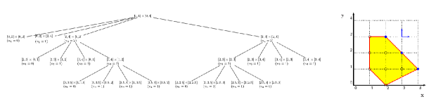
Figure 1. Search tree for the problem $v-\max\{(x,y):x+y\leq 5,x-2y\leq 2,x+y\geq 2,x\geq 1,y\leq 3,x,y\in\mathbb{Z}_{+}\}$

The finiteness of this procedure is assured since the number of times that the hypercube $[0,M]^{n}$ can be divided in $2^{n}$ sub-hypercubes is bounded by $log(M)$.

The pseudocode for this procedure is shown in Algorithm 3.

Initialization: $\mathcal{M}=[0,M]^{n}\subseteq P$.

Step 1: Let $\mathcal{M}_{1},\ldots,\mathcal{M}_{2^{n}}$ be the hypercubes obtained dividing $\mathcal{M}$ by its central point.

$i=1$

Step 2: repeat  Count $n_{\mathcal{M}_{i}}$, the number of integer points encoded in $r_{\mathcal{M}_{i}}(x)\ast h(x)$. This is the number of nondominated solutions in the hypercube $\mathcal{M}_{i}$.

if $n_{\mathcal{M}_{i}}=0$ then 

if $i<2^{n}$ then $i\leftarrow i+1$

else Go to Step 1 with $\mathcal{M}$ the next element in the search tree, using depth first search.else if $n_{\mathcal{M}_{i}}=1$ ( and $P\cap\mathcal{M}_{i}=\{x^{*}\}$) then  $ND=ND\cup\{x^{*}\}$ and $i\leftarrow i+1$. else  Go to Step 1 with $\mathcal{M}=\mathcal{M}_{i}$. enduntil $i\leq 2^{n}$ ;

Algorithm 3

Theorem 4.3.

Assume $n$ is a constant. Algorithm 3 provides a polynomial delay (polynomially bounded on $log(M)$) procedure to obtain the entire set of nondominated solutions of $MOILP_{A,C}(b)$.

Remark 4.1.

The application of the above algorithm to the single criterion case provides an alternative proof of polynomiality for the problem of finding an optimal solution of integer linear problems, in fixed dimension.

Assume that the number of objectives, $k$, is $1$, and that there exists a unique optimal value for the problem. Applying Theorem 3.1 ensures that the optimal solution of the problem is found in polynomial time, if the dimension $n$ is fixed.

Remark 4.2 (Optimization over the set of nondominated solutions).

In practice, a decision maker expects to be helped by the solutions of the multiobjective problem. In many cases, the set of nondominated solutions is too large to make easily the decision, so it is necessary to optimize (using a new criterion) over the set of nondominated solutions.

With our approach, we are able to compute, in polynomial time for fixed dimension, a “short sum of rational functions”-representation, $F(z)$, of the set of nondominated solutions of $MOILP_{A,C}(b)$. This representation allows us to re-optimize with a linear objective, $\nu$, based in the algorithms for solving single-objective integer programming problems using Barvinok’s functions (see e.g. [35]) or the algorithm proposed in Remark 4.1. The above discussion proves that solving the problem of optimizing a linear function over the efficient region of a multiobjective problem $MOILP_{A,C}(b)$ is doable in polynomial time, for fixed dimension.

5. Computational Experiments

For illustrative propposes, a series of computational experiments have been performed in order to evaluate the behavior of a simple implementation of the digging algorithm (Algorithm 1). Computations of short rational functions have been done with Latte v1.2 [8] and Algorithm 1 has been coded in MAPLE 10 and executed in a PC with an Intel Pentium 4 processor at 2.66Gz and 1 GB of RAM. The implementation has been done in a symbolic programming language, available upon request, in order to make the access easy for the interested readers.

The performance of the algorithm was tested on randomly generated instances for biobjective (two objectives) knapsack problems. Problems from 4 to 8 variables were considered, and for each group, the coefficients of the constraint were randomly generated in $[0,20]$. The coefficients of the two objective matrices range in $[0,20]$ and the coefficients of the right hand side were randomized in $[20,50]$. Thus, the problems solved are in the form:

(5) $$\max\,(c_{1},c_{2})\,x\quad s.t.\quad a_{1}x_{1}+\cdots+a_{n}\,x_{n}\leq b,x_{i}\in\mathbb{Z}_{+}$$

The computational tests have been done on this way for each number of variables: (1) Generate 5 constraint vectors and right hand sides and compute the shorts rational functions for each of them; (2) Generate a random biobjective matrix and run digging algorithm for them to obtain the set of nondominated solutions.

Table 1 contains a summary of the average results obtained for the considered knapsack multiobjective problems. The second and third columns show the average CPU times for each stage in the Algorithm: srf is the CPU time for computing the short rational function expression for the polytope with LattE and mo-digging the CPU time for running the multiobjective digging algorithm for the problem. The total average CPU times are summarized in the total column. Columns latpoints and nosrf represent the number of lattice points in the polytope and the number of short rational functions, respectively. The average number of efficient solutions that appear for the problem is presented under effic. The problems have been named as knapN where N is the number of variables of the biobjective knapsack problem.

problem	srf	latpoints	nosrf	mo-digging	effic	total
knap4	0.018	12.25	25.75	4.863	4.5	4.881
knap5	0.038	31	62.5	487.640	9.25	487.678
knap6	0.098	217.666	124.25	2364.391	7.666	2364.489
knap7	0.216	325	203	2869.268	20	2869.484
knap8	0.412	3478	342	10245.533	46	10245.933

Table 1. Summary of computational experiments for knapsack problems

As can be seen in Table 1, the computation times are clearly divided into two steps (srf and mo-digging), being the most expensive the application of the digging algorithm (Algorithm 1). In all cases more than 99% of the total time is spent expanding the short rational function using “digging algorithm”.

The CPU times and sizes in the two steps are highly sensitive to the number of variables. It is clear that one cannot expect fast algorithm for solving MOILP, since all these problems are NP-hard and #P-hard. Nevertheless, this approach gives exact tools for solving any MOILP problem, independently of the combinatorial nature of the problem.

Finally, from our computational experiments, we have detected that an easy, promising heuristic algorithm could be obtained truncating the expansion at each rational function. That algorithm would accelerate the computational times at the price of obtaining only heuristics nondominated points.

References

- [1] Arimura, H., Uno, T. (2005). A Polynomial Space and Polynomial Delay Algorithm for Enumeration of Maximal Motifs in a Sequence. ISAAC 2005: 724–737
- [2] Barvinok, A. A polynomial time algorithm for counting integral points in polyhedra when the dimension is fixed, Mathematics of Operations Research , 19 (1994), 769–779.
- [3] Barvinok, A. and Pommersheim, J.E. An algorithmic theory of lattice points in polyhedra, in: New Perspectives in Algebraic Combinatorics (Berkeley, CA, 1996-1997), 91-147, Math. Sci. Res. Inst. Publ. 38, Cambridge Univ. Press, Cambridge, 1999.
- [4] Barvinok, A. and Woods, K. Short rational generating functions for lattice point problems, Journal of the American Mathematical Society, 16 (2003), 957–979.
- [5] Blanco, V. and Puerto, J. (2007). Partial Gröbner bases for multiobjective combinatorial optimization. Submitted. arXiv:0709.1660
- [6] Brion, M. Points entiers dans les polyèdres convexes. Annales scientifiques de l’Ècole Normale Supèrieure Sér. 4, 21 no. 4 (1988), p. 653–663.
- [7] Daellenbach, H.G., C.A. De Kluyver (1980) . Note on multiple objective dynamic programming. Journal of the Operational Research Society 31 591–594.
- [8] De Loera, J.A., Haws, D., Hemmecke, R., Huggins, P., Tauzer, J., Yoshida, R. A User’s Guide for LattE v1.1. 2003, software package LattE is available at http://www.math.ucdavis.edu/latte/
- [9] De Loera, J.A, Haws, D., Hemmecke, R., Huggins, P., Sturmfels, B., and Yoshida, R. (2004). Short rational functions for toric algebra and applications. Journal of Symbolic Computation, Vol. 38, 2 , 2004, 959–973.
- [10] De Loera, J.A., Hemmecke, R., Köppe, M. (2008). Pareto Optima of Multicriteria Integer Linear Programs. To appear in: INFORMS Journal on Computing, 2008
- [11] Delorme, X. , Gandibleux, X. and Degoutin, F. (2003). Resolution approché du probleme de set packing bi-objectifs. In Proceedings de l’ecole d’Automne de Recherche Operationnelle de Tours (EARO), 74–80.
- [12] Ehrgott, M. (2000). Approximation algorithms for combinatorial multicriteria optimization problems. International Transactions in Operational Research 7:5–31.
- [13] Ehrgott, M. and Gandibleux, X. (editors) (2002). Multiple Criteria Optimization. State of the Art Annotated Bibliographic Surveys. Boston, Kluwer.
- [14] Ehrgott, M. and Gandibleux, X. (2004). Approximative solution methods for multiobjective combinatorial optimization. TOP 12(1):1–88.
- [15] Ehrgott, M. and Gandibleux, X. (2007). Bound sets for biobjective combinatorial optimization problems. Comput. Oper. Res. 34, 9 (Sep. 2007), 2674-2694.
- [16] Fernández, E. and Puerto, J. (2003). The multiobjective solution of the uncapacitated plant location problem. European Journal of Operational Research. vol. 45, n.3 509-529.
- [17] Garey, M. R. and Johnson, D. S. (1979). Computers and Intractability: a Guide to the Theory of Np-.Completeness. W. H. Freeman & Co.
- [18] Ishibuchi, H. and Murata, T. (1998), A multi-objective genetic local search algorithm and its application to flowshop scheduling, IEEE Trans. Syst., Man, Cybern. C 28, 392–403.
- [19] Johnson, D. S. and Papadimitriou, C. H. (1988). On generating all maximal independent sets. Inf. Process. Lett. 27, 3 (Mar. 1988), 119–123.
- [20] Jozefowiez, N. , Semet, F. and Talbi, E-G. (2004). A multi-objective evolutionary algorithm for the covering tour problem, Chapter 11 in ”Applications of multi-objective evolutionary algorithms”, C. A. Coello and G. B. Lamont (editors), p 247-267, World Scientific.
- [21] Villarreal, B. and Karwan, M.H. (1982). Multicriteria Dynamic Programming with an Application to the Integer Case. Journal of Optimization Theory and Applications. Vol. 31. pp 43-69.
- [22] Khovanskii, A.G. and Pukhlikov, A.V. , The Riemann-Roch theorem for integrals and sums of quasipolynomials on virtual polytopes, (Russian) Algebra i Analiz 4 (1992), no. 4, 188–216; translation in St. Petersburg Mathematical Journal, 4 (1993), no. 4, 789–812.
- [23] Lasserre, J.B. Integer programming, Barvinok’s counting algorithm and Gomory relaxations. Operations Research Letters, 32, 2003, 133–137.
- [24] Lawrence,J. , Rational-function-valued valuations on polyhedra, in: Discrete and Computational Geometry (New Brunswick, NJ, 1989/1990), 199–208, DIMACS Ser. Discrete Mathematics and Theoretical Computer Science, 6, American Mathematical Society, Providence, RI, 1991.
- [25] Lenstra, H.W. (Jr.) (1981). Integer programming with a fixed number of variables, Report 81–03, Mathematisch Instituut, Universiteit ban Amsterdam.
- [26] Marcotte, O., R.M. Soland (1986). An interactive branch-and-bound algorithm for multiple criteria optimization. Management Science 32 61–75.
- [27] Mavrotas, G., D. Diakoulaki (1998). A branch and bound algorithm for mixed zero-one multiple objective linear programming. European Journal of Operational Research 107 530–541.
- [28] Przybylski, A., Gandibleux, X. and Ehrgott, M. (2008). Two phase algorithms for the bi-objective assignment problem. European Journal of Operational Research 185(2):509-533, 2008.
- [29] El-Sherbeny, N. (2001). Resolution of a Vehicle Routing Problem with Multiobjective Simulated Annealing Method, PhD thesis, Faculte Polytechnique de Mons, Belgium.
- [30] Steiner, S. and Radzik, T. 2008. Computing all efficient solutions of the biobjective minimum spanning tree problem. Comput. Oper. Res. 35, 1 (Jan. 2008), 198-211.
- [31] Steuer, R.E. (1985). Multiple Criteria Optimization: Theory, Computation and Application. John Wiley & Sons, New York, NY.
- [32] Tsukiyama, S., Ide, M., Ariyoshi, H. and Shirakawa, I. (1979). A new algorithm for generating all maximal independent sets. SIAM J. Comput. 6, pp. 505–517.
- [33] Ulungu, E. and Teghem, J. (1995). The two-phases method: An efficient procedure to solve biobjective combinatorial optimization problems, Foundations of Computing and Decision Sciences 20(2), 149–165.
- [34] Visée, M., Teghem, J., Pirlot, M., and Ulungu, E. L. (1998). Two-phases Method and Branch and Bound Procedures to Solve the Biobjective Knapsack Problem. J. of Global Optimization 12, 2, 139–155.
- [35] Woods, K. and Yoshida, R. (2005). Short rational generating functions and their applications to integer programming , SIAG/OPT Views and News, 16 , 15-19.
- [36] Zionts, S. (1979). A survey of multiple criteria integer programming methods. Annals of Discrete Mathematics 5, 389–398.
- [37] Zionts, S. and Wallenius, J. (1980). Identifying efficient vectors: some theory and computational results. Operations Research 23, 785–793.