Traffic of single-headed motor proteins KIF1A: effects of lane changing

Abstract

KIF1A kinesins are single-headed motor proteins which move on cylindrical nano-tubes called microtubules (MT). A normal MT consists of 13 protofilaments on which the equispaced motor binding sites form a periodic array. The collective movement of the kinesins on a MT is, therefore, analogous to vehicular traffic on multi-lane highways where each protofilament is the analogue of a single lane. Does lane-changing increase or decrease the motor flux per lane? We address this fundamental question here by appropriately extending a recent model [Phys. Rev. E 75, 041905 (2007)]. By carrying out analytical calculations and computer simulations of this extended model, we predict that the flux per lane can increase or decrease with the increasing rate of lane changing, depending on the concentrations of motors and the rate of hydrolysis of ATP, the “fuel” molecules. Our predictions can be tested, in principle, by carrying out in-vitro experiments with fluorescently labelled KIF1A molecules.

Members of the kinesin superfamily of motor proteins move along microtubules (MTs) which are cylindrical nano-tubes schliwa ; howard . A normal MT consists of $13$ protofilaments each of which is formed by the head-to-tail sequential lining up of basic subunits. Each subunit of a protofilament is a $8$ nm heterodimer of $\alpha$-$\beta$ tubulins and provides a specific binding site for a single head of a kinesin motor. Often many kinesins move simultaneously along a given MT; because of close similarities with vehicular traffic css , the collective movement of the molecular motors on a MT is sometimes referred to as molecular motor traffic polrev ; lipo ; frey1 ; santen ; popkov .

The effects of lane changing on the flow properties of vehicular traffic has been investigated extensively using particle-hopping models css which are, essentially, appropriate extensions of the totally asymmetric simple exclusion process (TASEP) sz ; derrida ; schuetz . Models of multi-lane TASEP, where the particles can occasionally change lane, have also been investigated analytically pronina ; hayakawa . Two-lane generalizations of generic models of cytoskeletal molecular motor traffic have also been reported wang07 ; reichenback .

Recently a quantitative theoretical model has been developed nosc ; greulich (from now onwards, we shall refer to it as the NOSC model) for the traffic of KIF1A proteins, which are single-headed kinesins okada1 ; okada4 ; okada5 , by explicitly capturing the essential features of the mechano-chemical cycle of each individual KIF1A motor, in addition to their steric interactions. In this communication we extend the NOSC model by adding to the master equation all those terms which correspond to lane changing. Solving these equations analytically, we address a fundamental question: does lane changing increase or decrease flux per lane? We show that the answer to this question depends on the parameter regime of our model. We establish the levels of accuracy of our analytical results by comparing with the corresponding numerical data obtained from computer simulations of the model. We interpret the results physically and suggest experiments for testing our theoretical predictions.

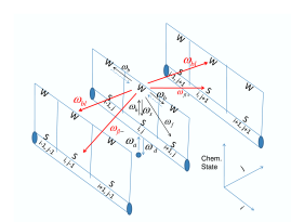
Figure 1: (Color online) A schematic representation of our model, together will the allowed transitions and the corresponding rate constants.

The equispaced binding sites for KIF1A on a given protofilament of the MT are labelled by the integer index $i$ ($i=1,...,L$). We use the integer index $j$ to label the protofilaments; the position of each binding site is denoted completely by the pair $(i,j)$. Because of the tubular geometry of the MT, periodic boundary conditions along the $j$-direction would be a natural choice. We impose periodic boundary conditions also along the $i$-direction, as it not only simplifies our analytical calculations but is also adequate to answer the fundamental questions which we address in this communication.

In each mechano-chemical cycle a KIF1A motor hydrolyzes one molecule of adenosine triphosphate (ATP) which supplies the mechanical energy required for its movement. The experimental results on KIF1A motors okada1 ; okada4 ; okada5 indicate that a simplified description of its mechano-chemical cycle in terms of a 2-state model nosc would be sufficient to understand their traffic on a MT. In the two “chemical” states labelled by the symbols $S$ and $W$ the motor is, respectively, strongly and weakly bound to the MT.

In the NOSC model, a KIF1A molecule is allowed to attach to (and detach from) a site with rates $\omega_{a}$ (and $\omega_{d}$). The rate constant $\omega_{b}$ corresponds to the unbiased Brownian motion of the motor in the state $W$. The rate constant $\omega_{h}$ is associated with the process driven by ATP hydrolysis which causes the transition of the motor from the state $S$ to the state $W$. The rate constants $\omega_{f}$ and $\omega_{s}$, together, capture the Brownian ratchet mechanism julicher ; reimann of a KIF1A motor. Moreover, any movement of the motor under these rules is, finally, implemented only if the target site is not already occupied by another motor.

The rules of time evolution in the extended NOSC model proposed here are identical to those in the NOSC model, except for the following additional lane-changing rules (see fig.1):
a motor weakly-bound (i.e., in state $W$) to the binding site $i$ on the protofilament $j$ is allowed to move to the positions $(i,j+1)$ and $(i,j-1)$
(i) without simultaneous change in its chemical state, both the corresponding rates being $\omega_{bl}$;
(ii) with simultaneous transition to the chemical state $S$, the corresponding rate constants being $\omega_{fl+}$ and $\omega_{fl-}$, respectively.

Let $S_{i}(j,t)$ and $W_{i}(j,t)$ denote the probabilities for a motor to be in the “chemical” states $S$ and $W$, respectively, at site $i$ on the protofilament $j$. In the extended NOSC model, under mean-field approximation, the master equations for the probabilities $S_{i}(j,t)$ and $W_{i}(j,t)$ are given by

$$\frac{dS_{i}(j,t)}{dt} = \omega_{a}[1-S_{i}(j,t)-W_{i}(j,t)]-\omega_{h}S_{i}(j,t)-\omega_{d}S_{i}(j,t)+\omega_{s}W_{i}(j,t)+\omega_{f}W_{i-1}(j,t)[1-S_{i}(j,t)-W_{i}(j,t)]$$ (1)

$$+\omega_{fl+}[W_{i}(j-1,t)][1-S_{i}(j)-W_{i}(j)]+\omega_{fl-}[W_{i}(j+1,t)][1-S_{i}(j)-W_{i}(j)],$$

$$\frac{dW_{i}(j,t)}{dt} = \omega_{h}S_{i}(j,t)-\omega_{s}W_{i}(j,t)-\omega_{f}W_{i}(j,t)[1-S_{i+1}(j,t)-W_{i+1}(j,t)]$$ (2)

$$-\omega_{b}W_{i}(j,t)[2-S_{i+1}(j,t)-W_{i+1}(j,t)-S_{i-1}(j,t)-W_{i-1}(j,t)]$$

$$+\omega_{b}[W_{i-1}(j,t)+W_{i+1}(j,t)][1-S_{i}(j,t)-W_{i}(j,t)]$$

$$+\omega_{bl}[W_{i}(j-1,t)+W_{i}(j+1,t)][1-S_{i}(j,t)-W_{i}(j,t)]$$

$$-\omega_{bl}W_{i}(j,t)[2-S_{i}(j+1,t)-W_{i}(j+1,t)-S_{i}(j-1,t)-W_{i}(j-1,t)]$$

$$-\omega_{fl+}W_{i}(j,t)[1-S_{i}(j+1,t)-W_{i}(j+1,t)]-\omega_{fl-}W_{i}(j,t)[1-S_{i}(j-1,t)-W_{i}(j-1,t)].$$

Rate constant	numerical value/range (s-1)
$\omega_{a}$	0.1 - 10.0
$\omega_{d}$	0.1
$\omega_{h}$	0 - 250
$\omega_{s}$	145
$\omega_{f}$	55

Table 1: Rate constants of the NOSC model which have been extracted from empirical data on single KIF1A experiments greulich .

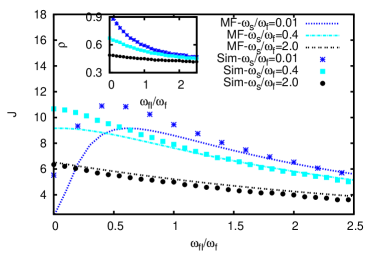
Figure 2: (Color online) Flux per lane (and, in the inset, average density of the motors on each lane) are plotted against $\omega_{fl}/\omega_{f}$ for a few values of $\omega_{s}/\omega_{f}$. Our mean-field predictions (labelled MF) are plotted by lines while the discrete data points (labelled Sim) have been obtained from our computer simulations of the model.

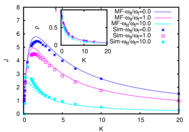
Figure 3: (Color online) Same as in Fig.2, except that the data are plotted against $K$ for a few values of $\omega_{fl}/\omega_{f}$.

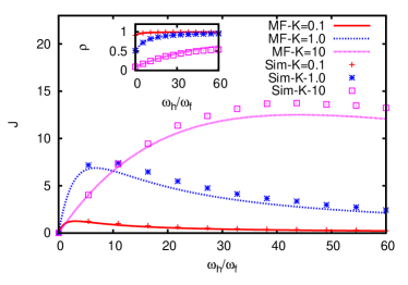
Figure 4: (Color online) Same as in Fig.2, except that the data are plotted against $\omega_{h}/\omega_{f}$ for a few values of $K$.

In the steady state under periodic boundary conditions, ${\tilde{S}}=S_{i}(j,t)$ and ${\tilde{W}}=W_{i}(j,t)$, independent of $t$ and irrespective of $i$ and $j$; from eqs.(1) and (2), we get

$${\tilde{S}}=\frac{-{\tilde{\Omega_{h}}}-{\tilde{\Omega_{s}}}-({\tilde{\Omega_{s}}}-1)K+{\sqrt{{\tilde{D}}}}}{2K(1+K)}$$ (3)

$${\tilde{W}}=\frac{{\tilde{\Omega_{h}}}+{\tilde{\Omega_{s}}}+({\tilde{\Omega_{s}}}+1)K-{\sqrt{{\tilde{D}}}}}{2K},$$ (4)

where $K=\omega_{d}/\omega_{a}$, ${\tilde{\Omega_{h}}}=\omega_{h}/{\tilde{\omega_{f}}}$, ${\tilde{\Omega_{s}}}=\omega_{s}/{\tilde{\omega_{f}}}$, with ${\tilde{\omega_{f}}}=\omega_{f}+\omega_{fl+}+\omega_{fl-}$, and

$${\tilde{D}}=4{\tilde{\Omega_{s}}}K(1+K)+({\tilde{\Omega_{h}}}+{\tilde{\Omega_{s}}}+({\tilde{\Omega_{s}}}-1)K)^{2}.$$ (5)

The average total density of the motors attached to each filament of the MT in the steady state is given by

$$\rho={\tilde{S}}+{\tilde{W}}=\frac{{\tilde{\Omega_{h}}}+{\tilde{\Omega_{s}}}+({\tilde{\Omega_{s}}}+1)K-\sqrt{{\tilde{D}}}+2}{2(1+K)}.$$ (6)

Using the expressions (3) and (4) for ${\tilde{S}}$ and ${\tilde{W}}$, respectively, in the expression

$$J=\omega_{f}{\tilde{W}}(1-{\tilde{S}}-{\tilde{W}})$$ (7)

for the flux of KIF1A motors per lane of the MT highway, we get

$$J=\frac{\omega_{f}\biggl{[}K^{2}-\biggl{(}{\tilde{\Omega_{h}}}+(1+K){\tilde{\Omega_{s}}}-\sqrt{{\tilde{D}}}\biggr{)}^{2}\biggr{]}}{4K(1+K)}.$$ (8)

For graphical presentation of our main results, we use the estimates of the rate constants, listed in table 1, which were extracted earlier greulich from empirical data on single KIF1A (we use $\omega_{h}=125$ s^-1). Since no estimate of $\omega_{fl+}$ and $\omega_{fl-}$ are available, we use $\omega_{fl+}=\omega_{fl-}=\omega_{fl}$ and vary the single parameter $\omega_{fl}/\omega_{f}$ over a wide range to explore the consequences of different rates of lane changing. The flux per lane (obtained from (8)) and the average density $\rho$ (given by (6)) are plotted against $\omega_{fl}/\omega_{f}$ in Fig. 2 for several different values of $\omega_{s}/\omega_{f}$ and compared with the corresponding simulation data.

Recall that flux is essentially an average of the product of the density and speed of the motors. For sufficiently high $\omega_{s}/\omega_{f}$, the density $\rho$ is small even in the absence of lane changing ($\omega_{fl}=0$) and, consequently, the motors feel hardly any steric hindrance; increasing $\omega_{fl}/\omega_{f}$ in this regime of $\omega_{s}/\omega_{f}$ has very little effect on the average speed of the motors and it is the decreasing density that is responsible for the monotonic decrease of $J$ with $\omega_{fl}$.

In sharp contrast, at sufficiently low values of $\omega_{s}/\omega_{f}$, $J$ varies non-monotonically with $\omega_{fl}/\omega_{f}$. In this regime of $\omega_{s}/\omega_{f}$, at $\omega_{fl}=0$, the high density of $\rho$ causes steric hindrances which, in turn, leads to small $J$. When $\omega_{fl}$ is “switched on”, $\rho$ decreases with increasing $\omega_{fl}$ and $J$ increases up to a maximum because of the weakening of the hindrance effects. But, beyond a certain range of $\omega_{fl}/\omega_{f}$, the density of motors becomes so low that the movement of the motors is practically free of mutual hindrance; the decrease of $J$ beyond its maximum is caused by the further reduction of density. Larger difference between the predictions of our approximate analytical calculations and computer simulation data at lower values of $\omega_{s}/\omega_{f}$ arises from the fact that the mean-field approximation neglects correlations which increases with increasing densitity of the motors.

The above interpretation of trends of variations of $J$ in Fig. 2 in terms of the corresponding variation of $\rho$ is consistent with the results shown in Figs. 3 and 4. But, why does $\rho$ decrease monotonically with increasing $\omega_{fl}/\omega_{f}$? Increasing $\omega_{fl}$, keeping all the other rate constants unaltered, leads to higher overall rate of transitions into strongly-bound states. Since, detachments of the motors from the microtubule track take place from the strongly bound state (see footnote note ), the steady-state density is lower for higher values of $\omega_{fl}/\omega_{f}$.

An approximate expression for $J$, which is obtained by retaining only the terms upto the first order in $\omega_{fl}$ in a Taylor expansion of the right hand side of (8), is given by

$$J=J_{0}-4\biggl{(}\frac{\omega_{fl}}{\omega_{f}}\biggr{)}J_{0}+\biggl{(}\frac{\omega_{fl}}{2\sqrt{D}(1+K)}\biggr{)}\biggl{(}[(1+K)\Omega_{s}+K]^{2}+[(1+K)\Omega_{s}-\sqrt{D}]^{2}-[\Omega_{h}-\sqrt{D}]^{2}-[\Omega_{h}-K]^{2}\biggr{)}+O(\omega_{fl}^{2})$$ (9)

where $J_{0}$ is the flux corresponding to $\omega_{fl}=0$ (i.e., in the absence of lane changing). The approximate formula (9) still provides a reasonably good estimate of the flux even when $\omega_{fl}$ is as large as $\omega_{f}$.

In this communication we have extended the NOSC model for KIF1A traffic on MT nosc ; greulich by incorporating processes which correspond to shifting of the motors from one protofilament to another. These processes are analogous to lane changing of vehicles on multi-lane highways. On the basis of analytical treatment and computer simulations of the extended NOSC model, we have predicted the effects of such lane-changing on $J$, the steady-state flux of the KIF1A motors per lane. Over a wide region of parameter space, $J$ decreases monotonically with increasing value of $\omega_{fl}$, a rate constant for lane-changing. However, in some regions of parameter space, $J$ varies non-monotonically with increasing $\omega_{fl}$. We have interpreted the results by correlating the observed trends of variation of $J$ with the corresponding variation of $\rho$, the average density of motors on a lane, and establishing the dependence of $\rho$ on $\omega_{fl}$.

Double-headed conventional kinesin rarely changes lane ray93 . Double-headed dyneins may change lane in-vitro wang95 ; peterson06 but, perhaps, not in-vivo watanabe07 . The bound head of a double-headed motor imposes constraints on the stepping of the unbound head. Since such constraints do not exist for single-headed kinesins, KIF1A may find it easier to change lane. However, KIF1A may dimerize in-vivo tomishige . Therefore, in-vitro experiments with fluorescently labelled KIF1A would be able to test our theoretical predictions. In particular, variations of $J$ with $K$ and $\omega_{h}$ (see figs.3 and 4) can be probed by varying concentration of KIF1A and ATP molecules, respectively, in the solution.

Acknowledgements: We thank J. Howard, R. Mallik, A. Schadschneider and G.Schütz for useful suggestions. This work is supported by the NUS-India Research Initiatives, a Faculty Research Grant (NUS), a CSIR research grant (India), physics department of NUS and NUS-IITK MoU.

References

- (1) M. Schliwa, (ed.) Molecular Motors, (Wiley-VCH, 2003).
- (2) J. Howard, Mechanics of motor proteins and the cytoskeleton, (Sinauer Associates, 2001).
- (3) D. Chowdhury, L. Santen, and A. Schadschneider, Phys. Rep. 329, 199 (2000).
- (4) D. Chowdhury, A. Schadschneider and K. Nishinari, Phys. of Life Rev. 2, 318 (2005).
- (5) R. Lipowsky, S. Klumpp, and T. M. Nieuwenhuizen, Phys. Rev. Lett. 87, 108101 (2001); R. Lipowsky et al., Physica A 372, 34 (2006) and references therein.
- (6) A. Parmeggiani, T. Franosch and E. Frey, Phys. Rev. Lett. 90, 086601 (2003); Phys. Rev. E 70, 046101 (2004).
- (7) M.R. Evans, R. Juhasz and L. Santen, Phys. Rev. E 68, 026117 (2003).
- (8) V. Popkov et al., Phys. Rev. E 67, 066117 (2003).
- (9) B. Schmittmann and R.K.P. Zia, in: Phase Transition and Critical Phenomena, Vol. 17, eds. C. Domb and J. L. Lebowitz (Academic Press, 1995).
- (10) B. Derrida, Phys. Rep. 301, 65 (1998)
- (11) G. M. Schütz, Phase Transitions and Critical Phenomena, vol. 19 (Acad. Press, 2001).
- (12) E. Pronina and A.B. Kolomeisky, J. Phys. A 37, 9907 (2004); Physica A 372, 12 (2006).
- (13) T. Mitsudo and H. Hayakawa, J. Phys. A 38, 3087 (2005).
- (14) R. Wang et al., arXiv:q-bio/0703043v1 (2007).
- (15) T. Reichenbach, T. Franosch and E. Frey, Phys. Rev. Lett. 97, 050603 (2006); T. Reichenbach, E. Frey and T. Franosch, New J. Phys. 9, 159 (2007).
- (16) K. Nishinari et al., Phys. Rev. Lett. 95, 118101 (2005)
- (17) P. Greulich et al., Phys. Rev. E 75, 041905 (2007).
- (18) Y. Okada and N. Hirokawa, Science 283, 1152 (1999); PNAS 97, 640 (2000).
- (19) Y. Okada, H. Higuchi and N. Hirokawa, Nature, 424, 574 (2003).
- (20) R. Nitta et al., Science 305, 678 (2004).
- (21) F. Jülicher, A. Ajdari and J. Prost, Rev. Mod. Phys. 69, 1269 (1997).
- (22) P. Reimann, Phys. Rep. 361, 57 (2002).
- (23) The terminology “strongly-bound ” and “weakly-bound” states, still used for historical reasons, is misleading; actually, the active detachment of KIF1A from the MT track takes place while in a transient intermediate state during the transition from the “strongly-bound ” state to the “weakly-bound” state okada5 .
- (24) S. Ray, et al., J. Cell Biol. 121, 1083 (1993).
- (25) Z. Wang, S. Khan and M.P. Sheetz, Biophys. J. 69, 2011 (1995).
- (26) S.L. Reck-Peterson et al., Cell 126, 335 (2006).
- (27) T. Watanabe et al., BBRC 359, 1 (2007).
- (28) M. Tomishige, D.R. Klopfenstein and R.D. Vale, Science 297, 2263 (2002).