Non Perturbative Renormalization Group and Bose-Einstein Condensation

1 Introduction

These lectures are centered around a specific problem, the effect of weak repulsive interactions on the transition temperature $T_{c}$ of a Bose gas. This problem provides indeed a beautiful illustration of many of the techniques which have been discussed at this school on effective theories and renormalization group. Effective theories are used first in order to obtain a simple hamiltonian describing the atomic interactions: because the typical atomic interaction potentials are short range, and the systems that we consider are dilute, these potentials can be replaced by a contact interaction whose strength is determined by the $s$-wave scattering length. Effective theories are used next in order to obtain a simple formula for the shift in $T_{c}$: one exploits there the fact that near $T_{c}$ the physics is dominated by low momentum modes whose dynamics is most economically described in terms of classical fields; the ingredients needed to calculate the shift of $T_{c}$ can be obtained from this classical field theory. Finally the renormalization group is used both to obtain a qualitative understanding, and also as a non perturbative tool to evaluate quantitatively the shift in $T_{c}$.

In the first lecture, I recall some known aspects of Bose-Einstein condensation of the ideal gas. Then I turn to an elementary discussion of the interaction effects, and introduce an effective theory with a contact interaction tuned to reproduce the scattering length of the atom-atom interaction. I show that at the mean field level, weak repulsive interactions produce no shift in $T_{c}$. Finally, I briefly explain why approaching the transition from the low temperature phase is delicate and may lead to erroneous conclusions.

In the second lecture I establish the general formula for the shift of $T_{c}$:

$${\Delta T_{c}\over T_{c}^{0}}={T_{c}-T_{c}^{0}\over T_{c}^{0}}=c(an^{1/3}),$$ (1)

where $a$ is the s-wave scattering length for the atom-atom interaction, and $T_{c}^{0}$ the transition temperature of the ideal gas at density $n$. This formula holds in leading order in the parameter $an^{1/3}$ which measures the diluteness of the system. Getting formula (1) involves a number of steps. First I explain why perturbation theory cannot be used to calculate $\Delta T_{c}$, however small $a$ is. Then I show that the problem with the perturbative expansion is localized in a particular subset of Feynman diagrams that are conveniently resummed by an effective theory of a classical 3-dimensional field. The outcome of the analysis is the formula (1) where $c$ is given by the following integral

$$c\propto\int{d^{3}p\over(2\pi)^{3}}\left({1\over p^{2}+\Sigma(p)}-{1\over p^{2}}\right).$$ (2)

where the proportionality coefficient, not written here, is a known numerical factor, and $\Sigma$ is the self-energy of the classical field, whose calculation requires non perturbative techniques.

In the last lecture, I use the non perturbative renormalization group (NPRG) in order to estimate $c$. This requires the knowledge of the 2-point function of the effective 3-dimensional field theory for all momenta, and in particular in the cross-over between the critical region of low momenta and perturbative region of high momenta. This cross-over region is where the dominant contribution to the integral (2) comes from. In order to obtain an accurate determination of $\Sigma(p)$, it has been necessary to develop new techniques to solve the NPRG equations. Describing those techniques in detail would take us too far. I shall only present in this lecture the material that can help the student not familiar with the NPRG to understand how it works, and how it can be used. I shall do so by discussing several simple cases that at the same time provide indications on the approximation scheme that has been developed in order to calculate $\Sigma(p)$. I shall end by reporting and discussing the results obtained with the NPRG, and compare them to those obtained using other non perturbative techniques.

Recent discussion of Bose-Einstein condensation can be found in Pitaevskii03 ; Pethick02 ; RMP ; Leggett:2001 ; Andersen:2003qj . The equation (1) for the shift of $T_{c}$ is derived and discussed in the series of papers 3/2club ; BigN ; bigbec ; NEW ; Fuchs04 . Much of the material of the last lecture is borrowed from the papers Blaizot:2004qa ; Blaizot:2005wd ; Blaizot:2006vr ; Blaizot:2005xy ; Blaizot:2006ak .

2 LECTURE 1. Bose-Einstein condensation

2.1 Bose-Einstein condensation for the non interacting gas

• The discussion of Bose-Einstein condensation of the ideal Bose gas in the grand canonical ensemble is standard. We consider a homogeneous system of identical spinless bosons of mass $m$, at temperature $T$ . The occupation factor of a single particle state with momentum ${\bf p}$ is

  $$n_{\bf p}={1\over{\rm e}^{(\varepsilon^{0}_{\bf p}-\mu)/T}-1},\qquad\varepsilon^{0}_{\bf p}={p^{2}\over 2m},$$ (3)

  where $\mu$ is the chemical potential. The number density of non-condensed particles is given by

  $$n=\int{d^{3}{\bf p}\over(2\pi)^{3}}\,n_{\bf p}\equiv n(\mu,T).$$ (4)

  For small density, the chemical potential is negative and large in absolute value, ${\rm e}^{-\mu/T}\gg 1$. The gas is then described by Boltzmann statistics:

  $$n_{\bf p}\approx{\rm e}^{-(\varepsilon^{0}_{\bf p}-\mu)/T},\qquad n\approx{\rm e}^{\mu/T}\lambda^{-3},$$ (5)

  where $\lambda$ is the thermal wavelength:

  $$\lambda=\sqrt{{2\pi\over mT}}.$$ (6)

  Unless specified otherwise, we use units such that $\hbar=1,k_{B}=1$. Boltzmann’s statistics applies as long as $n\lambda^{3}\ll 1$, that is, as long as the thermal wavelength is small compared to the interparticle distance. As one lowers the temperature, keeping the density fixed, the chemical potential increases, and so does the thermal wavelength. Eventually, as $\mu\to 0_{-}$, the density of non condensed particles reaches a maximum

  $$n=\int{d^{3}p\over(2\pi)^{3}}{1\over{\rm e}^{\varepsilon^{0}_{\bf p}/T}-1}=n(\mu=0,T)={\zeta(3/2)\over\lambda^{3}},$$ (7)

  where $\zeta(z)$ is the Riemann zeta-function and $\lambda$ the thermal wavelength. As one keeps lowering the temperature, particles start to accumulate in the lowest energy single particle state. This is the onset of Bose-Eisntein condensation, which takes place then when

  $$n\lambda^{3}=\zeta(3/2)\approx 2.612.$$ (8)

  At this point the thermal wavelength has become comparable to the interparticle spacing. Eq. (8) defines the critical line in the $n,T$ plane (see Fig. 1). In particular, the critical temperature is given by

  $$T_{c}^{0}={2\pi\over m}\left({n\over\zeta(3/2)}\right)^{2/3}.$$ (9)

  It is a function only of the mass of the atom, and of the density.

  

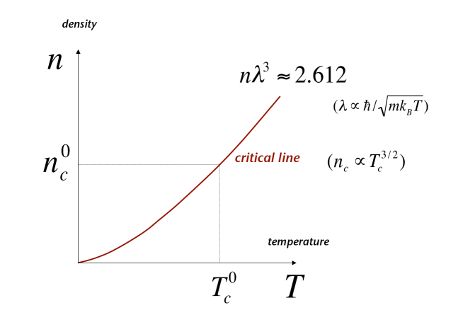
  Figure 1: Critical line in the $(\mu,T)$ plane for the ideal Bose gas

  For $T<T_{c}^{0}$, the chemical potential stays equal to zero and the single particle state ${\bf p}=0$ is macroscopically occupied, with density $n_{0}\propto n$ given by

  $$n_{0}(T)=n\left(1-\left({T\over T_{c}^{0}}\right)^{3/2}\right).$$ (10)

• The occurrence of condensation relies on the existence of a maximum of the integral (4) fixing the number of non condensed atoms. This depends on the number of spatial dimensions. In 2 dimensions, the integral diverges logarithmically as $\mu\to 0_{-}$:

  $$n\lambda^{2}=-\ln\left(1-{\rm e}^{\mu/T}\right).$$ (11)

  In this case, there is no limit to the number of thermal particles, hence no condensation in the lowest energy mode.

• The Bose-Einstein condensation of the non-interacting gas has some pathological features. In particular the compressibility

  $${1\over n^{2}}{\partial n\over\partial\mu}={1\over n^{2}}{1\over T}\int{d^{3}p\over(2\pi)^{3}}n_{\bf p}(1+n_{\bf p}),$$ (12)

  diverges when $\mu\to 0_{-}$. Also the fluctutation of the number of particles in the condensate,

  $$\sqrt{\Delta\langle N^{2}\rangle}=\sqrt{N_{0}(N_{0}+1)}\simeq N_{0},$$ (13)

  is of the same order of magnitude as the average value $N_{0}$. Such features can be related to the large degeneracy of states in Fock space that appears as $\mu\to 0$.

  Consider indeed the ground state in Fock space of the hamiltonian of the non interacting Bose gas,

  $$H_{0}-\mu N=\sum_{\bf p}\left(\varepsilon^{0}_{\bf p}-\mu\right)a^{\dagger}_{\bf p}a_{\bf p}.$$ (14)

  If $\mu<0$, then the ground state is the vacuum, with no particle present in the system: adding a particle costs a positive “free-energy” $-\mu$. When $\mu=0$, there appears a huge degeneracy in Fock space: all the states with an arbitrary number of particles in the single particle state ${\bf p}=0$ are degenerate. If $\mu>0$, then there is no minimum, the more particle one adds in the state ${\bf p}=0$, the more free energy one gains ($-\mu$ for each added particle). Note that here the chemical potential does not fully plays its role of controlling the density: either it is negative, and the density is zero, or it is positive and the density is infinite; if it vanishes the density is arbitrary.

  To relate the large degeneracy to the large fluctuations (13), one may use a simple maximum entropy technique to determine the most likely state with $N_{0}$ particles in the degenerate space. This calculation parallels the corresponding calculation done in the grand canonical ensemble at finite temperature. Maximizing

  $$\hat{S}=-\sum_{n}p_{n}\ln p_{n}+\mu\sum_{n}np_{n}-\lambda\sum_{n}p_{n},$$ (15)

  with the constraints

  $$\sum_{n}p_{n}=1,\qquad\sum_{n}np_{n}=N_{0},$$ (16)

  one finds

  $$p_{n}={1\over Z}{\rm e}^{\mu n},\qquad Z={1\over 1-{\rm e}^{\mu}},\qquad\mu=-\ln\left(1+{1\over N_{0}}\right).$$ (17)

  For large $N_{0}$,

  $$p_{n}\approx{{\rm e}^{-n/N_{0}}\over N_{0}},$$ (18)

  which leads indeed to the large fluctuations (13).

  Of course, some of the pathologies of the ideal Bose gas in the grand canonical ensemble could be eliminated by working in the canonical ensemble, where the particle number is fixed (see e.g. Ziff77 ). However, we shall keep the discussion within the grand canonical ensemble, as it is closer to familiar field theoretical techniques. This allows us in particular to treat Bose-Eisntein condensation (of the interacting gas) as a symmetry breaking phenomenon.

  The large degeneracy of states in Fock space implies that infinitesimal interactions could have a large effect, and indeed they do: as soon as weak repulsive interactions are present the large fluctuations are damped, and the compressibility becomes finite .

2.2 Interactions in the dilute gas

• As we shall discuss later in this lecture, the dominant effect of the interactions in the dilute gas can be accounted for by an effective contact interaction whose strength $g$ is proportional to the $s$-wave scattering length $a$:

  $$V({\bf r_{1}-r_{2}})=g\delta({\bf r_{1}-r_{2}}),\qquad g={4\pi a\over m}.$$ (19)

• In the mean field (Hartree-Fock) approximation, which is also the leading order in $a$, the effect of the interaction is a simple shift of the single particle energies:

  $$\varepsilon_{\bf p}^{0}\longrightarrow\varepsilon_{\bf p}^{0}+2gn,$$ (20)

  where the factor 2 comes from the exchange term.

  It is easy to see that this produces no shift in $T_{c}$: because the shift of the single particle energy is constant, independent of the momentum, eq. (4) which gives the number density of non condensed particles, can be written

  $$n=n(\mu-\Delta\mu,T)$$ (21)

  with

  $$\Delta\mu=2gn.$$ (22)

  Bose-Einstein condensation now occurs when $\mu-\Delta\mu=0$, instead of $\mu=0$ in the non interacting case, but clearly the critical line is identical to that given by eq. (8).

  Of course, because the Hartree-Fock self-energy in eq. (20) depends on the density, the relation between the chemical potential at the transition and the critical density is more complicated than in the non-interacting case. The transition now takes place at a finite value of the chemical potential, and some of the pathologies of the ideal gas disappear. In particular the compressibility remains finite at $T_{c}$ (fluctuations remain important though):

  $${\partial n\over\partial\mu}={{1\over T}\int_{p}n_{p}(1+n_{p})\over 1+{2g\over T}\int_{p}n_{p}(1+n_{p})}\simeq{1\over 2g}.$$ (23)

• The presence of the interactions allows us to treat the phenomenon of Bose Einstein condensation as a symmetry breaking phenomenon. Let us return first to the ground state, and calculate the free energy

  $${\Omega(n_{0})\over{\cal V}}=-\mu n_{0}+{g\over 2}n_{0}^{2},$$ (24)

  where ${\cal V}$ is the volume. $\Omega(n_{0})$ is the expectation value of the hamiltonian (14) to which is added the interaction (19), $V\sim(g/2)a^{\dagger}_{0}a^{\dagger}_{0}a_{0}a_{0}$, in a coherent state containing an average number of particles $N_{0}=n_{0}{\cal V}$ in the state ${\bf p=0}$, $|n_{0}\rangle\sim\exp{\sqrt{N_{0}}a^{\dagger}_{0}}|0\rangle$. In contrast to what happened for the ideal gas, it is now possible to minimize $\Omega(n_{0})$ w.r.t. $n_{0}$ in order to find the optimum ground state for a given $\mu$. One gets

  $$n_{0}=\mu/g.$$ (25)

  Thus the ground state has now a finite number of particles, and the fluctuations are normal, proportional to the square root of the mean value. The density in the ground state is $n=\partial\Omega/\partial\mu=n_{0}$, and the pressure is $P=-\Omega(n_{0}=\mu/g)/{\cal V}=gn^{2}/2$, so that also at zero temperature the compressibility is finite, $\chi^{-1}=ndP/dn=gn^{2}$. Note however that the coherent state is a state with a non definite number of particles: the symmetry related to particle number conservation is spontaneously broken. We shall return later to the similar picture at finite temperature, and come back to this issue of symmetry breaking.

2.3 Atoms in a trap

Although our main discussion concerns homogeneous systems, it is instructive to contrast the situation in homogeneous systems to what happens in a trap. We shall consider here a spherical harmonic trap, corresponding to the following external potential

$$V(r)={1\over 2}m\omega_{0}^{2}r^{2}.$$ (26)

• Consider first the non interacting gas. We assume the validity of a semiclassical approximation allowing us to express the particle density as the following phase space integral:

  $$n(r)=\int{d^{3}p\over(2\pi)^{3}}{1\over{\rm e}^{(\varepsilon(r,p)-\mu)/T}-1},$$ (27)

  where $\varepsilon(r,p)=p^{2}/2m+(1/2)m\omega_{0}^{2}r^{2}$. This requires that the temperature is large compared to the level spacing, $k_{B}T\gg\hbar\omega_{0}$, a condition well satisfied near the transition if $N$, the number of particles in the trap, is large enough. The number density in the trap can be written as

  $$N=\int d^{3}{\bf r}\,n(\mu-{1\over 2}m\omega_{0}^{2}r^{2},T),$$ (28)

  where $n(\mu,T)$ is the function (4). Thus in a wide trap for which the semiclassical approximation is valid, the particles experience the same conditions as in a uniform system with a local effective chemical potential $\mu-{1\over 2}m\omega_{0}^{2}r^{2}$. In particular, eq. (27) shows that the density at the center of the trap is related to the chemical potential $\mu$ by the same relation as in the homogeneous gas. It follows that $T_{c}^{0}$ is determined by the same condition as for the homogeneous gas, that is, $n(0)\lambda^{3}=2.612$ where $n(0)$ is the density at the center of the trap. An explicit calculation gives

  $${k_{B}T_{c}^{0}\over\hbar\omega_{0}}=\left({N\over\zeta(3)}\right)^{1/3},$$ (29)

  with $\zeta(3)=1.202$. Note that while the condensation condition is “universal” when expressed in terms of the density at the center of the trap, the dependence of $T_{c}^{0}$ on $N$ depends on the form of the confining potential. In the present case, the $N$ dependence can be obtained from the following heuristic argument. For a temperature $T\mathrel{\hbox to0.0pt{\raise 2.20013pt\hbox{$>$}\hss}{\lower 2.20013pt\hbox{$\sim$}}}T_{c}^{0}$ the particle density is approximately given by the classical formula

  $$n\sim{\rm e}^{-{m\omega_{0}^{2}r^{2}}/{2T}},$$ (30)

  so that the thermal particles occupy a cloud of radius $R_{th}\sim\sqrt{T/m\omega_{0}^{2}}\sim a^{2}_{ho}/\lambda$, where $\alpha_{ho}=1/\sqrt{m\omega_{0}}$ is the characteristic radius of the harmonic trap and $\lambda\sim 1/\sqrt{mT}$ is the thermal wavelength. The average density in the thermal cloud is $\bar{n}\sim NR_{th}^{-3}$. At the transition, the interparticle distance is of the order of the thermal wavelength, so that, $\bar{n}^{1/3}\sim N^{1/3}\lambda/a^{2}_{ho}\sim\lambda^{-1}$, or $N^{1/3}\lambda^{2}\sim a^{2}_{ho}$, from which the relation $T_{c}^{0}\sim\omega N^{1/3}$ follows.

  Note that the confining potential makes condensation easier than in the uniform case. This is related to the fact that the density of single particle states in a trap decreases more rapidly with decreasing energy than in a uniform system: it goes as $\varepsilon^{d-1}$ in a trap and as $\varepsilon^{d/2-1}$ in a uniform system, where $d$ is the number of spatial dimensions. It follows in particular that, in a trap, condensation can occur in $d=2$, in contrast to the homogeneous case; the heuristic argument presented above yields then $T_{c}^{0}\sim\omega N^{1/2}$. Note however that the effects of the interactions in a 2-dimensional trap are subtle (for a recent discussion see PNAS ).

• The leading effect of repulsive interactions in a trap is to push the particles away from the center of the trap, thereby decreasing the central density. This effect is analogous to that produced by an increase of the temperature. One expects therefore the interactions to lead to a decrease of the transition temperature. To estimate this, we note that, in the presence of interactions, the density is still given by eq. (30) after substituting $(1/2)m\omega_{0}^{2}r^{2}\to(1/2)m\omega_{0}^{2}r^{2}+2gn(r).$ A simple calculation gives then the density $n(r)$ (for $r$ not too large, and to leading order in $a$) in terms of the density $n(0)$ at the center of the trap Fuchs04 :

  $$n({\bf r}) \approx n(0){\rm e}^{-\beta(m\omega_{0}^{2}r^{2}/2)(1-2gn(0)/T)}$$ (31)

  $$\approx n(0)\left[1-{1\over 2T}{m\omega_{0}^{2}r^{2}\over 1+4a\lambda^{2}n(0)}\right].$$

  This result suggests that the effect of the interaction can also be viewed as a modification of the oscillator frequency, $\omega_{0}^{2}\to\omega_{0}^{2}/(1+4a\lambda^{2}n(0)$. This is enough to estimate the shift in $T_{c}$:

  $${\Delta T_{c}\over T_{c}^{0}}={\Delta\omega\over\omega_{0}}\sim-a\lambda^{2}n(0)\sim-{a\over a_{ho}}N^{1/6},$$ (32)

  where, in the last step, we have used the fact that $n(0)\sim\lambda^{-3}$ at the transition. A more explicit calculation yields the proportionality coefficient $-1.32$ Giorgini96 .

  It is important to keep in mind that this effect of mean field interactions on $T_{c}$ is very different from the one that leads to eq. (1) (indeed the sign of the effect is different). If we were comparing systems at fixed central density rather than at fixed particle number, there would be no shift of $T_{c}$ (see the discussion in Fuchs04 ).

2.4 The two-body problem

We now come back to the construction of the effective interaction that can be used in many-body calculations of the dilute gas. We shall in particular recall how effective field theory can be used to relate the effective interaction to the low energy scattering data. More on the use of effective theories can be found in the lecture by T. Schäfer in this volume Schafer:2006yf . A pedagogical introduction is given in Ref. Kaplan:2005es .

Consider two atoms of mass $m$ interacting with the central two-body potential $V(r)$, with ${\bf r}$ the relative coordinate and $r=|{\bf r}|$. The relative wave function satisfies the Schrödinger equation

$$\left[-{\hbar^{2}\,\nabla^{2}\over m}+V(r)\right]\psi({\bf r})=E\psi({\bf r}).$$ (33)

The scattering wave function is given by ($E=\hbar^{2}k^{2}/m$)

$$\psi_{\bf k}({\bf r})={\rm e}^{i{\bf k}\cdot{\bf r}}+f({\bf k}^{\prime},{\bf k}){{\rm e}^{ikr}\over r},$$ (34)

where ${\bf k}$ is the initial relative momentum (with $k=|{\bf k}|$), while ${\bf k}^{\prime}$ is the final relative momentum. The scattering is elastic and because the potential is rotationally invariant, the scattering amplitude $f({\bf k}^{\prime},{\bf k})$ is a function only of the scattering angle $\theta$ in the center of mass frame, and of the energy $E=\hbar^{2}k^{2}/m$. For short-range interactions, the interaction takes place predominantly in the $s$-wave, and the scattering amplitude becomes of a function of the energy only. It has then the following low momentum expansion:

$$f(E)={1\over-{1\over a}+{r_{0}\over 2}k^{2}-ik}\qquad\hbar k=\sqrt{mE}.$$ (35)

where $a$ is the scattering length, $r_{0}$ the effective range, and the neglected terms in the denominator involve higher powers of $k$. In the very low momentum limit, when $kr_{0}\,ka\ll 1$, one can ignore the effective range. Then the scattering amplitude depends on a single parameter, $a$.

The scattering amplitude can be expressed as the matrtix element between plane wave states of the T-matrix:

$$\langle{\bf k^{\prime}}|T|{\bf k}\rangle=-{4\pi\hbar^{2}\over m}f({\bf k^{\prime},k}),$$ (36)

and the T-matrix itself can be calculated in terms of the Green function $G_{0}$

$$T=V-VG_{0}T,$$ (37)

where

$$G_{0}(E)={1\over H_{0}-E},$$ (38)

and $E\to E+i\eta$ with $E$ real for the retarded Green’s function $G_{0}^{R}$. The following formal relations are useful

$$H=H_{0}+V,\qquad G^{-1}=H-E=G_{0}^{-1}+V,$$ (39)

and

$$T=V-VGV=V-VG_{0}T\qquad T^{-1}=V^{-1}+G_{0}.$$ (40)

Note that both $G(E)$ and $T(E)$ are analytic functions of $E$, with poles on the negative real axis corresponding to the energies of the bound states, and a cut on the real positive axis.

Let us now turn to the many-body problem. Assuming that the atoms interact only through the two body potential $V(r)$, we can write the interaction hamiltonian as

$$V={1\over 2}\int d^{3}{\bf r_{1}}{\rm d}^{3}{\bf r_{2}}\,\psi^{\dagger}({\bf r_{1}})\psi^{\dagger}({\bf r_{2}})V({\bf r_{1}-r_{2}})\psi({\bf r_{2}})\psi({\bf r_{1}}),$$ (41)

We demand that the local effective theory

$$V_{eff}={g_{0}\over 2}\int d^{3}{\bf r}\,\psi^{\dagger}({\bf r})\psi^{\dagger}({\bf r})\psi({\bf r})\psi({\bf r}),$$ (42)

reproduce the same scattering data in the two particle channel at low momentum as the original potential $V({\bf r_{1}-r_{2}})$. We know that in the long wavelength limit the scattering amplitude depends only on the scattering length $a$, so we expect $g_{0}$ to be related to $a$.

To establish this relation we calculate the scattering amplitude for the effective theory. For a contact interaction $T(E)$ is given by

$${1\over T(E)}={1\over g_{0}}+G_{0}^{R}(E),$$ (43)

where

$$G_{0}^{R}(E)=\int{d^{3}p\over(2\pi)^{3}}{1\over p^{2}/m-E-i\eta}$$ (44)

To calculate $G_{0}^{R}(E)$, which is divergent, we introduce a cut-off $\Lambda$ on the momentum integral

$$G^{R}(E) = m\int{d^{3}p\over(2\pi)^{3}}{1\over p^{2}-Em}={m\over 2\pi^{2}}\int_{0}^{\Lambda}dp{p^{2}\over p^{2}-mE-i\eta}$$ (45)

$$= {m\Lambda\over 2\pi^{2}}+{m^{2}E\over 4\pi^{2}}\int_{-\infty}^{+\infty}dp{1\over p^{2}-mE-i\eta}.$$

It is then convenient to define a “renormalized” strength $g_{R}$ by

$${1\over g_{R}}={1\over g_{0}}+{m\Lambda\over 2\pi^{2}},\qquad g_{R}={4\pi a\over m},$$ (46)

where in the last relation $a$ is the scattering length. This relation between $g_{R}$ and $a$ is obtained by comparing $T(E)$ obtained from eq. (44) ($E>0)$

$${1\over T(E)}={1\over g_{R}}+i{m\over 4\pi}\sqrt{mE},$$ (47)

with eq. (35), and using the relation (36) to relate $T(E)$ and $f(E)$.

• Remark. One may improve the description by including the effective range correction. This is done by adding to the hamiltonian a term of the form Braaten:2000eh

  $${g_{0}^{\prime}\over 2}\int d^{3}r\,\mbox{\boldmath$\nabla$}(\psi^{\dagger}\psi)\cdot\mbox{\boldmath$\nabla$}(\psi^{\dagger}\psi),$$ (48)

  and adjusting $g_{0}^{\prime}$ so as to reproduce the scattering amplitude of the original two body problem, at the precision of the effective range. At tree level in the effective theory, the calculation of the scattering amplitude yields

  $$\langle{\bf k_{3}k_{4}}|T|{\bf k_{1}\,k_{2}}\rangle = -2g_{0}^{\prime}\left[({\bf k_{1}-k_{3}})\cdot({\bf k_{2}-k_{4}})+({\bf k_{1}-k_{4}})\cdot({\bf k_{2}-k_{3}})\right]$$ (49)

  $$= 8g_{0}^{\prime}k^{2},$$

  where in the second line $k$ is the magnitude of the relative momentum. Note that in order to make the identification with the two-body problem discussed above, we have to pay attention that the two-body problem traditionally treats the two particles as distinguishable, whereas the present calculation involves matrix element of the $T$-matrix between symmetric two particle states. Thus the tree level calculation of the $T$-matrix for the hamiltonian (41) yields $\langle{\bf k_{3}k_{4}}|T|{\bf k_{1}\,k_{2}}\rangle=2g_{0}$ which differs by a factor 2 with the conventional definition of the scattering length. Staying with the usual convention, we therefore write

  $$T\approx{4\pi\over m}{a\over 1-r_{0}ak^{2}/2+ika}\approx{a\over 1+ika}\left(1+{ar_{0}\over 2}k^{2}\right),$$ (50)

  from which the identification of $g_{0}^{\prime}$ follows

  $$g_{0}^{\prime}=g_{0}{ar_{0}\over 8}.$$ (51)

For recent discussions on the application of effective field theory techniques to the Bose gas, see Braaten:1996rq ; Braaten:1997ky ; Braaten:2000eh .

2.5 One-loop calculation

Having at our disposal an effective many-body hamiltonian, we may now perform detailed calculations of the effect of the interactions. The one loop calculation that we present here gives us the opportunity to come back to the issue of symmetry breaking, illustrates the use of the delta potential and points to the difficulty of approaching the phase transition from below.

The grand canonical partition function can be written as a path integral:

$$Z = {\rm Tr}{\rm e}^{-\beta\hat{H}-\mu N}=\int_{\psi(\beta)=\psi(0)}{\cal D}(\psi,\psi^{*})\;{\rm e}^{-{\cal S}}\;,$$ (52)

with

$${\cal S}\!=\!\int_{0}^{\beta}d\tau\int{d^{3}{\bf r}}\left\{\psi^{*}(x)\left({\partial\over\partial\tau}\!-\!{\nabla^{2}\over 2m}\,\!-\!\mu\right)\psi(x)+{g_{0}\over 2}\psi^{*}(x)\psi^{*}(x)\psi(x)\psi(x)\right\},$$

and $\beta=1/T$ is the inverse temperature. The complex field $\psi(x)=\psi(\tau,{\bf r})$ to be integrated over is a periodic function of the imaginary time $\tau$, with period $\beta$. The action ${\cal S}$ is invariant under a $U(1)$ symmetry:

$$\psi(x)\rightarrow{\rm e}^{i\alpha}\psi(x),\qquad\psi(x)^{*}\rightarrow{\rm e}^{-i\alpha}\psi^{*}(x).$$ (54)

It is convenient to add an external source $j(x)$ linearly coupled to the bosonic field (thereby breaking the $U(1)$ symmetry):

$$Z[j]=\int_{\psi(\beta)=\psi(0)}{\cal D}(\psi^{*},\psi)\,{\rm e}^{-{\cal S}_{j}},$$ (55)

where

$${\cal S}\rightarrow{\cal S}={\cal S}-\int{\rm d}^{3}x\left[j(x)\psi^{*}(x)+j^{*}(x)\psi(x)\right].$$ (56)

The loop expansion is an expansion around the field configurations which make the action stationnary. These field configurations, which we denote by $\phi_{0}(x)$ are determined by the equation

$$\left[{\partial\over\partial\tau}-{\hbar^{2}\over 2m}\nabla^{2}-\mu\right]\phi_{0}(x)+g_{0}|\phi_{0}|^{2}\phi_{0}(x)=j(x)$$ (57)

and its complex conjugate. For uniform, time-independent, external sources $j$, eq. (57) admits constant field solutions (compare eq. (24)):

$$\left[-\mu+g_{0}|\phi_{0}|^{2}\right]\phi_{0}=j.$$ (58)

There are two solutions. For $j=0$, $\phi_{0}=0$ or $|\phi_{0}|^{2}=\mu/g_{0}$. The solution $\phi_{0}=0$ corresponds to the vacuum state and is the stable solution when $\mu<0$. For $\mu>0$ (and $g_{0}>0$) the second solution corresponds to broken $U(1)$ symmetry and BE condensation; in that case the solution $\phi_{0}=0$ is a maximum of the free energy.

We now expand the field around the solution $\phi_{0}$ which corresponds to a minimum of the (classical) free energy:

$$\psi(x)\longrightarrow\phi_{0}+\psi(x)\qquad\psi(x)^{*}\longrightarrow\phi_{0}^{*}+\psi(x)^{*}\,,$$ (59)

with $\psi(x)$ having only $k\neq 0$ Fourier components, and keep in ${\cal S}$ terms which are at most quadratic in the fluctuations. That is, we write ${\cal S}_{j}={\cal S}_{0}+{\cal S}_{1}$, with ${\cal S}_{0}$ the classical action

$${\cal S}_{0}=\beta V\left[-\mu|\phi_{0}|^{2}+{g_{0}\over 2}\left(|\phi_{0}|^{2}\right)^{2}+j\phi_{0}^{*}+j^{*}\phi_{0}\right],$$ (60)

and $S_{1}$ the one-loop correction

$${\cal S}_{1} = \int_{0}^{\beta}{\rm d}\tau\int{\rm d}^{3}x\left[\psi^{*}(x)\left({\partial\over\partial\tau}-{\hbar^{2}\over 2m}\nabla^{2}-\mu+2g_{0}|\phi_{0}|^{2}\right)\psi(x)\right.$$ (61)

$$\left.+{g_{0}\over 2}\,\left((\phi_{0}^{*})^{2}\,\psi(x)\psi(x)+(\phi_{0})^{2}\,\psi^{\dagger}(x)\psi^{\dagger}(x)\right)\right].$$

The gaussian integral is standard and, after a Legendre transform to eliminate $j$, it yields the following expression of the thermodynamic potential:

$${\Omega\over{\cal V}}={g_{R}n_{0}^{2}\over 2}\!-\!\mu n_{0}\!+\!{1\over 2{\cal V}}\sum_{k\neq 0}(E_{k}-\varepsilon_{k})-{g_{R}^{2}n_{0}^{2}\over 4{\cal V}}\sum_{k}{1\over\varepsilon_{k}^{0}}+{1\over\beta{\cal V}}\sum_{k}\ln\left(1-{\rm e}^{-\beta E_{k}}\right)$$

where $E_{k}$ is the Bogoliubov quasiparticle energy:

$$E_{k}^{2}=(\varepsilon_{k}^{0}+2gn_{0}-\mu)^{2}-(gn_{0})^{2}.$$ (63)

Note that in this calculation we have used the relation (46) in order to replace the bare coupling constant by the renormalized one. This is the origin of the fourth term in the r.h.s. of eq. (2.5) which eliminates the divergence in the sum over the zero point energies. Note that this replacement assumes that $g_{R}$ and $g_{0}$ are perturbatively related, which can only be possible if the cut-off $\Lambda$ in (46) is not too large, i.e., if $m\Lambda g_{R}/(2\pi^{2})\ll 1$, or $\Lambda\ll\pi/(2a)$.

This calculation was first made in the context of Bose-Einstein condensation by Toyoda Toyoda , and led him to the erroneous conclusion that $\Delta T_{c}\sim-\sqrt{an^{1/3}}$. It is essentially a mean field calculation, the mean field being entirely due to the condensed particles. This approximation, equivalent to the lowest order Bogoliubov theory (see e.g. FW ), describes correctly the ground state at zero temperature and its elementary excitations. However, its extension near the critical temperature meets several difficulties; in particular it predicts a first order phase transition BG , a point apparently overlooked in Ref. Toyoda . In fact, above $T_{c}$, $\phi_{0}=0$, and the present one-loop calculation yields the free energy of an ideal gas, with no shift in the critical temperature.

3 LECTURE 2. The formula for $\Delta T_{c}$

Let us start by considering again the phase diagram in Fig. 1. We want to determine the change of the critical line due to weak repulsive interactions. For small and positive values of the $s$-wave scattering length $a$, we expect the change illsutrated in Fig. 2, with the two critical lines close to each other. One can then relate, in leading order, the shift of the critical temperature at fixed density, $\Delta T_{c}$, to that of the critical density at fixed temperature, $\Delta n_{c}$. Since, for $a=0$, $n_{c}^{0}\propto(T_{c}^{0})^{3/2}$, we have

$${\Delta T_{c}\over T_{c}^{0}}=-{2\over 3}{\Delta n_{c}\over n_{c}^{0}}.$$ (64)

It turns out that it is easier to calculate at fixed temperature than at fixed density, and in the following we shall set up the calculation of $\Delta n_{c}$.

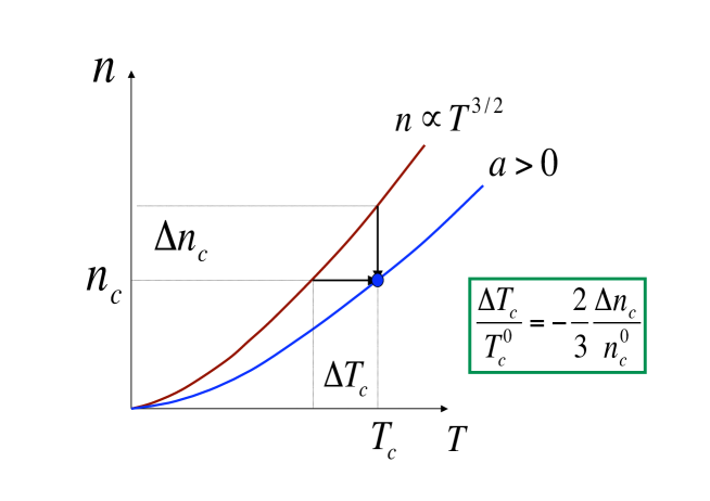
Figure 2: Expected change in the critical line caused by weak repulsive interactions characterized by a small scattering length $a$

In the previous lecture, we have seen that, under appropriate conditions, the effective hamiltonian is of the form

$$H=\int{d^{3}{\bf r}}\left\{\psi^{\dagger}({\bf r})\left(\-{\mbox{\boldmath$\nabla$}^{2}\over 2m}\,\!-\!\mu\right)\psi({\bf r})+{g_{0}\over 2}\psi^{\dagger}({\bf r})\psi^{\dagger}({\bf r})\psi({\bf r})\psi({\bf r})\right\},$$

where $g_{0}$ is related to the scattering length by (see eq. (46)):

$${1\over g_{R}}={1\over g_{0}}+{m\Lambda\over 2\pi^{2}},\qquad g_{R}={4\pi a\over m}.$$ (66)

This effective hamiltonian provides an accurate description of phenomena where the dominant degrees of freedom have long wavelength, $kr_{0}\ll 1$, and the system is dilute, $an^{1/3}\ll 1$. Recall also that we shall be working in the vicinity of the transition where $n^{1/3}\lambda\simeq 1$, with $\lambda$ the thermal wavelength.

3.1 Condensation condition and critical density

In order to exploit standard techniques of quantum field theory and many-body physics (see e.g.FW ; KB ; self-consistent ; BR ), we shall first relate the particle density to the single particle propagator. The particle density can be written as

$$n = \langle\psi^{\dagger}({\bf r})\psi({\bf r})\rangle,$$ (67)

$$= \lim_{\tau\to 0_{-}}\langle{\rm T}\psi(\tau,{\bf r})\psi^{\dagger}(0,{\bf r})\rangle=\lim_{\tau\to 0_{-}}G(\tau,0),$$

where

$$\psi^{\dagger}(\tau,{\bf r})={\rm e}^{\tau H}\psi^{\dagger}({\bf r}){\rm e}^{-\tau H},\qquad\qquad\psi(\tau,{\bf r})={\rm e}^{\tau H}\psi({\bf r})\,{\rm e}^{-\tau H},$$ (68)

are respectively the creation and annihilation operators in the Heisenberg representation and T denotes (imaginary) time ordering (see e.g. BR ). The single particle propagator is

$$G(\tau_{1}-\tau_{2},{\bf r_{1}-r_{2}}) = \langle{\rm T}\psi(\tau_{1},{\bf r_{1}})\psi^{\dagger}(\tau_{2},{\bf r_{2}})\rangle$$ (69)

$$= {\rm Tr}\left({{\rm e}^{-\beta H}\over Z}{\rm T}\psi(\tau_{1},{\bf r_{1}})\psi^{\dagger}(\tau_{2},{\bf r_{2}})\right).$$

It is a periodic function of $\tau=\tau_{1}-\tau_{2}$: for $0<\tau<\beta$, $G(\tau-\beta,{\bf r})=G(\tau,{\bf r})$, where $\beta=1/T$ is the inverse temperature. Because of its periodicity, it can be represented by a Fourier series

$$G(\tau,{\bf p})=T\sum_{n}e^{-i\omega_{n}\tau}G_{\alpha}(i\omega_{n},{\bf p}),$$ (70)

where the $\omega_{n}$’s are called the Matsubara frequencies:

$$\omega_{n}=2n\pi T,$$ (71)

and we have also taken a Fourier transform with respect to the spatial coordinates. We are making here an abuse of notation: we denote by the same symbol the function and its Fourier transform, with the implicit understanding that the arguments, whether space-time or energy-momentum variables, are enough to specify which function one is considering. The inverse transform is given by

$$G(i\omega_{n},{\bf p})=\int_{0}^{\beta}{\rm d}\tau\,e^{i\omega_{n}\tau}G(\tau,{\bf p}).$$ (72)

In the absence of interactions, the hamiltonian is of the form

$$H_{0}-\mu N = \int d^{3}{\bf r}\;\psi^{\dagger}({\bf r})\left(-{\hbar^{2}\mbox{\boldmath$\nabla$}^{2}\over 2m}-\mu\right)\psi({\bf r})$$ (73)

$$= \sum_{\bf p}\left(\varepsilon^{0}_{\bf p}-\mu\right)a^{\dagger}_{\bf p}a_{\bf p}=\sum_{p}\;\varepsilon_{\bf p}\,a^{\dagger}_{\bf p}a_{\bf p},$$

where

$$\psi({\bf r})=\sum_{\bf p}\,{{\rm e}^{i{\bf p\cdot\bf r}}\over\sqrt{\cal V}}\,a_{\bf p},\qquad\psi^{\dagger}({\bf r})=\sum_{\bf p}\,{{\rm e}^{-i{\bf p\cdot\bf r}}\over\sqrt{\cal V}}\,a^{\dagger}_{\bf p},\qquad\varepsilon^{0}_{\bf p}={{\bf p}^{2}\over 2m}.$$ (74)

In these formulae, ${\cal V}$ is the volume of the system, and the creation and annihilation operators satisfy $[a_{\bf p},a^{\dagger}_{\bf p^{\prime}}]=\delta_{\bf p,\bf p^{\prime}}$. The free single particle propagator can be obtained by a direct calculation. It reads

$$G^{-1}_{0}(i\omega_{n},{\bf p})=\varepsilon_{\bf p}-i\omega_{n},$$ (75)

or, in imaginary time,

$$G_{0}(\tau_{1}-\tau_{2},{\bf p}) = \langle{\rm T}a_{\bf p}(\tau_{1})a_{\bf p}^{\dagger}(\tau_{2})\rangle_{0}$$ (76)

$$= e^{-\varepsilon_{\bf p}(\tau_{1}-\tau_{2})}\left[(1+n_{\bf p})\theta(\tau_{1}-\tau_{2})+n_{\bf p}\theta(\tau_{2}-\tau_{1})\right],$$

where:

$$n_{\bf p}\equiv\langle a^{\dagger}_{\bf p}a_{\bf p}\rangle_{0}={{\rm Tr}{\rm e}^{-\beta(H_{0}-\mu N)}a^{\dagger}_{\bf p}a_{\bf p}\over{\rm Tr}{\rm e}^{-\beta(H_{0}-\mu N)}}={1\over e^{\beta\varepsilon_{\bf p}}-1},\qquad\varepsilon_{\bf p}=\varepsilon_{\bf p}^{0}-\mu.$$ (77)

Thus, for non interacting particles,

$$\lim_{\tau\to 0_{-}}G_{0}(\tau,{\bf p})=n_{\bf p},$$ (78)

so that the formula (67) yields the familiar formula (4) of the density.

The full propagator is related to the bare propagator by Dyson’s equation

$$G^{-1}(i\omega_{n},{\bf p})=G_{0}^{-1}(i\omega_{n},{\bf p})+\Sigma(i\omega_{n},{\bf p}),$$ (79)

where $\Sigma(i\omega,{\bf p})$ is the self-energy. In this case eq. (67) yields the following expression for the density

$$n=\lim_{\tau\to 0_{-}}T\sum_{n}\int{d^{3}{\bf p}\over(2\pi)^{3}}{e^{-i\omega_{n}\tau}\over\varepsilon_{\bf p}-i\omega_{n}+\Sigma(i\omega_{n},{\bf p})}.$$ (80)

or equivalently the occupation factor in the interacting system

$$n_{\bf p}=\lim_{\tau\to 0_{-}}T\sum_{n}e^{-i\omega_{n}\tau}G(i\omega_{n},{\bf p}).$$ (81)

We shall approach the condensation from the high temperature phase. Then the system remains in the normal state all the way down to $T_{c}$. The Bose-Einstein condensation occurs when the chemical potential reaches a value such that (see e.g. PPbook ):

$$G^{-1}(\omega=0,{\bf p}=0)=0\quad{\rm or}\quad\Sigma(\omega=0,{\bf p}=0)=\mu\,.$$ (82)

At that point,

$$G^{-1}(i\omega_{n},{\bf p})=i\omega_{n}-\varepsilon_{\bf p}^{0}-\left[\Sigma(i\omega_{n},{\bf p})-\Sigma(0,0)\right].$$ (83)

By using the general relation (80) between the Green function and the density, one can then write the following formula for the shift $\Delta n_{c}$ in the critical density caused by the interaction:

$$\Delta n_{c} = \lim_{\tau\to 0_{-}}T\sum_{n}e^{-i\omega_{n}\tau}\!\int{d^{3}{\bf p}\over(2\pi)^{3}}$$ (84)

$$\times\left\{{1\over\varepsilon_{\bf p}^{0}+\Sigma(i\omega_{n},{\bf p})-\Sigma(0,0)-i\omega_{n}}-{1\over\varepsilon_{\bf p}^{0}-i\omega_{n}}\right\}.$$

The first term in this expression is the critical density of the interacting system at temperature $T$, the second term is the critical density of the non interacting system at the same temperature. This formula makes it obvious that $\Delta n_{c}$ vanishes if the self-energy is independent of energy and momentum. This is the case in particular when the interactions are treated at the mean field level, as we already observed. In this case, $\Sigma=2gn$, and the formula above yields

$$\Delta n_{c}=\int{d^{3}{\bf p}\over(2\pi)^{3}}\left\{{1\over{\rm e}^{\beta(\varepsilon_{\bf p}^{0}+2gn-\mu_{c})}-1}-{1\over{\rm e}^{\beta\varepsilon_{\bf p}^{0}}-1}\right\}=0,$$ (85)

which vanishes since $\mu_{c}=2gn$.

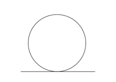
Figure 3: The contribution to the self-energy $\Sigma$ that is of leading order in $a$

3.2 Breakdown of perturbation theory

Because the interactions are weak, one may imagine calculating $\Delta n_{c}$ by perturbation theory. However the perturbative expansion for a critical theory does not exist for any fixed dimension $d<4$; infrared divergences prevent a complete calculation, as we shall recall. If one introduces an infrared cutoff $k_{c}$ to regulate the momentum integrals, one finds that perturbation theory breaks down when $k_{c}\sim a/\lambda^{2}$, all terms being then of the same order of magnitude.

The leading order on $a$ is given by the diagram in Fig. 3. As we just saw, the contribution of this diagram to $\Sigma$ is just the mean field value $2gn$, and the net effect on $\Delta n_{c}$ is zero. We shall then examine the second order contribution, given by the diagram displayed in Fig. 4. We shall see that this diagram is infrared divergent. Next, we shall show, using simple power counting, that such infrared divergences occur in higher orders and signal a breakdown of perturbation theory as one approaches the critical point.

Second order perturbation theory

The second order self-energy diagram is the lowest order diagram that is momentum dependent and can therefore yield corrections to the critical density. It is displayed in Fig. 4.

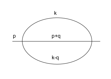
Figure 4: The contribution to the self-energy $\Sigma$ that is, a priori, of second order in $a$

Its contribution is given by

$$\Sigma(i\omega_{n},{\bf p}) = -2g^{2}T^{2}\sum_{n^{\prime}n^{\prime\prime}}\int{d^{3}{\bf k}\over(2\pi)^{3}}{d^{3}{\bf q}\over(2\pi)^{3}}$$

$$\times {1\over\varepsilon_{\bf k-q}-i(\omega_{n^{\prime}}-\omega_{n^{\prime\prime}})}\,{1\over\varepsilon_{\bf k}-i\omega_{n^{\prime}}}\,{1\over\varepsilon_{\bf p+q}-i(\omega_{n}+\omega_{n^{\prime\prime}})}.$$

Anticipating that infrared divergence can occur, we focus on the contribution where $\omega_{n^{\prime}}=\omega_{n^{\prime\prime}}=0$, and calculate the difference $\Sigma(i\omega_{n}=0,{\bf p})-\Sigma(i\omega_{n}=0,{\bf p}=0)$, which we write from now on simply as $\Sigma_{cl}({\bf p})-\Sigma_{cl}(0)$:

$$\Sigma_{cl}({\bf p})-\Sigma_{cl}(0) = -2g^{2}T^{2}\int{d^{3}{\bf k}\over(2\pi)^{3}}{d^{3}{\bf q}\over(2\pi)^{3}}$$

$$\times {1\over(\varepsilon^{0}_{\bf k-q}-\mu^{\prime})(\varepsilon^{0}_{\bf k}-\mu^{\prime})}\left[{1\over\varepsilon^{0}_{\bf p+q}-\mu^{\prime})}-{1\over\varepsilon^{0}_{\bf q}-\mu^{\prime}}\right].$$

In this calculation we have used Hartree-Fock propagators, and set

$$\mu^{\prime}=\mu-\Sigma_{HF}\equiv-{k_{c}^{2}\over 2m},$$ (88)

where $\Sigma_{HF}=2gn$. The quantity $k_{c}$, whose significance will appear more clearly as we progress in the discussion, plays the role of an infrared cutoff in the integrals. Note that $k_{c}\rightarrow 0$ ($\mu^{\prime}\rightarrow 0$) when $T\rightarrow T_{c}^{0}$. With this new notation

$$\varepsilon^{0}_{k}-\mu^{\prime}=(k^{2}+k_{c}^{2})/2m.$$ (89)

We shall also set

$$U(p)\equiv 2m(\Sigma_{cl}(p)-\Sigma_{cl}(0)).$$ (90)

The integral in eq. (LABEL:sigsumnew) can be calculated analytically (see bigbec ) and yields

$$U(p)=128\pi^{2}\left({a\over\lambda^{2}}\right)^{2}\left\{{3k_{c}\over p}{\arctan}{p\over 3k_{c}}+{1\over 2}\ln\left[1+\left({p\over 3k_{c}}\right)^{2}\right]-1\right\}.$$ (91)

This equation shows that $U(p)$ is a monotonically increasing function of $p$, $\sim p^{2}$ at small $p$, and growing logarithmically at large $p$. This logarithmic behavior, obtained in perturbation theory, remains in general the dominant behavior of $U(p)$ at large $p$, i.e., for $k_{c}\ll p\,\raisebox{-2.15277pt}{$\stackrel{{\scriptstyle<}}{{\sim}}$}\,1/\lambda$. This equation (91) also reveals the anticipated infrared divergence: $U(p)$ diverges logarithmically as $k_{c}\to 0$.

The condensation condition (82), $\mu^{\prime}=\Sigma_{cl}(0)$, reads

$$k_{c}^{2}\approx 128\pi^{2}\left({a\over\lambda^{2}}\right)^{2}\left[\ln\left({\Lambda\over 3k_{c}}\right)-\gamma\right],$$ (92)

where the right hand side is $-2m\Sigma_{cl}(0)$, $\gamma=0.577\ldots$ is Euler’s constant, and the approximate equality is valid when $\Lambda\gg k_{c}$, which we assume to be the case. Here $\Lambda$ is an ultraviolet cut-off that we have introduced to handle the divergence of $\Sigma_{cl}(0)$, and whose origin is the neglect of the non vanishing Matsubara frequencies. Typically, $\Lambda\sim 1/\lambda$. Eq. (92) shows that $k_{c}\sim a/\lambda^{2}$ when $a$ is small bigbec .

This simple calculation illustrates the limits of a pertubative approach. The infrared cutoff $k_{c}\sim a/\lambda^{2}$ introduces spurious $a$ dependence. The condensation condition which relates the infrared cutoff to the microscopic length $\lambda$, induces a spurious logarithmic correction which does not vanish as $a\to 0$. In fact such logarithms do appear as higher order corrections, as we shall see later, but are absent in the leading order result.

Higher orders

The infrared divergences that we have identified in the second order calculation persist, and worsen, in higher order contributions. This may be seen by using a simple power counting argument. Let us first consider diagrams in which all the internal lines carry vanishing Matsubara frequencies. We use again HF propagators so that all the functions that are integrated in the diagrams are products of fractions of the form

$$\left[K^{2}+k_{c}^{2}\right]^{-1},$$ (93)

where $K$ denotes a generic combination of momenta; it is then natural to use the dimensionless products $K/k_{c}$ as new integration variables. Consider then a diagram of order $a^{n}$. The lowest order $n=2$ has just been calculated, and, for large $p/k_{c}$, it is proportional to $(a/\lambda)^{2}\ln(p/k_{c})$, where $p$ is the external momentum. For $n>2$, every additional order brings in one factor $a$ from the vertex, one integration over three-momenta, a factor $T$, and two internal propagators. The contribution of the diagram can thus be written as:

$$T\,\left({a\over\lambda}\right)^{2}\left({a\over k_{c}\lambda^{2}}\right)^{n-2}F(p/k_{c}),$$ (94)

where $F$ is a dimensionless function, which we do not explicitly need here. The main point is that when one approaches the critical temperature, the coherence length becomes large so that the summation of terms (94) diverges. In the critical region, $k_{c}\sim a/\lambda^{2}$, so that all the terms in the perturbative expansion are of the same order of magnitude. Therefore, at the critical point, perturbation theory is not valid.

Let us now assume that in a given diagram some propagators carry non-zero Matsubara frequencies so that one momentum integration ($k$) will be altered. For that integration, the presence of a non vanishing Matsubara frequency in the denominators of the propagators ensures that no singularity at $k=0$ can take place. Essentially, in the corresponding propagators, $k_{c}$ is replaced by a term proportional to $1/\lambda$, so that one factor $a/\lambda^{2}k_{c}$ in (94) is now replaced by $a/\lambda$. Compared to the diagram with only vanishing Matsubara frequencies, this diagram is down by a factor $a/\lambda$, and thus negligible in a leading order calculation of $\Sigma$. This reasoning generalizes trivially to diagrams containing more non vanishing Matsubara frequencies.

Formula for $\Delta n_{c}$

It follows from the previous discussion that in order to obtain the leading order shift in the critical density, one may retain in eq. (80) the contribution of the zero Matsubara frequency only. That is,

$$\Delta n_{c} \simeq T\int{d^{3}p\over(2\pi)^{3}}\left\{{1\over\varepsilon_{p}+\Sigma_{cl}(p)-\Sigma_{cl}(0)}-{1\over\varepsilon_{p}}\right\}$$ (95)

$$\simeq -{2\over\pi\lambda^{2}}\int_{0}^{\infty}dp{U(p)\over p^{2}+U(p)},$$

with $U(p)$ given by eq. (90). Note that this integral is finite: $U(p)\sim\ln p$ at large $p$, and $p^{2}+U(p)\sim p^{2-\eta}$ at small $p$. Note also that since $U(p)>0$ (in fact the general qualitative behavior of $U(p)$ is correctly given by eq. (91)), the correction $\Delta n_{c}$ is negative, implying a positive shift of $T_{c}$.

3.3 Classical field approximation

Once restricted to their zero Matsubara frequency components, the fields $\psi$ and $\psi^{\dagger}$ can be considered as classical fields, and the entire calculation can be cast in terms of a classical field theory. To see that, let us expand the field variables in the path integral (52) in terms of their Fourier components:

$$\psi(\tau,{\bf r})=\psi_{0}({\bf r})+T\sum_{n\neq 0}{\rm e}^{-i\omega_{n}\tau}\psi_{n}({\bf r}),$$ (96)

where the $\omega_{n}$’s are the Matsubara frequencies, and we have called $\psi_{0}({\bf r})$ the $\tau$-independent part of the field.

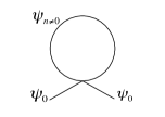
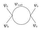
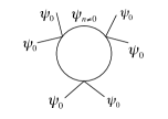
Figure 5: Some diagrams contributing to the parameters of the effective theory. The external legs represent the field $\psi_{0}$ carrying vanishing Matsubara frenqency. The internal lines carry non vanishing Matsubara frequencies $\omega_{n}$. The first diagram from the left is a correction to the chemical potential; it is of order $a$, but does not contribute to the shift in $T_{c}$. The second diagram is a correction to the $\psi_{0}^{4}$ coupling constant. The last diagram is the contribution to the $\psi^{6}$ vertex. The last two contributions are of order $a^{2}$ and $a^{3}$ respectively, and can be ignored in a leading order analysis.

The partition function (52) can then be written as:

$$Z\,=\,{\cal N}_{1}\int{\cal D}\psi_{0}\exp\left\{-S_{\rm eff}[\psi_{0}]\right\}\,,$$ (97)

where $\psi_{0}$ depends only on spatial coordinates, and

$$\exp\left\{-S_{\rm eff}[\psi_{0}]\right\}=\,{\cal N}_{2}\int{\cal D}\psi_{n\neq 0}\,{\rm e}^{-{\cal S}}\,$$ (98)

where ${\cal S}$ is the action (2.5). ${\cal N}_{1}$ and ${\cal N}_{2}$ are (infinite) normalization constants. The quantity $S_{\rm eff}[\psi_{0}]$ is the effective action for $\psi_{0}$. Aside from the direct classical field contribution to which we shall return shortly, this effective action receives also contributions which, diagrammatically, correspond to connected diagrams whose external lines are associated to $\psi_{0}$, and the internal lines are the propagators of the non-static modes $\psi_{n}$. A few examples are displayed in Fig. 5. Thus, a priori, $S_{\rm eff}[\psi_{0}]$ contains operators of arbitrarily high order in $\psi_{0}$. In the present case, however, it is easy to verify that the contributions beyond those kept in the classical action, are of higher order in $a$, and can therefore be ignored in a leading order calculation.

The strategy which consists of integrating out the non-static modes in perturbation theory in order to obtain an effective three-dimensional theory for the soft static modes, is referred to, in another context, as “dimensional reduction” (see e.g. Gins80 ; Appel81 ; Nadkarni83 ).

In leading order, the effective action is the restriction of eq. (2.5) to the static mode $\psi_{0}$ and the partition function (97) can be written as:

$$Z\,\approx\,{\cal N}\int{\cal D}\psi_{0}\,\exp\left\{-\beta\int{\rm d}^{3}r\,({\cal H}({\bf r})-\mu{\cal N}({\bf r}))\right\}\,,$$ (99)

where $\psi_{0}({\bf r})$ is a three-dimensional field, and

$${\cal H-\mu N}\,=\,{|\mbox{\boldmath$\nabla$}\psi_{0}|^{2}\over 2m}-\mu^{\prime}\,|\psi_{0}|^{2}+{g_{0}\over 2}(|\psi_{0}|^{2})^{2}\,.$$ (100)

We shall refer to this limit as the classical field approximation. The zero Matsubara component of the density is given by $\langle|\psi_{0}(r)|^{2}\rangle$, which diverges in the effective theory. However, recall that by assumption, the wavenumbers of the classical field are limited to $k$ less than an ultraviolet cutoff $\Lambda\sim\lambda^{-1}$. In fact we shall not need to use a cut-off since the variation of the critical density is a finite quantity (see eq. (110) below).

• Remark.

  Ignoring the time dependence of the fields is equivalent to retaining only the zero Matsubara frequency in their Fourier decomposition. Then the Fourier transform of the free propagator is simply:

  $$G_{0}({\bf p})\,=\,{T\over\varepsilon_{\bf p}}\,.$$ (101)

  This may be obtained directly from (70) and (75) keeping only the term with $\omega_{n}=0$, or from eq. (99). The classical field approximation corresponds also to the following approximation of the statistical factor (see eq. (81))

  $$n_{\bf p}={1\over{\rm e}^{\beta\varepsilon_{\bf p}}-1}\approx{T\over\varepsilon_{\bf p}}\,.$$ (102)

  Both approximations make sense only for $\varepsilon_{\bf p}\ll T$, implying $n_{\bf p}\gg 1$. In this limit, the energy per mode is $\propto\varepsilon_{\bf p}n_{\bf p}\approx T$, as expected from the classical equipartition theorem. This long wavelength limit can also be viewed as a high temperature limit (the time dependence of the field becomes indeed unimportant as $\beta\to 0$).

  One should not confuse this classical field approximation with the classical limit reached when the thermal wavelength of the particles becomes small compared to their average separation distances. In this limit, the occupation of the single particle states becomes small, and the statistical factors can be approximated by their Boltzmann form:

  $${1\over{\rm e}^{\beta(\varepsilon_{p}-\mu)}\pm 1}\approx{\rm e}^{\beta(\varepsilon_{p}-\mu)}\ll 1,$$ (103)

  where we have used the fact that ${\rm e}^{-\beta\mu}$ is large in the classical limit.

At this point it is easy to understand the origin of the breakdown of perturbations theory. The critical region is characterized by the fact that all the terms in the integrand of (100) become of the same order of magnitude. This occurs for $k\mathrel{\hbox to0.0pt{\raise 2.20013pt\hbox{$<$}\hss}{\lower 2.20013pt\hbox{$\sim$}}}k_{c}$, with $k_{c}$ such that:

$${k_{c}^{2}\over 2m}\sim\mu^{\prime}\sim{a\over m}{T\over\mu^{\prime}}k_{c}^{3},$$ (104)

where $(T/\mu^{\prime})k_{c}^{3}$ is the contribution to the density of the modes with $k\sim k_{c}$. From eq. (104) we see that $k_{c}\sim a/\lambda^{2}$. For $k\simeq k_{c}$ perturbation theory in $a$ makes no sense, and in fact all terms in the perturbative expansion are infrared divergent. For $k_{c}\ll k\ll\lambda^{-1}$, perturbation theory is applicable.

• Remark. In a trap the effect of critical fluctuations is subleading. To see that let us estimate the size of the critical region in a trap arnold01 . Recall that at the transition the thermal wavelength is $\lambda\sim a_{ho}N^{-1/6}$, where $a_{ho}=1/\sqrt{m\omega_{0}}$ is the characteristic size of the harmonic oscillator trap (see the discussion after eq. (30)), and the size $R_{cl}$ of the thermal cloud where most of the particles sit is $R_{cl}\sim a_{ho}N^{1/6}\sim\lambda N^{1/3}$. According to eq. (104), the critical region is reached when the chemical potential deviates from its critical value by an amount $\mathrel{\hbox to0.0pt{\raise 1.98012pt\hbox{$<$}\hss}{\lower 1.98012pt\hbox{$\sim$}}}k_{c}^{2}/{2m}\sim a^{2}/(m\lambda^{4})$. In a trap the effective local potential is of the form $\mu-{1\over 2}m\omega_{0}^{2}r^{2}$. Taking $\mu$ at its critical value, one finds that the particles will be in the critical region as long as $r\mathrel{\hbox to0.0pt{\raise 1.98012pt\hbox{$<$}\hss}{\lower 1.98012pt\hbox{$\sim$}}}R_{cr}$ with $m\omega_{0}^{2}R_{cr}^{2}\sim a^{2}/(m\lambda^{4})$, or $R_{cr}\sim a(a_{ho}/\lambda)^{2}\sim aN^{1/3}$. Thus the relative size of the critical region is $R_{cr}/R_{cl}\sim a/\lambda$, and the ratio of the particles in the critical region to the total number of particles is $\sim(a/\lambda)^{3}$. Under such conditions, it can be shown that one can use perturbation theory to estimate the corrections due to the interactions to the relation (4) in a trap; the resulting contributions to the shift of $T_{c}$ are then subleading in $a$, as compared to the mean field effect discussed in the first lecture arnold01 .

In view of the forthcoming discussions, it is convenient to rescale the field $\psi_{0}$ and to parametrize it in terms of two real fields $\varphi_{1},\varphi_{2}$: $\psi_{0}=\sqrt{mT}(\varphi_{1}+i\varphi_{2})$. The partition function then reads

$${\cal Z}=\int{\cal D}\varphi\,{\rm e}^{-{\cal S}},$$ (105)

where ${\cal S}(\varphi)=(H-\mu N)/T$ is given by: :

$${\cal S}\left(\varphi\right)=\int\left\{{1\over 2}\left[\partial_{\mu}\varphi(x)\right]^{2}+{1\over 2}r\phi^{2}(x)+{u\over 4!}\left[\varphi^{2}(x)\right]^{2}\right\}{\rm d}^{d}x\,,$$ (106)

where $\varphi^{2}=\varphi_{1}^{2}+\varphi_{2}^{2}$ and:

$$r=-2mT\mu,\qquad u=96\pi^{2}{a\over\lambda^{2}}.$$ (107)

In eq. (106) we have kept the dimension $d$ of the spatial integration arbitrary for the convenience of forthcoming discussions. The single particle Green’s function $G(p)$ is related to the inverse two-point function $\Gamma^{(2)}(p)$ of the classical field theory by

$$2mTG^{-1}(p)=\Gamma^{(2)}(p),\qquad p^{2}+U(p)=\Gamma^{(2)}(p)-\Gamma^{(2)}(0).$$ (108)

As it stands this field theory suffers from UV divergences. These are absent in the original theory, the higher frequency modes providing a large momentum cutoff $\sim 1/\lambda$. This cutoff may be restored when needed, but, as we show later, since the shift of the critical temperature is dominated by long distance properties it is independent of the precise cutoff procedure.

We shall also find useful to consider the $O(N)$ symmetric generalization of the Euclidean action (106). The field $\varphi(x)$ then has $N$ real components, and, e.g.,

$$\varphi^{2}=\sum_{i=1}^{N}\varphi_{i}^{2}\,,$$ (109)

and the shift in the critical density is given by

$$\Delta n_{c} = 2mT\sum_{i=1}^{N}\left[\left<\phi_{i}^{2}\right>_{a\neq 0}-\left<\phi_{i}^{2}\right>_{a=0}\right]$$ (110)

$$= {2mT\,N\,}\int{{\rm d}^{d}p\over(2\pi)^{d}}\,\left({1\over\Gamma^{(2)}(p)}-{1\over p^{2}}\right),$$

with $\delta_{ij}/{\Gamma^{(2)}(k)}$ the connected two-point correlation function.

The advantage of this generalization is that it provides us with a tool, the large $N$ expansion, which allows us to calculate at the critical point (for a recent review see e.g. Moshe:2003xn ).

Linear dependence of the density correction

It is now easy to see the origin of the linear relation between $\Delta n_{c}$ and $a$. Note first that the action (106) contains a single dimensionfull parameter, $u$, $r$ being adjusted for any given $u$ to be at criticality. In fact the effective three dimensional theory is ultraviolet divergent, so there is a priori another parameter, the ultraviolet cut-off $\Lambda\sim 1/\lambda$. It follows then from dimensional analysis that $U(p)$ defined in eq. (90) can be written as

$$U(p=xu)=u^{2}\sigma(x,u/\Lambda).$$ (111)

Now, the diagrams involved in the calculation of $U$ are ultraviolet convergent, so that $U$ is in fact independent of the cut-off $\Lambda$, and the infinite cut-off limit can be taken. Note however that the validity of the classical field approximation requires that all momenta involved in the various integrations are small in comparison with $\Lambda\sim\lambda^{-1}$ or, in other words, that the integrands are negligibly small for momenta $k\sim\lambda^{-1}$. Only then can we ignore the effects of non vanishing Matsubara frequencies and use for instance the approximate form of the statistical factors (102). In other words, the infinite cut-off limit is meaningful only if letting the cut-off becoming bigger than $\lambda^{-1}$ does not affect the results. This implies that $u\lambda\sim a/\lambda$ is sufficiently small.

In the region of validity of the classical field approximation, that is, for small enough $u$, $\sigma(x,u/\Lambda)$ becomes a universal function $\sigma(x)$, independent of $u$, and $\Delta n_{c}$ in eq. (95) takes the form

$$\Delta n_{c}=-{2u\over\pi\lambda^{2}}\int dx{\sigma(x)\over x^{2}+\sigma(x)},$$ (112)

showing that the change in the critical density is indeed linear in $a$.

Renormalization group argument

The linearity of the relation between the shift in $T_{c}$ and the scattering length can also be understood from a simple renormalization group analysis. Let us introduce a large momentum cutoff $\Lambda\sim 1/\lambda$, and a dimensionless coupling constant $g$

$$g=\Lambda^{d-4}u\propto\left(a\over\lambda\right)^{d-2}\,.$$ (113)

At $T_{c}$ the two-point function in momentum space satisfies the renormalization group equation Zinn-Justin:2002ru

$$\left(\Lambda{\partial\over\partial\Lambda}+\beta(g){\partial\over\partial g}-\eta(g)\right)\Gamma^{(2)}(p,\Lambda,g)=0\,.$$ (114)

This equation, together with dimensional analysis, implies that the two-point function has the general form

$$\Gamma^{(2)}(p,\Lambda,g)=p^{2}Z(g)F\bigl{(}p/k_{c}\bigr{)},$$ (115)

where $k_{c}=k_{c}(g)$ is a function of $g$ which, on dimensional grounds, is proportional to $\Lambda$, so that $\Lambda\partial_{\Lambda}k_{c}=k_{c}$. The ansatz (115) for $\Gamma^{(2)}(p,\Lambda,g)$ provides then a solution of eq. (114) if $Z(g)$) and $k_{c}(g)$ obey the equations

$${\partial\ln Z(g)\over\partial g} = {\eta(g)\over\beta(g)},$$ (116)

$${\partial\ln k_{c}(g)\over\partial g} = -{1\over\beta(g)}\,.$$ (117)

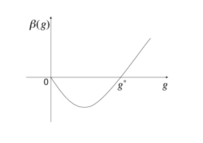
Figure 6: The $\beta$-function with the two fixed points at $g=0$ and $g=g^{*}$.

Since $\beta(g)=-(4-d)g+(N+8)g^{2}/48\pi^{2}+{\cal O}(g^{3})$, $\beta(g)$ is of order $g$ for small $g$ in $d<4$; similarly $\eta(g)=(N+2)g^{2}/(72(8\pi^{2})^{2})+{\cal O}(g^{3})$. Therefore

$$Z(g)=\exp\int_{0}^{g}{\eta(g^{\prime})\over\beta(g^{\prime})}{\rm d}g^{\prime}=1+{\cal O}(g^{2});$$ (118)

to leading order $Z(g)$ =1. The function $k_{c}(g)$ is then obtained by integrating eq. (117),

$$k_{c}(g)=g^{1/(4-d)}\Lambda\exp\left[-\int_{0}^{g}{\rm d}g^{\prime}\left({1\over\beta(g^{\prime})}+{1\over(4-d)g^{\prime}}\right)\right].$$ (119)

In $d=3$,

$$k_{c}(g)=\Lambda{gg^{*}\over g^{*}-g},$$ (120)

where $g^{*}$ is the infrared fixed point (see Fig. 6). The scale $k_{c}(g)$ plays a specific role in the analysis as the crossover separating a universal long-distance regime, where

$$\Gamma^{(2)}(p)\propto p^{2-\eta}\qquad p\ll k_{c}(g),$$ (121)

governed by the non-trivial zero, $g^{*}$, of the $\beta$-function, from a universal short distance regime governed by the Gaussian fixed point, $g=0$, where

$$\Gamma^{(2)}(p)\propto p^{2}\qquad k_{c}(g)\ll p\ll\Lambda\,.$$ (122)

However such a regime exists only if $k_{c}(g)\ll\Lambda$, i.e., if there is an intermediate scale between the infrared and the microscopic scales; otherwise only the infrared behavior can be observed. In a generic situation $g$ is of order unity, and thus $k_{c}(g)$ is of order $\Lambda$, and the universal large momentum region is absent. Instead $k_{c}(g)\ll\Lambda$ implies that $g$ be small. Since $g\sim a/\lambda\ll 1$, see eq. (113), this condition is satisfied in the present situation.

It is then easy to show, repeating essentially the same analysis as before, that with this condition, $\Delta T_{c}\propto k_{c}(g)$. We set $p=xk_{c}(g)$, and find for the integral in eq. (110) the general form

$$\int{{\rm d}^{d}p\over(2\pi)^{d}}\,\left({1\over\Gamma^{(2)}(k)}-{1\over p^{2}}\right)=k_{c}(g)\int{{\rm d}^{3}x\over(2\pi)^{3}}{1\over x^{2}}\left({1\over F(x)}-{1}\right);$$ (123)

the $g$ dependence is entirely contained in $k_{c}(g)$, and for small $g$, $k_{c}(g)\simeq u$.

Recall that both the perturbative large momentum region and the non-perturbative infrared region contribute to the integrand in eq. (123), or equivalently in eq. (112), and that the functions $F(x)$ or $\sigma(x)$ cannot be calculated using perturbation theory.

The $1/N$ expansion allows an explicit calculation, and yields, in leading order for the coefficient $c$ in eq. (1) the value $c=2.3$ BigN . However, the best numerical estimates for $c$ are those which have been obtained using the lattice technique by two groups, with the results: $c=1.32\pm 0.02$ latt2 and $c=1.29\pm 0.05$ latt1 . The availabilty of these results has turned the calculation of $c$ into a testing ground for other non perturbative methods: expansion in $1/N$ BigN ; Arnold:2000ef , optimized perturbation theory Kneur04 ; souza , resummed perturbative calculations to high loop orders Kastening:2003iu . Note that while the latter methods yield critical exponents with several significant digits, they predict $c$ with only a 10% accuracy. This illustrates the difficulty of getting an accurate determination of $c$ using (semi) analytical techniques.

• Remark. The linear dependence in $a$ of the shift of $T_{c}$ holds only if $a$ is small enough, as we have already indicated. When $a$ is not small enough various corrections need to be taken into account that alter the simple linear law. In particular, corrections come from the non vanishing Matsubara frequencies, and their impact on the effective theory for $\psi_{0}$. Such corrections have been analyzed in detail in Arnold:2001nn (see also NEW ). The net result is the following expression for $\Delta T_{c}$:

  $${\Delta T_{c}\over T_{c}^{0}}=c(an^{1/3})+\left[c_{2}^{\prime}\ln(an^{1/3})+c_{2}^{\prime\prime}\right](an^{1/3})^{2}+{\cal O}(a^{3}n).$$ (124)

  Aside from such corrections, the evaluation of $\Delta T_{c}$ in higher order requires that one improves the accuracy of the effective hamiltonian and include for instance effective range corrections.

4 LECTURE 3 : The Non Perturbative Renormalization Group and the calculation of $c$

The analysis of the previous lectures has shown that the coefficient $c$ in the formula (1) can be written as:

$$c\,\equiv-{256\pi^{3}\over\left(\zeta(3/2)\right)^{4/3}}\,{\Delta\langle\varphi_{i}^{2}\rangle\over Nu},$$ (125)

where $\Delta\langle\varphi_{i}^{2}\rangle$ represents the change, due to interactions, of the fluctuations of the scalar field of the $O(N)$ symmetric model, and is given by:

$${\Delta\langle\varphi_{i}^{2}\rangle\over Nu}=-\int{{\rm}dx\over 2\pi^{2}}\,{\sigma(x)\over x^{2}+\sigma(x)},$$ (126)

where $\sigma(x)=u^{-2}U(p=xu)$ and $U(p)$ is essentially the self-energy of the field at criticality (see eqs. (110) and (108)). In order to get the numerical factor in eq. (125), we have combined eqs. (1), (64), (8) and (107). Eq. (125) has been written for arbitray $N$ in order to be able to compare with all available results. Bose-Einstein condensation corresponds to $N=2$.

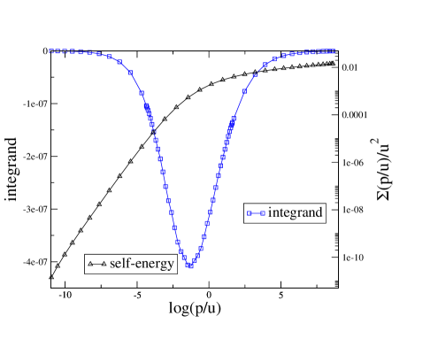
Figure 7: The function $\sigma(x=p/u)$ at criticality, and the integrand of eq. ( 126) as a function of $\ln(p/u)$, for $u\mathrel{\hbox to0.0pt{\raise 2.20013pt\hbox{$<$}\hss}{\lower 2.20013pt\hbox{$\sim$}}}10^{-4}$ for which $\sigma(x)$ is independent of $u$. From Ref. Blaizot:2004qa .

The integrand of eq. (126), calculated in the approximate scheme described in Blaizot:2004qa , is shown in Fig. 7. The minimum occurs at the typical scale $k_{c}$ which separates the scaling region from the high momentum region where perturbation theory applies. As we have already emphasized, the difficulty in getting a precise evaluation of the integral (126) is that it requires an accurate determination of $\sigma(x)$ in a large region of momenta including in particular the crossover region between two different physical regimes; as we have seen in the previous lecture, this cannot be done using perturbation theory, eventhough the coupling constant, $\sim a$, is small.

In this last lecture, I shall show how the non perturbative renormalization group (NPRG) can be used to calclate $\sigma(x)$. The NPRG Wetterich93 ; Ellwanger93 ; Tetradis94 ; Morris94 ; Morris94c (sometimes called “exact” or “functional”, depending on which aspect of the formalism one wishes to emphasize) stands out as a promising tool, suggesting new approximation schemes which are not easily formulated in other, more conventional, approaches in field theory or many body physics. It has been applied successfully to a variety of problems, in condensed matter, particle or nuclear physics (for reviews, see e.g. Bagnuls:2000ae ; Berges02 ; Canet04 ). In most of these problems however, the focus is on long wavelength modes and the solution of the NPRG equations involves generally a derivative expansion which only allows for the determination of the $n$-point functions and their derivatives essentially only at vanishing external momenta. This is not enough in the present situation where, as we have seen, a full knowledge of the momentum dependence of the 2-point function is required. We have therefore developed new methods to solve the NPRG equations. The following sections will briefly present some of the ingredients involved, without going into the technical details of their implementation. These can be found in Refs. Blaizot:2004qa ; Blaizot:2005wd ; Blaizot:2006vr ; Blaizot:2005xy ; Blaizot:2006ak , from which much of the material presented here is borrowed. For definiteness, we focus on the $O(N)$ symmetric scalar field theory with action (106). See also the lecture by H. Gies in this volume Gies:2006wv for further introduction to these techniques, and their application to other theories, in particular non-abelian gauge theories. Other applications of the renormalization group to Bose-Einstein condensation can be found in Stoof2 ; Andersen:1998bc ; Andersen:1999dy .

4.1 The NPRG equations

The NPRG allows the construction of a set of effective actions $\Gamma_{\kappa}[\phi]$ which interpolate between the classical action $S$ and the full effective action $\Gamma[\phi]$: In $\Gamma_{\kappa}[\phi]$ the magnitude of long wavelength fluctuations of the field is controlled by an infrared regulator depending on a continuous parameter $\kappa$ which has the dimension of a momentum. The full effective action is obtained for the value $\kappa=0$, the situation with no infrared cut-off. In the other limit, corresponding to a value of $\kappa$ of the order of the microscopic scale $\Lambda$ at which fluctuations are suppressed, $\Gamma_{\kappa=\Lambda}[\phi]$ reduces to the classical action .

In practice the fluctuations are controlled by adding to the classical action (106) the $O(N)$ symmetric regulator

$$\Delta S_{\kappa}[\varphi]={1\over 2}\int{{\rm d}^{d}q\over(2\pi)^{d}}\,\varphi_{i}(q)\,R_{\kappa}(q)\,\varphi_{i}(-q),$$ (127)

where $R_{\kappa}$ denotes a family of “cut-off functions” depending on $\kappa$. As we just said, the role of $\Delta S_{\kappa}$ is to suppress the fluctuations with momenta $q\mathrel{\hbox to0.0pt{\raise 2.20013pt\hbox{$<$}\hss}{\lower 2.20013pt\hbox{$\sim$}}}\kappa$, while leaving unaffected those with $q\mathrel{\hbox to0.0pt{\raise 2.20013pt\hbox{$>$}\hss}{\lower 2.20013pt\hbox{$\sim$}}}\kappa$. Thus, typically, $R_{\kappa}(q)\to\kappa^{2}$ when $q\ll\kappa$, and $R_{\kappa}(q)\to 0$ when $q\mathrel{\hbox to0.0pt{\raise 2.20013pt\hbox{$>$}\hss}{\lower 2.20013pt\hbox{$\sim$}}}\kappa$. There is a large freedom in the choice of $R_{\kappa}(q)$, abundantly discussed in the literature Ball95 ; Comellas98 ; Litim ; Canet02 . The choice of the cut-off function matters when approximations are done, as is the case in all situations of practical interest. Most of the results that will be presented here have been obtained with the cut-off function proposed in Litim :

$$R_{\kappa}(q)\propto(\kappa^{2}-q^{2})\theta(\kappa^{2}-q^{2}).$$ (128)

This regulator has the advantage of allowing some calculations to be done analytically.

For each value of $\kappa$, one defines the generating functional of connected Green’s functions

$$W_{\kappa}[J]=\ln\int D\varphi\hskip 2.84544pt\exp\left\{{-S[\varphi]-\Delta S_{\kappa}[\varphi]+\int d^{d}x\varphi(x)J(x)}\right\}.$$ (129)

The Feynman diagrams contributing to $W_{\kappa}$ are those of ordinary perturbation theory, except that the propagators contain the infrared regulator. We also define the effective action, through a modified Legendre transform that includes the explicit subtraction of $\Delta S_{\kappa}$:

$$\Gamma_{\kappa}[\phi]=-W_{\kappa}[J_{\phi}]+\int d^{d}x\hskip 2.84544pt\phi(x)J_{\phi}(x)-\Delta S_{\kappa}[\phi],$$ (130)

where $J_{\phi}$ is obtained by inverting the relation

$$\phi_{\kappa,J}(x)\equiv\left\langle\varphi(x)\right\rangle_{\kappa,J}={\delta W_{\kappa}\over\delta J(x)}.$$ (131)

for $\phi_{\kappa,J}(x)=\phi$. Note that, in this inversion, $\phi$ is considered as a given variable, so that $J_{\phi}$ becomes implicitly dependent on $\kappa$. Taking this in to account, it is easy to derive the following exact flow equation for $\Gamma_{\kappa}[\phi]$:

$$\partial_{\kappa}\Gamma_{\kappa}[\phi]={1\over 2}{\rm tr}\int{d^{d}q\over(2\pi)^{d}}\,\partial_{\kappa}R_{\kappa}(q)\,G(\kappa,q),$$ (132)

where the trace ${\rm tr}$ runs over the O($N$) indices, and

$$G^{-1}_{ij}(q;\kappa;\phi)=\Gamma^{(2)}_{ij}(\kappa;q;\phi)+\delta_{ij}R_{\kappa}(q).$$ (133)

with $\Gamma^{(2)}$ the second functional derivative of $\Gamma_{\kappa}$ with respect to $\phi$ (see eq. (4.1) below). Eq. (132) is the master equation of the NPRG. Its solution yields the effective action $\Gamma[\phi]=\Gamma_{\kappa=0}[\phi]$ starting with the initial condition $\Gamma_{\kappa=\Lambda}[\phi]=S[\phi]$. Its right hand side has the structure of a one loop integral, with one insertion of $\partial_{\kappa}R_{\kappa}(q^{2})$ (see Fig. 8). This simple structure should not hide the fact that eq. (132) is an exact equation ($G$ in the r.h.s; is the exact propagator), and as such it is of limited use unless some approximation is made. Before we turn to such approximation, let us further analyze the content of eq. (132) in terms of the $n$-point functions.

Figure 8: Diagrammatic illustration of the r.h.s. of the flow equation of the effective action, eq. (132). The crossed circle represents an insertion of $\partial_{\kappa}R_{\kappa}$, and the thick line a full propagator in an arbitrary background field.

As well known (see e.g. Zinn-Justin:2002ru ), the effective action $\Gamma[\phi]$ is the generating functional of the one-particle irreducible $n$-point functions. This property extends trivially to $\Gamma_{\kappa}[\phi]$:

$$\Gamma_{\kappa}[\phi]=\sum_{n}{1\over n!}\int d^{d}x_{1}\dots\int d^{d}x_{n}\,\Gamma_{\kappa}^{(n)}[\phi;x_{1},\cdots,x_{n}]\,\phi(x_{1})\dots\phi(x_{n}).$$

By differentiating eq. (132) with respect to $\phi$, letting the field be constant, and taking a Fourier transform, one gets the flow equations for all $n$-point functions in a constant background field $\phi$. For instance, the flow of the 2-point function in a constant external field reads:

$$\partial_{\kappa}\Gamma_{ab}^{(2)}(p,-p;\kappa;\phi) = \int{d^{d}q\over(2\pi)^{d}}\partial_{\kappa}R_{\kappa}(q)\left\{G_{ij}(q;\kappa;\phi)\Gamma_{ajk}^{(3)}(p,q,-p-q;\kappa;\phi)\right.$$

$$\times G_{kl}(q+p;\kappa;\phi)\Gamma_{blm}^{(3)}(-p,p+q,-q;\kappa;\phi)G_{mi}(q;\kappa;\phi)$$

$$\left.-{1\over 2}G_{ij}(q;\kappa;\phi)\Gamma_{abjk}^{(4)}(p,-p,q,-q;\kappa;\phi)G_{ki}(q;\kappa;\phi)\right\}.$$

The corresponding diagrams contributing to the flow are shown in Fig. 9.

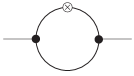
Figure 9: The two diagrams contributing to the flow of the 2-point function in a constant background field. The lines represent dressed propagators, $G_{\kappa}$. The cross represents an insertion of $\partial_{\kappa}R_{k}$. The vertices denoted by black dots are $\Gamma^{(3)}_{\kappa}$ and $\Gamma^{(4)}_{\kappa}$. When the background field vanishes, so does the diagram on the left.

When the external field vanishes, this equation simplifies greatly since then $\Gamma^{(3)}$ vanishes, and $\Gamma^{(2)}$ is diagonal :

$$\Gamma^{(2)}_{ab}(\kappa;q)=\delta_{ab}(q^{2}+\Sigma(\kappa;q),$$ (136)

which defines the self-energy $\Sigma$ (this $\Sigma$ differs from $\Sigma_{cl}$ introduced in sect. 3.2 by a factor $2m$; see e.g. eqs. (90) and (108)). We get then

$$\partial_{\kappa}\Gamma^{(2)}_{ab}(\kappa;p)=-{1\over 2}\int{d^{d}q\over(2\pi)^{d}}\,\partial_{\kappa}R_{\kappa}(q)\,G^{2}(\kappa;q)\,\Gamma^{(4)}_{abll}(\kappa;p,-p,q,-q),$$ (137)

where

$$G^{-1}(\kappa,q)=q^{2}+R_{\kappa}(q)+\Sigma(\kappa;q).$$ (138)

Similarly, the flow of the the 4-point function in vanishing field reads:

$$\partial_{\kappa}\Gamma^{(4)}_{abcd}(\kappa;p_{1},p_{2},p_{3},p_{4})=\int{d^{d}q\over(2\pi)^{d}}\,\partial_{\kappa}R_{k}(q^{2})\,G^{2}(\kappa;q)$$

$$\hskip 14.22636pt\times\left\{G(\kappa;q+p_{1}+p_{2})\Gamma^{(4)}_{abij}(\kappa;p_{1},p_{2},q,\cdot)\Gamma^{(4)}_{cdij}(\kappa;p_{3},p_{4},-q,\cdot)\right.$$

$$\hskip 22.76228pt+\,G(\kappa;q+p_{1}+p_{3})\Gamma^{(4)}_{acij}(\kappa;p_{1},p_{3},q,\cdot)\Gamma^{(4)}_{bdij}(\kappa;p_{2},p_{4},-q,\cdot)$$

$$\hskip 22.76228pt\left.+\,G(\kappa;q+p_{1}+p_{4})\Gamma^{(4)}_{adij}(\kappa;p_{1},p_{4},q,\cdot)\Gamma^{(4)}_{cbij}(\kappa;p_{3},p_{2},-q,\cdot)\right\}$$

$$\hskip 56.9055pt-\,{1\over 2}\int{d^{d}q\over(2\pi)^{d}}\partial_{\kappa}R_{\kappa}(q)G^{2}(\kappa;q)\Gamma^{(6)}_{abcdii}(\kappa;p_{1},p_{2},p_{3},p_{4},q,-q),$$

where we have used the abbreviated notation $\Gamma^{(4)}_{abij}(\kappa;p_{1},p_{2},q,-p_{1}-p_{2}-q)$ $\to$ $\Gamma^{(4)}_{abij}(\kappa;p_{1},p_{2},q,\cdot)$. The four contributions in the r.h.s. of eq. (4.1) are represented in the diagrams shown in figs. 10 and 11.

Eqs. (137) and (4.1) for the 2- and 4-point functions constitute the beginning of an infinite hierarchy of exact equations for the $n$-point functions, reminiscent of the Schwinger-Dyson hierarchy, with the flow equation for the $n$-point function involving all the $m$-point functions up to $m=n+2$. Clearly, solving this hierarchy requires approximations. A most natural approximation would rely on a truncation, in order to close the infinite hierarchy, as commonly done for instance in solving the Schwinger Dyson equations. For instance, one could ignore in eq. (4.1) the effect of the 6-point function on the flow of the 4-point function, arguing for instance that the 6-point function is perturbatively of order $u^{3}$. However such truncations prove to be not accurate enough for the present problem. Besides, the NPRG offers the possibility of exploring new approximation schemes that involve the entire functional $\Gamma[\phi]$ rather than the individual $n$-point functions. An example of such an approximation is provided by the derivative expansion described in the next section.

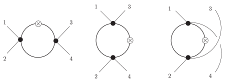
Figure 10: Diagrammatic illustration of the r.h.s. of the flow equation for the 4-point function, eq. (4.1): contribution of the 4-point functions (represented by black disks) in the three possible channels, from left to right. The crossed circle represents an insertion of $\partial_{\kappa}R_{\kappa}$, and the thick line a full propagator.

Figure 11: Diagrammatic illustration of the r.h.s. of the flow equation for the 4-point function, eq. (4.1): contribution of the 6-point function $\Gamma^{(6)}$ (represented by a black disk). The crossed circle represents an insertion of $\partial_{\kappa}R_{\kappa}$, and the thick line a full propagator.

4.2 The local potential approximation

The derivative expansion exploits the fact that the regulator in the flow equations (e.g. eqs. (137) or (4.1)) forces the loop momentum $q$ to be smaller than $\kappa$, i.e., only momenta $q\mathrel{\hbox to0.0pt{\raise 2.20013pt\hbox{$<$}\hss}{\lower 2.20013pt\hbox{$\sim$}}}\kappa$ contribute to the flow. Besides, in general, the regulator insures that all vertices are smooth functions of momenta. Then, in the calculation of the $n$-point functions at vanishing external momenta $p_{i}$, it is possible to expand the $n$-point functions in the r.h.s. of the flow equations in terms of $q^{2}/\kappa^{2}$, or equivalently in terms of the derivatives of the field.

In leading order, this procedure reduces to the so-called local potential approximation (LPA), which assumes that the effective action has the form:

$$\Gamma_{\kappa}^{LPA}[\phi]=\int d^{d}x\left\{{1\over 2}\partial_{\mu}\phi_{i}\partial_{\mu}\phi_{i}+V_{\kappa}(\rho)\right\},$$ (140)

where $\rho\equiv\phi_{i}\phi_{i}/2$. The derivative term here is simply the one appearing in the classical action, and $V_{\kappa}(\rho)$ is the effective potential. The exact flow equation for $V_{\kappa}$ is easily obtained by assuming that the field $\phi$ is constant in eq. (132). It reads:

$$\partial_{\kappa}V_{\kappa}(\rho)={1\over 2}\int{d^{d}q\over(2\pi)^{d}}\partial_{\kappa}R_{\kappa}(q)\left\{(N-1)G_{T}(\kappa;q)+G_{L}(\kappa;q)\right\},$$ (141)

where $G_{T}$ and $G_{L}$ are, respectively, the transverse and longitudinal components of the propagator:

$$G_{ij}(\kappa;q)=G_{T}(\kappa;q)\left(\delta_{ij}-{\phi_{i}\phi_{j}\over 2\rho}\right)+G_{L}(\kappa;q){\phi_{i}\phi_{j}\over 2\rho}.$$ (142)

By using the LPA effective action, eq.  (140), one gets

$$G_{T}^{-1}(\kappa;q) = q^{2}+V^{\prime}(\rho)+R_{k}(q),$$

$$G_{L}^{-1}(\kappa;q) = q^{2}+V^{\prime}(\rho)+2\rho V^{\prime\prime}(\rho)+R_{\kappa}(q),$$ (143)

with $V^{\prime}(\rho)=dV/d\rho$ and $V^{\prime\prime}(\rho)=d^{2}V/d\rho^{2}$.

The solution of the LPA is well documented in the literature (see e.g. Berges02 ; Canet02 ). In this section, we shall just, for illustrative purposes, solve approximately these equations, by keeping only a few terms in the expansion of the effective potential in powers of $\rho$ (thereby effectively implementing a truncation which ignores the effect of higher $n$-point functions on the flow). The derivatives of $V_{\kappa}(\rho)$ with respect to $\rho$ give the $n$-point functions at zero external momenta as a function of $\kappa$. We shall introduce a special notation for these $n$-point functions in vanishing external field:

$$m_{\kappa}^{2}\equiv\left.{dV_{\kappa}\over d\rho}\right|_{\rho=0},\hskip 28.45274ptg_{\kappa}\equiv\left.{d^{2}V_{\kappa}\over d\rho^{2}}\right|_{\rho=0},\hskip 28.45274pth_{\kappa}\equiv\left.{d^{3}V_{\kappa}\over d\rho^{3}}\right|_{\rho=0}.$$ (144)

The equations for these $n$-point functions are obtained by differentiating once and twice eq. (141) with respect to $\rho$, then setting $\rho=0$, and using the definitions in eq. (144). One gets, respectively:

$$\kappa\partial_{\kappa}m_{\kappa}^{2}=-{(N+2)\over 2}g_{\kappa}I_{d}^{(2)},$$ (145)

and

$$\kappa\partial_{\kappa}g_{\kappa}=(N+8)g_{\kappa}^{2}I_{d}^{(3)}(\kappa)-{1\over 2}(N+4)\;h_{\kappa}I_{d}^{(2)}(\kappa),$$ (146)

where we have defined

$$I_{d}^{(n)}(\kappa) \equiv \int{d^{d}q\over(2\pi)^{d}}\kappa\partial_{\kappa}R_{\kappa}(q^{2})G^{n}(\kappa;q)$$ (147)

$$= 2K_{d}{\kappa^{d+2}\over(\kappa^{2}+m^{2}_{\kappa})^{n}},$$

the explicit form in the second line being obtained for the regulator (128) and

$$K_{d}^{-1}\equiv\;2^{d-1}\;\pi^{d/2}\;d\;\Gamma(d/2).$$ (148)

We have used the fact that for vanishing external field, the propagator is diagonal and $\Sigma(\kappa,q)=m_{\kappa}^{2}$ (see Eqs. (136) and (138)). Eqs. (145) and (146) are solved starting from the initial condition at $\kappa=\Lambda$:

$$m_{\Lambda}^{2}=r\qquad g_{\Lambda}={u\over 3}.$$ (149)

In order to factor out the large variations which arise when $\kappa$ varies from the microscopic scale $\Lambda$ to the physical scale $\kappa=0$, and also to exhibit the fixed point structure, it is convenient to isolate the explicit scale factors and to define dimensionless quantities:

$$m_{\kappa}^{2}\equiv\kappa^{2}\,\hat{m}_{\kappa}^{2},\hskip 28.45274ptg_{\kappa}\equiv K_{d}^{-1}\kappa^{4-d}\,\hat{g}_{\kappa},\hskip 28.45274pth_{\kappa}\equiv K_{d}^{-2}\kappa^{6-2d}\,\hat{h}_{\kappa}.$$ (150)

If one assumes that $\hat{m}_{\kappa}\ll 1$, and ignore the contribution of $h_{\kappa}$, then the equation for $\hat{g}_{\kappa}$ becomes:

$$\kappa{d\hat{g}_{\kappa}\over d\kappa}=(d-4)\,\hat{g}_{\kappa}+2(N+8)\,\hat{g}_{\kappa}^{2},\$$ (151)

and can be solved explicitly:

$$\hat{g}_{\kappa}={\hat{g}^{*}\over 1+\left({\kappa\over\kappa_{c}}\right)^{4-d}},$$ (152)

where $\hat{g}^{*}$ is the value of $\hat{g}$ at the IR fixed point, $\hat{g}^{*}=(4-d)/{(2(N+8))}$, and $\kappa_{c}$ the value of $\kappa$ for which $\hat{g}_{\kappa}=\hat{g}^{*}/2$. We have:

$$\left({\kappa_{c}\over\Lambda}\right)^{d-4}={\hat{g}^{*}-\hat{g}_{\Lambda}\over\hat{g}_{\Lambda}}\approx{\hat{g}^{*}\over\hat{g}_{\Lambda}}.$$ (153)

where the last approximate equality holds if $\hat{g}^{*}\gg\hat{g}_{\Lambda}$. In this regime, one recovers the qualitative feature already discussed in the previous lecture: there exists a well defined scale $\kappa_{c}\ll\Lambda$, $\kappa_{c}^{4-d}=uK_{d}/(3\hat{g}^{*})$, that separates the scaling region, dominated by the IR fixed point, where $\hat{g}=\hat{g}^{*}$, from the perturbative region, dominated by the UV fixed point $\hat{g}=0$ (when $\kappa\gg\kappa_{c}$, one can expand $\hat{g}_{\kappa}$ in powers of $\kappa_{c}/\kappa$; in leading order $g_{\kappa}=(u/3)(1-(\kappa_{c}/\kappa)^{4-d})$).

The local potential approximation, or a refined version of it, enters in an essential way in the approximation scheme that we have developed in order to calculate $\Sigma(p)$. Further insight can be gained by studying the $n$-point functions in the large $N$ limit, to which we now turn.

4.3 Correlation functions in the large $N$ limit

The LPA, as well as the higher orders of the derivative expansion, give accurate results for the correlation functions and their derivatives only at zero external momenta. In order to get insight into the effect of non vanishing external momenta we consider now the correlation functions in the large $N$ limit (at fixed $uN$) Ellwanger94 ; Tetradis95 ; D'Attanasio97 ; Blaizot:2005xy .

For vanishing field, the inverse propagator has the same form as in the LPA, eq. (138), where the running mass $m_{\kappa}$ is here given by a gap equation

$$m_{\kappa}^{2}=r+{Nu\over 6}\int{d^{d}q\over(2\pi)^{d}}\,(G(\kappa;q)-G(\Lambda;q)).$$ (154)

Figure 12: Diagrams representing the contribution to $\Gamma_{1234}^{(4)}(\kappa;p_{1},p_{2},p_{3},p_{4})$ in the first channel of eq. (4.3). This diagram represents also a typical contribution to the function $g_{\kappa}(p)$ of eq. (156). External momenta are counted as incoming momenta, so that $p_{1}+p_{2}$ flows into the bubble chain, and $p_{3}+p_{4}=-(p_{1}+p_{2})$.

The 4-point function has the following structure:

$$\Gamma_{1234}^{(4)}(\kappa;p_{1},p_{2},p_{3},p_{4})=$$

$$\qquad\delta_{12}\delta_{34}g_{\kappa}(p_{1}+p_{2})+\delta_{13}\delta_{24}g_{\kappa}(p_{1}+p_{3})+\delta_{14}\delta_{23}g_{\kappa}(p_{1}+p_{4}),$$

where $g_{\kappa}(p)$ is given by

$$g_{\kappa}(p)={u\over 3}{1\over 1+{Nu\over 6}B_{d}(\kappa;p)},$$ (156)

with

$$B_{d}(\kappa;p)\equiv\int{d^{d}q\over(2\pi)^{d}}\,G(\kappa;q)G(\kappa;p+q).$$ (157)

Finally the 6-point function $\Gamma_{1234mm}^{(6)}(\kappa;p_{1},p_{2},p_{3},p_{4},q,-q)$ (summation over repeated indices is understood) is of the form

$${1\over N}\Gamma_{1234mm}^{(6)}(\kappa;p_{1},p_{2},p_{3},p_{4},q,-q)$$

$$=h_{\kappa}(p_{1}+p_{2})\delta_{12}\delta_{34}+h_{\kappa}(p_{1}+p_{3})\delta_{13}\delta_{24}+h_{\kappa}(p_{1}+p_{4})\delta_{14}\delta_{23},$$ (158)

with

$$h_{\kappa}(p)=Ng_{\kappa}(0)g^{2}_{\kappa}(p)\int{d^{d}q^{\prime}\over(2\pi)^{d}}G^{2}(\kappa;q^{\prime})G(\kappa;q^{\prime}+p).$$ (159)

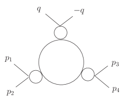
Figure 13: Diagrams representing the contribution to $\Gamma_{1234mm}^{(6)}(\kappa;p_{1},p_{2},p_{3},p_{4},q,-q)$ in eq. (4.3). The small circles represent the function $g_{\kappa}(p)$ with $p$ the momentum flowing through the vertex. The convention for momenta is as in Fig. 12.

Note that a single function, $g_{\kappa}(p)$, suffices to calculate all the $n$-point functions in the large $N$ limit. These can be obtained in a straightforward fashion by calculating the corresponding Feynman diagrams with a regulator (see Figs. 12 and 13). It is however easy to verify that the various $n$-point functions that we have just written are indeed solutions of the flow equations in the large $N$ limit.

To this aim, one notes first that eq. (137) reduces to an equation for the running mass:

$$\partial_{\kappa}m_{\kappa}^{2}=-{1\over 2}Ng_{\kappa}(0)\int{d^{d}q\over(2\pi)^{d}}\partial_{\kappa}R_{\kappa}(q)G^{2}(\kappa;q),$$ (160)

and using eq. (156), it is easy to check that this equation is equivalent to the gap equation, eq. (154).

Next, we observe that in the large $N$ limit, a single channel effectively contributes in eq. (4.1) for the $4$-point function; one can then use the following identity in this limit:

$$\Gamma^{(4)}_{12ij}(\kappa;p_{1},p_{2},q,\!-\!q\!-\!p_{1}\!-\!p_{2})\Gamma^{(4)}_{34ij}(\kappa;p_{3},p_{4},\!-\!q,q\!-\!p_{3}\!-\!p_{4})$$

$$\qquad\qquad=Ng^{2}_{\kappa}(p_{1}+p_{2})\delta_{12}\delta_{34},$$ (161)

together with eq. (4.3) for $\Gamma^{(6)}$, and one obtains:

$$\kappa\partial_{\kappa}g_{\kappa}(p)=Ng_{\kappa}^{2}(p)J^{(3)}_{d}(\kappa;p)-{N\over 2}h_{\kappa}(p)I^{(2)}_{d}(\kappa),$$ (162)

where the function $I^{(2)}_{d}(\kappa)$ is that defined in eq. (147), with $n=2$ . The function $J_{d}^{(3)}(\kappa;p)$ is obtained from the general definition

$$J_{d}^{(n)}(\kappa;p)\equiv\int{d^{d}q\over(2\pi)^{d}}\kappa\partial_{\kappa}R_{\kappa}(q)G^{n-1}(\kappa;q)G(\kappa;p+q).$$ (163)

Note that $J_{d}^{(n)}(\kappa;p=0)=I_{d}^{(n)}(\kappa)$.

At this point we remark that the flow equation for $g_{\kappa}(p)$ can also be obtained directly from the explicit expression (156), in the form:

$$\partial_{\kappa}g_{\kappa}(p)=-{N\over 2}g^{2}_{\kappa}(p)\partial_{\kappa}\int{d^{d}q\over(2\pi)^{d}}G(\kappa;q)G(\kappa;q+p).$$ (164)

It is then straightforward to verify, using eqs. (160) and (159) that eqs. (162) and (164) are indeed equivalent. The first term in eq. (162) comes from the derivative of the cut-off function in the propagators in eq. (164), while the second term, which involves the 6-point vertex, comes from the derivative of the running mass in the propagators.

Note that eqs. (160) for $m_{\kappa}$ and (162) for $g_{\kappa}(p=0)$ become identical respectively to eqs. (145) and (146) of the LPA in the large $N$ limit, a well know property D'Attanasio97 .

Let us now analyze characteristic features of the function $g_{\kappa}(p)$. For simplicity we specialize for the rest of this subsection to $d=3$. Furthermore, for the purpose of the present, qualitative, discussion, one may assume $m_{\kappa}=0$. This allows us to obtain easily $g_{\kappa}(p)$ from eq. (156) in the two limiting cases $p=0$ and $\kappa=0$. In the first case, we have

$$g_{\kappa}(0)={u\over 3}{1\over 1+{uN\over 9\pi^{2}}{1\over\kappa}}.$$ (165)

This is identical to eq. (152), with here $\hat{g}^{*}=1/(2N)$ and $\kappa_{c}=Nu/9\pi^{2}$ . In the other case, we have

$$g_{\kappa=0}(p)={u\over 3}{1\over 1+{uN\over 48}{1\over p}}={u\over 3}{p\over p+p_{c}},$$ (166)

with $p_{c}\equiv{uN}/{48}$.

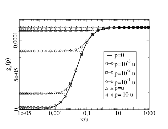
Figure 14: The function $g_{\kappa}(p)$ (in units of $\Lambda$) obtained from a complete numerical solution of eqs. (160) and (162), as a function of $\kappa/u$ (in a logarithmic scale) for five values of $p$: from bottom to top, $p/u=0.001,0.01,0.1,1$ and $10$. The envelope corresponds to $p=0$. This figure illustrates the decoupling of modes: for each value of $p$, the flow stops when $\kappa\mathrel{\hbox to0.0pt{\raise 2.20013pt\hbox{$<$}\hss}{\lower 2.20013pt\hbox{$\sim$}}}\alpha p$. The various horizontal asymptotes (dotted llines) correspond to the single value $\alpha=0.54$. From Ref. Blaizot:2005wd .

One sees on eqs. (165) and (166) that the dependence on $p$ of $g_{\kappa=0}(p)$ is quite similar to the dependence on $\kappa$ of $g_{\kappa}(p=0)$. In particular both quantities vanish linearly as $\kappa\to 0$ or $p\to 0$, respectively. The result of the complete (numerical) calculation, including the effect of the running mass ( i.e., solving the gap equation (154) and calculating $g_{\kappa}(p)$ from eq. (156)), can in fact be quite well represented (to within a few percents) for arbitrary $p$ and $\kappa$ by the following approximate formula

$$g_{\kappa}(p)\approx{u\over 3}{X\over 1+X}\qquad X\equiv{\kappa\over\kappa_{c}}+{p\over p_{c}}.$$ (167)

This simple expression shows that $p$, when it is non vanishing, plays the same role as $\kappa$ as an infrared regulator. In particular, at fixed $p$, the flow of $g_{\kappa}(p)$ stops when $X$ becomes independent of $\kappa$, i.e., when $\kappa\mathrel{\hbox to0.0pt{\raise 2.20013pt\hbox{$<$}\hss}{\lower 2.20013pt\hbox{$\sim$}}}p(\kappa_{c}/p_{c})$, with $\kappa_{c}/p_{c}=16/3\pi^{2}\approx 0.54$. This important property of decoupling of the short wavelength modes is illustrated in Fig. 14. As shown by this figure, and also by the expression (167), the momentum dependence of the 4-point function can be obtained from its cut-off dependence at zero momentum. In fact Fig. 14 suggests that, to a very good approximation, there exists a parameter $\alpha$ such that $g(\kappa;p)\approx g(\kappa;0)$ when $\kappa>\alpha p$, and $g(\kappa;p)\approx g(\kappa=\alpha p;0)$ when $\kappa<\alpha p$. From the discussion above, one expects $\alpha\approx\kappa_{c}/p_{c}=16/3\pi^{2}\approx 0.54$, which is indeed in agreement with the analysis in Fig. 14.

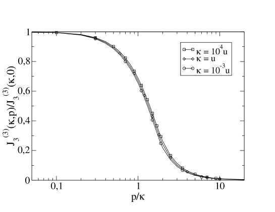
Figure 15: The function $J_{3}^{(3)}(\kappa;p)/I_{3}^{(3)}(\kappa)$ as a function of $p/\kappa$ (in a logarithmic scale), for different values of $\kappa$: $\kappa=10^{-3}u$ (circles), $\kappa=u$ (diamonds) and $\kappa=10^{4}u$ (squares). From Ref. Blaizot:2005wd .

The decoupling of modes can also be visualized in Fig. 15. The $p$-dependence of $J_{d}^{(n)}(\kappa;p)$ (eq. (163)) shown in this figure is relatively simple: when $p\ll\kappa$, $J_{d}^{(n)}(\kappa;p)\simeq I_{d}^{(n)}(\kappa)$; when $p\gg\kappa$, $J_{d}^{(n)}(\kappa;p)$ vanishes as $1/p^{2}$. On a logarithmic scale the transition between these two regimes occurs rapidly at momentum $p\sim\kappa$, as illustrated on Fig. 15. A similar analysis can be made for the contribtution of the 6-point function in eq. (162), and one can show that the ratio of the $p$-dependence of the second term in the right hand side (the one proportional to $h_{\kappa}$) is, whenever it is significant, proportional to that of the first term, the proportionality coefficient being a function of $\kappa$ only.

All this suggests that one can rewrite eq. (162) for $g_{\kappa}(p)$ as follows:

$$\partial_{\kappa}g_{\kappa}(p)\approx Ng_{\kappa}^{2}(p)\Theta(1-{\alpha^{2}p^{2}\over\kappa^{2}})I^{(3)}_{d}(\kappa)(1-F_{\kappa}),$$ (168)

where $\alpha$ is a parameter of order unity. The $\Theta$-function ensures that the flow exists only when $\kappa>\alpha p$, and stops for smaller values of $\kappa$.

These approximations, together with another one that we shall discuss more thoroughly in the next section have been used in order to construct approximate flow equations in Refs. Blaizot:2005wd ; Blaizot:2006vr .

4.4 Beyond the derivative expansion

The arguments on which the derivative expansion is based can be generalized in order to set up a much more powerful approximation scheme Blaizot:2005xy that we now briefly present. This scheme allows us to obtain the momentum dependence of the $n$-point function with a single approximation.

We observe that: i) the momentum $q$ circulating in the loop integral of a flow equation is limited by $\kappa$; ii) the smoothness of the $n$-point functions allows us to make an expansion in powers of $q^{2}/\kappa^{2}$, independently of the value of the external momenta $p$. Now, a typical $n$-point function entering a flow equation is of the from $\Gamma^{(n)}_{\kappa}(p_{1},p_{2},...,p_{n-1}+q,p_{n}-q;\phi)$, where $q$ is the loop momentum. The proposed approximation scheme, in its leading order, consists in neglecting the $q$-dependence of such vertex functions:

$$\Gamma^{(n)}_{\kappa}(p_{1},p_{2},...,p_{n-1}+q,p_{n}-q;\phi)\sim\Gamma^{(n)}_{\kappa}(p_{1},p_{2},...,p_{n-1},p_{n};\phi).$$ (169)

Note that this approximation is a priori well justified. Indeed, when all the external momenta vanish $p_{i}=0$, eq. (169) is the basis of the LPA which, as stated above, is a good approximation. When the external momenta $p_{i}$ begin to grow, the approximation in eq. (169) becomes better and better, and it is trivial when all momenta are much larger than $\kappa$. With this approximation, eq. (137) becomes (for simplicity we set here $N=1$):

$$\partial_{\kappa}\Gamma_{\kappa}^{(2)}(p,-p;\phi) = \int{d^{d}q\over(2\pi)^{d}}\partial_{\kappa}R_{k}(q^{2})\left\{G_{\kappa}(q^{2};\phi)\Gamma_{\kappa}^{(3)}(p,0,-p;\phi)\right.$$ (170)

$$\times G_{\kappa}((q+p)^{2};\phi)\Gamma_{\kappa}^{(3)}(-p,p,0;\phi)G_{\kappa}(q^{2};\phi)$$

$$\left.-{1\over 2}G_{\kappa}(q^{2};\phi)\Gamma_{\kappa}^{(4)}(p,-p,0,0;\phi)G_{\kappa}(q^{2};\phi)\right\}.$$

Now comes the second ingredient of the approximation scheme, which exploits the advantage of working with a non vanishing background field: vertices evaluated at zero external momenta can be obtained as derivatives of vertex functions with a smaller number of legs:

$$\Gamma_{\kappa}^{(n+1)}(p_{1},p_{2},...,p_{n},0;\phi)={\partial\Gamma_{\kappa}^{(n)}(p_{1},p_{2},...p_{n};\phi)\over\partial\phi}.$$ (171)

By exploiting eq. (171), one easily transforms eq. (170) into a closed equation (recall that $G_{\kappa}$ and $\Gamma_{\kappa}^{(2)}$ are related by eq. (133)):

$$\partial_{\kappa}\Gamma_{\kappa}^{(2)}(p^{2};\phi)=\int{d^{d}q\over(2\pi)^{d}}\,\partial_{\kappa}R_{\kappa}(q^{2})\;G^{2}_{\kappa}(q^{2};\phi)$$

$$\times\left\{\left({\partial\Gamma_{\kappa}^{(2)}(p,-p;\phi)\over\partial\phi}\right)^{2}G_{\kappa}((p+q)^{2};\phi)\;-\;{1\over 2}{\partial^{2}\Gamma_{\kappa}^{(2)}(p,-p;\phi)\over\partial\phi^{2}}\right\}.$$ (172)

Note the similarity of this equation with eq. (141): both are closed equations, the vertices appearing in the r.h.s. being expressed as derivatives of the function in the l.h.s..

The approximation scheme presented here is similar to that used in Blaizot:2005wd ; Blaizot:2006vr . There also the momentum dependence of the vertices was neglected in the leading order. However further approximations were needed in order to close the hierarchy. The progress realized here is to bypass these extra approximations by working in a constant background field.

The resulting equations can be solved with a numerical effort comparable to that involved in solving the equations of the derivative expansion. The preliminary results obtained so far are encouraging Blaizot:2006ak .

4.5 Calculation of $\Delta\langle\varphi^{2}\rangle$

We come now to the conclusion of these lectures, where results concerning the numerical value of $c$ obtained with the NPRG will be presented.

The approximation developed in Blaizot:2004qa ; Blaizot:2005wd ; Blaizot:2006vr is based on an iteration scheme, where one starts by building approximate equations for the $n$-point functions, that are then solved exactly. To give a flavor of this method, consider more specifically the equation (4.1) for the 4-point function. An approximate flow equation is obtained with the following three approximations:

Our first approximation is that discussed in sect. 4.4: we ignore the $q$ dependence of the vertices in the flow equation, i.e., we set $q=0$ in the vertices $\Gamma^{(4)}$ and $\Gamma^{(6)}$ and factor them out of the integral in the r.h.s. of eq. (4.1). The second approximation concerns the propagators in the flow equation, for which we make the replacements:

$$G(p+q)\longrightarrow G_{LPA^{\prime}}(q)\,\Theta\left(1-{\alpha^{2}p^{2}\over\kappa^{2}}\right)$$ (173)

where $\alpha$ is an adjustable parameter. A motivation for this approximation may be obtained from the analysis of the $n$-point function presented in sect. 4.3 (see eq. (168) and Fig. 15). This approximation introduces a dependence of the results on the value of $\alpha$. The third approximation concerns the function $\Gamma^{(6)}$ for which we use an ansatz inspired by the expressions of the various $n$-point functions in the large $N$ limit (see again the discussion at the end of sect. 4.3): one assumes that the contribution of $\Gamma^{(6)}$ to the r.h.s. of eq. (4.1) is proportional to that of the other terms, the proportionality coefficient $F_{\kappa}$ being only a function of $\kappa$. The same proportionality also holds in the LPA regime, which allows us to use the LPA to determine $F_{\kappa}$.

These three approximations result then in the following approximate equation for $\Gamma^{(4)}$:

$$\partial_{\kappa}\Gamma^{(4)}_{ijkl}(\kappa;p_{1},p_{2},p_{3},p_{4})=I^{(3)}_{\kappa}(0)\,(1-F_{\kappa})$$

$$\hskip 2.84544pt\times\left\{\Theta\!\!\left(\kappa^{2}-\alpha^{2}{(p_{1}+p_{2})^{2}})\right)\Gamma^{(4)}_{ijmn}(\kappa;p_{1},p_{2},0,-p_{1}-p_{2})\right.$$

$$\hskip 28.45274pt\left.\times\Gamma^{(4)}_{klnm}(\kappa;p_{3},p_{4},-p_{3}-p_{4},0)+{\rm permutations}\right\}.$$ (174)

This equation can be solved analytically in terms of the solution of the LPA (actually a refined version of it). This is done by steps, starting form the momentum domain $\alpha^{2}(p_{1}+p_{2})^{2},\alpha^{2}(p_{1}+p_{3})^{2},\alpha^{2}(p_{1}+p_{4})^{2}\leq\kappa^{2}$, where it can be verified that the solution is that of the LPA itself. The solution of this equation is then inserted in eq. (137) for the 2-point function and leads to the leading order determination of $\Sigma(p)$. The scheme is improved through an iteration procedure. At next-to-leading order, one improves $\Gamma^{(4)}$ by establishing an approximate equation for $\Gamma^{(6)}$. The solution of this equation is then used in eq. (4.1) for $\Gamma^{(4)}$, and the resulting $\Gamma^{(4)}$ is used in turn in eq. (137) to get $\Sigma$ at next-to-leading order.

$c$	$N=1$	$N=2$	$N=3$	$N=4$	$N=10$	$N=40$	$N=\infty$
lattice latt2		$1.32\pm 0.02$
lattice latt1		$1.29\pm 0.05$
lattice latt3	$1.09\pm 0.09$			$1.60\pm 0.10$
7-loops Kastening:2003iu	$1.07\pm 0.10$	$1.27\pm 0.10$	$1.43\pm 0.11$	$1.54\pm 0.11$
large $N$ BigN							$c=2.33$
NPRG	1.11	1.30	1.45	1.57	1.91	2.12

Table 1: Summary of available results for the coefficient $c$. The last line contains the results obtained in Blaizot:2006vr .

The results obtained with this method for the value of $c$ are reported in Table 1 and Fig. 16 for various values of $N$ for which results have been obtained with other techniques, either the lattice technique latt2 ; latt1 ; latt3 , or variationally improved 7-loops perturtbative calculations Kastening:2003iu (other optimized perturbative calculations have also been recently performed, and are in agreement with those quoted here; see souza ; Kneur04 ). The results reported in Table 1 have been obtained with an improved next-to-leading order calculation where, among other things, the parameter $\alpha$ of eq. (173) has been fixed by a principle of minimum sensitivity (see Blaizot:2006vr for details). A recent (approximate) calculation along the lines described in sect. 4.4 yields, for $N=1$, the value $c=1.2$ Blaizot:2006ak . Let me also mention the result $c=1.23$ obtained, for $N=2$ in Ref. Ledowski03 ; however, as discussed in Blaizot:2006vr it is difficult to gauge the quality of the approximation made in Ledowski03 .

For $N\leq 4$, where we can compare with other results, the values of $c$ obtained with the present improved NLO calculation are in excellent agreement with those obtained from lattice and “7-loops” calculations. What happens at large values of $N$ deserves a special discussion. As seen in Fig. 16 the curve showing the improved leading order results extrapolates when $N\to\infty$ to a value that is about $4\%$ below the known exact result BigN . A direct calculation at very large values of $N$ is difficult in the present approach for numerical reasons: since the coefficient $c$ represents in effect an order $1/N$ correction (see BigN ), it is necessary to insure the cancellation of the large, order $N$, contributions to the self-energy, in order to extract the value of $c$. This is numerically demanding when $N\mathrel{\hbox to0.0pt{\raise 2.20013pt\hbox{$>$}\hss}{\lower 2.20013pt\hbox{$\sim$}}}100$. Fig. 16 also reveals an intriguing feature: there seems to be no natural way to reconcile the present results, and for this matter the results from lattice calculations or 7-loop calculations, with the calculation of the $1/N$ correction presented in Ref. Arnold:2000ef : the dependence in $1/N$ of our results, be they obtained from the direct NLO or the improved NLO, appear to be incompatible with the slope predicted in Ref. Arnold:2000ef for the $1/N$ expansion.

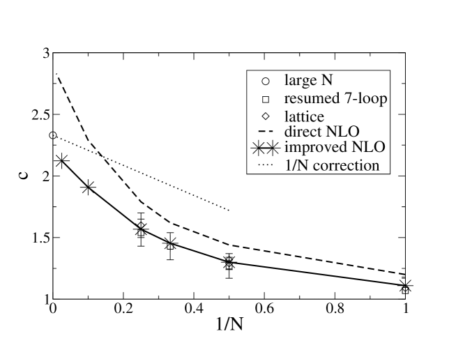
Figure 16: The coefficient $c$ (obtained with the fastest apparent convergence procedure) as a function of $1/N$. Our NLO results, are compared with results obtained with other methods: lattice latt2 ; latt1 ; latt3 (diamonds) and 7-loops perturbation theory Kastening:2003iu (squares), all of them with their corresponding error bars, together with the $N\to\infty$ result BigN (circle), and the extrapolation following the $1/N$ correction calculated in Ref. Arnold:2000ef . From Ref. Blaizot:2006vr .

Acknowledgements. Most of the material of these lectures is drawn from work done in a most enjoyable collaboration with several people during these last years: G. Baym, F. Laloë, M. Holzmann, R. Mendez-Galain, D. Vautherin, N. Wschebor, J. Zinn-Justin. I would also like to express my gratitude to Achim Schwenk for insisting on having these lecture notes….and putting such a high cut-off on his patience as he waited for them.

References

- (1) L. Pitaevskii and S. Stringari, Bose-Eisntein condensation, Oxford University Press, UK, 2003.
- (2) C.J. Pethick and H. Smith, Bose-Eisntein condensation in dilute gases, Cambridge University Press, UK, 2003.
- (3) F. Dalfovo, S. Giorgini, S. Stringari, and L. Pitaevskii, Rev. Mod. Phys. 71, 463 (1999).
- (4) A. J. Legget. Bose-einstein condensation in the alkali gases: Some fundamental concepts. Rev. Mod. Phys., 73:307, 2001.
- (5) J. O. Andersen, Rev. Mod. Phys. 76 (2004) 599
- (6) G. Baym, J-P. Blaizot, M. Holzmann, F. Laloë and D. Vautherin, Phys. Rev. Lett. 83, 1703 (1999).
- (7) G. Baym, J-P. Blaizot and J. Zinn-Justin, Europhys. Lett. 49, 150 (2000).
- (8) G. Baym, J-P. Blaizot, M. Holzmann, F. Laloë and D. Vautherin, Eur. Phys. J. B 24 (2001) 107.
- (9) M. Holzmann, G. Baym, J.-P. Blaizot, and F. Laloë, Phys. Rev. Lett. 87, 120403 (2001).
- (10) M. Holzmann, J.N. Fuchs, G. Baym, J.-P. Blaizot, and F. Laloë, Comptes Rendus Physique 5 (2004)21.
- (11) J. P. Blaizot, R. Mendez Galain and N. Wschebor, Europhys. Lett., 72 (5), 705-711 (2005).
- (12) J. P. Blaizot, R. Mendez-Galain and N. Wschebor, Phys. Rev. E74 (2006) 051116.
- (13) J. P. Blaizot, R. Mendez-Galain and N. Wschebor, Phys. Rev. E74 (2006) 051117.
- (14) J. P. Blaizot, R. Mendez Galain and N. Wschebor, Phys. Lett. B 632, 571 (2006).
- (15) J. P. Blaizot, R. Mendez-Galain and N. Wschebor, arXiv:hep-th/0605252.
- (16) R.M. Ziff, G.E. Uhlenbeck and M. Kac, Phys. Rep. 32 (1977) 169.
- (17) M. Holzmann, G. Baym, J.-P. Blaizot, F. Laloë, PNAS 2007 104: 1476-1481.
- (18) S. Giorgini, L. Pitaevskii and S. Stringari, Phys. Rev. A54 (1996) 4633.
- (19) T. Schafer, arXiv:nucl-th/0609075.
- (20) D. B. Kaplan, arXiv:nucl-th/0510023.
- (21) E. Braaten and A. Nieto, arXiv:hep-th/9609047.
- (22) E. Braaten and A. Nieto, arXiv:cond-mat/9707199.
- (23) E. Braaten, H. W. Hammer and S. Hermans, Phys. Rev. A 63 (2001) 063609.
- (24) T. Toyoda, Annals of Physics N.Y. 141, 154 (1982).
- (25) A.L. Fetter and J.D. Walecka, Quantum theory of many-particle systems, McGraw-Hill (1971), 28.
- (26) G. Baym and G. Grinstein, Phys. Rev. D15, 2897 (1977).
- (27) L.P. Kadanoff and G. Baym, Quantum statistical mechanics, Benjamin (1962).
- (28) A. A. Abrikosov, L.P. Gorkov, and I.E. Dzyaloshinski, Methods of quantum field theory in statistical physics, Prentice Hall (1963).
- (29) J.P. Blaizot and G. Ripka, Quantum theory of finite systems, MIT Press (1986).
- (30) A.Z. Patashinskii and V.L. Pokrovskii, Fluctuation theory of phase transitions, Pergamon Press (1979).
- (31) P. Ginsparg, Nucl. Phys. B170 (1980) 388.
- (32) T. Appelquist and R.D. Pisarski, Phys. Rev. D23 (1981) 2305.
- (33) S. Nadkarni, Phys. Rev. D27 (1983) 917; Phys. Rev. D38 (1988) 3287.
- (34) P. Arnold and B. Tomasik, Phys. Rev. A64 (2001) 053609.
- (35) M. Moshe and J. Zinn-Justin, Phys. Rept. 385, 69 (2003)
- (36) P. Arnold and B. Tomasik, Phys. Rev. A 62 (2000) 063604.
- (37) J. Zinn-Justin, Quantum field theory and critical phenomena, Int. Ser. Monogr. Phys. 113, 1 (2002).
- (38) P. Arnold and G. Moore, Phys. Rev. Lett. 87, 120401 (2001); Phys. Rev. E64, 066113 (2001).
- (39) V.A. Kashurnikov, N. V. Prokof’ev, and B. V. Svistunov, Phys. Rev. Lett. 87, 160601 (2001); Phys. Rev. Lett. 87, 120402 (2001).
- (40) J.-L. Kneur, A. Neveu, M. B. Pinto, Phys. Rev. A69, 053624 (2004).
- (41) F. de Souza Cruz, M.B. Pinto, and R.O. Ramos, Phys. Rev. B64, 014515 (2001); Phys. Rev. A 65, 053613 (2002).
- (42) B. Kastening, Phys. Rev. A 68, 061601 (R) (2003); Phys. Rev. A 69, 043613 (2004).
- (43) P. Arnold, G. D. Moore and B. Tomasik, Phys. Rev. A 65 (2002) 013606
- (44) C.Wetterich, Phys. Lett., B301, 90 (1993).
- (45) U.Ellwanger, Z.Phys., C58, 619 (1993).
- (46) N. Tetradis and C. Wetterich, Nucl. Phys. B 422, 541 (1994).
- (47) T.R.Morris, Int. J. Mod. Phys., A9, 2411 (1994).
- (48) T.R.Morris, Phys. Lett. B329, 241 (1994).
- (49) C. Bagnuls and C. Bervillier, Phys. Rept. 348, 91 (2001).
- (50) J. Berges, N. Tetradis and C. Wetterich, Phys. Rept. 363, 223–386 (2002).
- (51) B. Delamotte, D. Mouhanna, M. Tissier, Phys. Rev. B69, 134413 (2004); L. Canet and B. Delamotte, cond-matt/0412205.
- (52) H. Gies, arXiv:hep-ph/0611146.
- (53) M. Bijlsma and H.T.C. Stoof, Phys. Rev. A54, 5085 (1996).
- (54) J. O. Andersen and M. Strickland, arXiv:cond-mat/9808346.
- (55) J. O. Andersen and M. Strickland, Phys. Rev. A 60 (1999) 1442.
- (56) R.D.Ball, P.E.Haagensen, J.I.Latorre and E. Moreno, Phys. Lett., B347, 80 (1995).
- (57) J.Comellas, Nucl. Phys., B509, 662 (1998).
- (58) D.Litim, Phys. Lett. B486, 92 (2000); Phys. Rev. D64, 105007 (2001); Nucl. Phys. B631, 128 (2002); Int.J.Mod.Phys. A16, 2081 (2001).
- (59) L.Canet, B.Delamotte, D.Mouhanna and J.Vidal, Phys. Rev. D67, 065004 (2003).
- (60) U. Ellwanger and C. Wetterich, Nucl. Phys. B423, 137(1994).
- (61) N. Tetradis and D. F. Litim, Nucl. Phys. B464, 492–511 (1996).
- (62) M. D’Attanasio and T. R. Morris, Phys. Lett. B409, 363–370 (1997).
- (63) X. Sun, Phys. Rev. E67, 066702 (2003).
- (64) S.Ledowski, N. Hasselmann and P. Kopietz, Phys. Rev. A 69, 061601(R) (2004); Phys. Rev. A 70, 063621 (2004).