Phase transition in the scalar noise model of collective motion in three dimensions

Abstract

We consider disorder-order phase transitions in the three-dimensional version of the scalar noise model (SNM) of flocking. Our results are analogous to those found for the two-dimensional case nagy and vicsek . For small velocity ($v\leq 0.1$) a continuous, second-order phase transition is observable, with the diffusion of nearby particles being isotropic. By increasing the particle velocities the phase transition changes to first order, and the diffusion becomes anisotropic. The first-order transition in the latter case is probably caused by the interplay between anisotropic diffusion and periodic boundary conditions, leading to a boundary condition dependent symmetry breaking of the solutions.

1 Introduction

The collective motion of animals is a fascinating phenomenon, resulting from the occasionally very simple interactions between individuals. Self-propelled particle (SPP) models vicsek ; czirok ; csahok ; tonertu1 ; tonertu2 ; tonertu3 ; czirok_3d ; gregoire play a crucial role in understanding of the dynamics of these biological systems animal , be them bird flocks birds , fish schools fish , insect swarms insect or bacteria aggregates bacteria . A common feature of these groups is the onset of collective motion without a leader.

The two dimensional scalar noise model (SNM) is able to reproduce some fundamental properties of these collective motions. In spite of its simplicity, the SNM reproduces the emergence of cooperative motion from a disordered phase in the absence a ”leader” particle vicsek . The velocity of particles $v$ provides a control parameter which switches between SPP behaviour ($v>0$) and equilibrium type models ($v=0$). It means that there is a kinetic phase transition between a disordered state and an ordered state; in the latter one most of the particles move nearly in the same direction.

The original model of Ref. vicsek assumes a constant velocity $v$ for each particle. The particles in every time step adopt the average velocity of particles within a neighbourhood radius $R$. Besides, there is a random noise, an angle added to the direction of the velocity in order to involve realistic noise elements. However, the dynamic properties of this system, being subject to random velocity fluctuations, are likely to depend strongly on the dimensionality of the space, as it was discussed in Ref. czirok_3d . In czirok_3d the transition to the ordered phase was shown to be analogous to the one obtained for 2d. However, in addition, a major difference was found between the SPP and the equilibrium models: in the static ($v=0$) case the system does not order for densities below a critical value close to 1 (which corresponds to the percolation threshold of randomly distributed spheres) while in the SSP ordering is found for all velocities. In this paper we extend the investigation of the phase transitions in the SNM model to three dimensions (3dSNM), and investigate the phase transition at different particle velocities.

We mainly use the definitions of the original SNM. We assume a three-dimensional space with a linear size of $L$ with periodic boundary conditions. Both the interaction radius and the time step are set to unity ($R=1$, $\Delta t=1$), with the velocity and the linear size measured in units equal to R. The number of particles $N$ is also fixed, hence the density of particles is defined as $\rho=N/L^{3}$. Initially the particles are randomly distributed within a cube, with constant $v$ absolute velocities in random directions chosen uniformly distributed in a sphere. Particle velocities are updated simultaneously at each time step. A given particle assumes the average direction of motion of the particles in its local neighbourhood with some uncertainty, thus the divergence between the direction of its velocity and the direction of the local average velocity is an angle $\xi$. The noise tag $\xi$ is a random value in the interval $\eta[-\pi,\pi]$, chosen by assuming a uniform probability distribution, where $\eta$ is the strength of the noise. The velocities of the particles are updated obeying the rule

$${\bf v_{i}}(t+\Delta t)=v\cdot{\cal M}({\bf e},\xi)\cdot{\bf N}(\langle{\bf v}(t)\rangle_{R,i}),$$ (1)

where $\langle{\bf v}(t)\rangle_{R,i}$ is the average velocity vector within the interaction radius $R$ of particle $i$, including particle $i$ itself, ${\bf N}({\bf u})={\bf u}/|{\bf u}|$, ${\cal M}({\bf u},\theta)$ is rotation tensor representing a rotation about a unit vector ${\bf u}$ for angle $\theta$. ${\bf e}$ is a random unit vector chosen uniformly distributed perpendicular to ${\bf N}(\langle{\bf v}(t)\rangle_{R,i})$, thus ${\bf e}$ defines a random axis for the rotation. The magnitude of the velocity of the particles is fixed to $v$. The positions of particles were updated according to

$${\bf x_{i}}(t+\Delta t)={\bf x_{i}}(t)+{\bf v_{i}}(t)\Delta t.$$ (2)

In order to describe the phase transition and to characterise the collective behaviour of the particles, we define the average normalised velocity as

$$\varphi=\frac{1}{Nv}|\sum_{i=1}^{N}{\bf v_{i}}|,$$ (3)

which is our order parameter. $\varphi$ is zero when the individual directions of particles velocity are chosen randomly (for infinite systems), and is equal to one if all particles move in the same direction.

2 Kinetic Phase Transition

We have investigated the statistical behaviour of the 3dSNM model using the probability distribution function (PDF) of the order parameter $\varphi$, and the Binder cumulant $G$. The Binder cumulant binder , defined as $G=1-<\varphi^{4}>/3<\varphi^{2}>^{2}$, measures the fluctuations of the order parameter. Therefore, the function of $G$ versus $\eta$ has different shapes. At the occurrence of a first-order phase transition, $G$ has a definite minimum, while in case of a second-order phase transition the characteristic minimum does not occur.

We have investigated the phase transition for $L=64,N=32768,\rho=1/8$ with velocities $v=0.03,0.1,0.5,1.0,3.0,10.0$. For the small velocity regime ($v=0.03,0.1$) we have found that the PDF of the order parameter has one definite peak, while the Binder cumulant does not exhibit a characteristic minimum (Fig. 1/a. and Fig. 2/a.). The particles aggregate into clusters of different sizes as shown in two dimensions huepe , a typical snapshot of these simulations is shown on Fig. 3/a. As we increase the velocity to a higher regime ($v=0.5,1.0,3.0$) the shape of both the PDF and the Binder cumulant versus $\eta$ function change. The PDF of the order parameter has two peaks near the critical $\eta$ value, and the Binder cumulant has a definite minimum, albeit it has large deviations (Fig. 1/b. and Fig. 2/b.). Typical snapshots of these simulations are shown on Fig. 3/b. and Fig. 3/c. In summary, by increasing the particle velocities the phase transition changes from second-order to first-order similarly to what was described in Ref. aldana . Most of our results have been obtained for a fixed value of the density. For a few trial runs with other (higher) densities we found analogous behaviours. The main difference is that the critical noise changes as a function of the density czirok_3d .

At the velocity value $v=10.0$ we find another change. The PDF charts are similar to those observed at the small velocity regime. The Binder cumulant does not exhibit a characteristic minimum, but it shows a sharper change between the ordered and disordered phases (Fig. 4.). We assume that the model‘s behaviour changes to a continuous mean field model behaviour at this velocity. The particle velocity compared to $L$ is large enough to carry the information in a few steps everywhere in the simulation field. Thus every particle in the system has information about the entire field, therefore the system is likely to behave as a continuous mean field model.

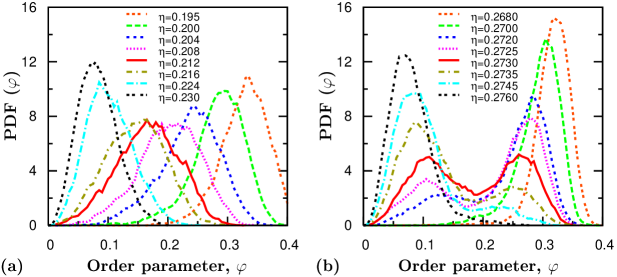
Figure 1: Probability distribution function (PDF) of the order parameter $\varphi$ for noise values $\eta$ around the critical point. A curve with one single peak indicates a second-order phase transition. Two peaks indicate a first-order phase transition. (a) Continuous, second-order phase transition for $v=0.1$. (Analogous behaviour can be observed at $v=0.03$.) (b) First-order phase transition at $v=0.5$. (The same behaviour can be observed for $v=1.0$ or $v=3.0$.) Other parameters: $\rho=1/8$, $L=64$, $N=32768$, $T=10^{6}$.

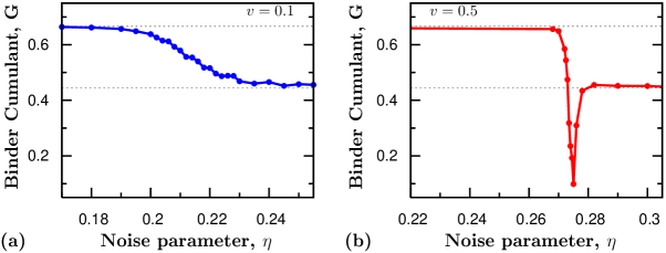
Figure 2: The Binder cumulant $G$ as a function of the noise $\eta$. The absence of a minimum point in $G$ (smooth behaviour) indicates a second-order phase transition, whereas its presence $G$ indicates a first-order phase transition. Values of $G$ in the ordered phase and in the disordered phase are denoted by horizontal lines at $G=2/3$ and $G=4/9$, respectively. (a) The behaviour of the Binder cumulant confirms that the phase transition at $v=0.1$ is of second-order. (The same behaviour can be observed for $v=0.03$.) (b) The definite minimum around $\eta=0.275$ means a first-order phase transition at $v=0.5$. (The same behaviour can be observed for $v=1.0$ or $v=3.0$) Other parameters: $\rho=1/8$, $L=64$, $N=32768$, $T=10^{6}$.

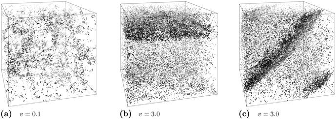
Figure 3: Snapshots of the spatial distribution of particles in the 3dSNM. The colour shading shows the distance of particles, particles in the far fade towards light gray. (a) A typical snapshot of the system in the small velocity regime ($v=0.1$). The isolated flocks moving coherently with a characteristic steady state size coexisting with a background gas of particles. (b) Particles move parallel to the edges of the simulation cube in the large velocity regime ($v=3.0$), and a density wave emerges. (c) Density wave moves diagonally ($v=3.0$). Other parameters: $\rho=1/8$, $L=64$, $N=32768$, $\eta=0.1$.

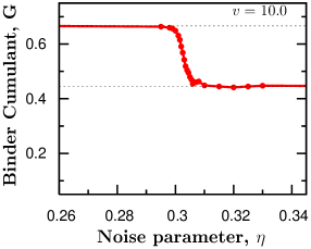
Figure 4: The Binder cumulant $G$ as a function of the noise at particle velocity $v=10.0$. $G$ has a smooth behaviour, indicating a second-order phase transition, but the value decreases significantly faster at the transition point. Values of $G$ in the ordered phase and in the disordered phase are denoted by horizontal lines at $G=2/3$ and $G=4/9$, respectively. Other parameters: $\rho=1/8$, $L=64$, $N=32768$, $T=10^{6}$.

3 Particle diffusion

In order to investigate the 3dSNM in more details and interpret the unusual change of the order of transition as a function of velocity, we have assessed the temporal divergence of neighbouring particles nagy . We locate pairs in the entire system, and in every simulation step we compute the average distance of the pairs

$$r(t)=\frac{1}{N_{p}}|\sum_{i=1}^{N_{p}}{d_{i}(t)}|,$$ (4)

where $r_{i}(t)$ is the distance between members of the $i$th pair at time $t$, and $N_{p}$ is the number of pairs with $r_{i}(t_{0})<R$ initially at time $t_{0}$. We evaluated both the parallel and the perpendicular components of the divergence, where parallel means a direction along the average velocity vector of all particles. To eliminate artifacts of the periodic boundary condition, we only use the data where $r(t)\leq\frac{1}{12}L$. Typical averaged square displacement curves as a function of time can be seen in (Fig. 5.).

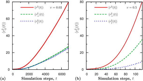
Figure 5: Averaged relative square displacements of neighbouring particles as a function of time. The perpendicular square displacement is the sum of two perpendicular directions. In order to compare this with the parallel (to $\langle v_{i}\rangle_{i})$) one, we divide the square displacement by two. (a) The diffusion is isotropic, $v=0.03$. At $v=0.1$ we can observe a little anisotropy in the diffusion, hence we name $v=0.1$ the border velocity between the large and small velocity regimes. (b) The diffusion is anisotropic; it is significantly larger in the perpendicular direction ($\langle r^{2}_{\bot}\rangle$) than in the parallel direction ($\langle r^{2}_{\|}\rangle$). On log-log scale we can observe the super-diffusion behaviour, as written in the text (graphs not shown). Other parameters: $\rho=1/8$, $L=64$, $N=32768$, $T=5*10^{5}$.

A super-diffusive gregoiretu1 behaviour occurs at medium diffusion times in the ordered state in both small and large velocity regimes, where $\alpha$ is greater than one ($\langle r^{2}\rangle(t)\sim t^{\alpha}$). At low noise levels three different mean square displacements can be observed. At short diffusion times particles keep their relative positions to each other; the diffusion is almost frozen ($\alpha\sim 0$). We assume that on this time scale most particles stay in the same locally ordered flock where they were when the pairs were formed. At intermediate times, when particles have time to change their flocks, a super-diffusive behaviour occurs. At this time scale, initially neighbouring particles diverge from each other linearly, due to the effects of the different flocks they belong to. In other words, the mean spatial separation of the particles increases approximately linearly or faster (e.g., turning away) with time (the flocks perform random walk only on a larger time scale), leading to a super-diffusive behaviour with an exponent of $\alpha\geq 2$. Finally, on large time scale the flocks themselves exhibit random walk movement and the distance of the pairs increases with an exponent $\alpha=1$.

In the large velocity regime we have also found an anisotropy in diffusion while in the small velocity regime the diffusion is isotropic. The diffusion in the perpendicular direction is greater than in the parallel one (shown in Fig. 5.). The ratio of the square displacement components $r^{2}_{\bot}/r^{2}_{\|}$ shows the level of anisotropy; it increases by the particle velocity. Because of the greater diffusion value in the perpendicular direction at large velocities density waves occur in three dimensions, similarly to the two dimensional, original SNM model nagy . The density waves in three dimensions are planes, the direction of the normal vector is parallel to the average velocity of all particles. It means that although we have found a definite minimum in the Binder cumulant, and the PDF graphs have two peaks, we can not exclude the possibility that these results are only an artificial outcome of the large velocity regime, caused by the periodic boundary conditions. The self-appending density waves may induce an artificial strengthening in the ordered state, causing the first-order phase transition-like behaviour ultimately.

4 Symmetry breaking in the directional distribution

The symmetry breaking in the diffusion in the large velocity regime is discussed in the previous section; it can cause the emergence of density waves. The density waves may have other signs too. If they occur, the directional distribution must have significant symmetry breaking, because moving in the direction parallel to the edges of the cube corresponds to a more stable state. With smaller possibility diagonal density waves also occur.

We have investigated the probability distribution function (PDF) of the direction of the averaged velocity of the particles, and we have found uniform distribution in the small velocity regime and anisotropic distribution at the large velocity regime (Fig. 6.). These results support our assumption that density waves do not occur at small particle velocities, until density waves emerge for larger particle velocities.

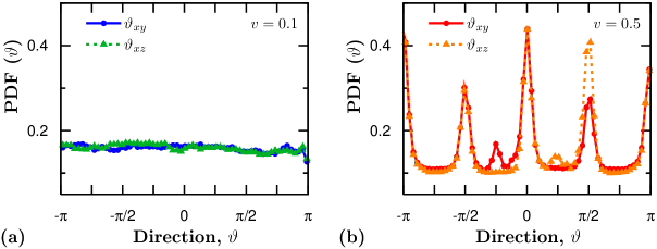
Figure 6: The directional distribution of the average velocity. $\vartheta_{xy}$, $\vartheta_{xz}$ denote the direction of the average velocity projected to plane $xy$, $xz$ respectively. (a) At low particle velocities the distribution is uniform ($v=0.1$). (b) At large particle velocities symmetry breaking occurs ($v=0.5$). The peaks at $\vartheta=k*\frac{\pi}{2}$ (where $k$ is integer) indicate that the particles movement is most likely along the edges of the cube. One can observe smaller peaks at $\vartheta=\frac{\pi}{4}$. Corresponding density waves move diagonally and have higher linear size, thus they less likely than the parallel ones. Other parameters: $\rho=1/8$, $L=64$, $N=32768$.

We emphasize that the original purpose of the Vicsek et. al. vicsek model is to interpret the collective movement of migrating cells, flocking birds or other biological systems, where the self-propelled particle velocity is small compared to the ratio of their interaction radius and reaction time $v\ll R/\tau$. With the parameters used this means that the velocity must be small compared to unity. Our investigation showed that velocity with the parameters used in three dimensions is $v\leq 0.1$.

5 Conclusions

We have found that the behaviour of the 3dSNM is similar to that of the SNM in two dimensions in many aspects. In the small velocity regime the order-disorder transition is of second-order, continuous phase transition just as in two-dimensions vicsek ; czirok . At this velocity values artificial symmetry breaking did not occur, thus the results have physical relevance to the biological systems.

In the large velocity regime a further discontinuous symmetry breaking occurs in the direction of the average velocity, not observed before for the 3d case. This indicates the emergence of density waves gregoire (showed earlier in two dimensions nagy ), caused by the anisotropic diffusion of initially neighbouring particles, due to the periodic boundary conditions. Hence we can not draw any conclusions about the physical behaviour of the 3dSNM in the large velocity regime. Finite size effects in the case of SPP models are very delicate, since they are due to the fact that in the ordered regime the particles run through the cell in a time linearly proportional to L, so they ”feel” the two opposite side of the system in a relatively short time interval. Going to larger sizes does not solve this problem, because, although the above ”scanning” time somewhat increases, the relative magnitude of the inherent fluctuations decreases and the effect of the rectangular symmetry of the simulational cell shows up even more markedly. This is a paradoxical situation needing further exploration. Finally, if the velocity and the linear size of the system are of the same order of magnitude, the system exhibits a continuous mean field like behaviour.

- (1) M. Nagy, I. Daruka, and T. Vicsek, Physica A 373, (2007) 445-454.
- (2) T. Vicsek, A. Czirók, E. Ben-Jacob, I. Cohen and O. Shochet Phys. Rev. Lett. 75, 1226 (1995).
- (3) A. Czirók, H. E. Stanley and T. Vicsek, J. Phys A 30, 1375 (1997).
- (4) Z. Csahók and T. Vicsek, Phys. Rev. E 52, 5297 (1995).
- (5) J. Toner and Y. Tu, Phys. Rev. Lett. 75, 4326 (1995).
- (6) J. Toner, Y. Tu and M. Ulm, Phys. Rev. Lett. 80, 4819 (1998).
- (7) J. Toner and Y. Tu, Phys. Rev. E 58, 4828 (1998).
- (8) A. Czirók, M. Vicsek and T. Vicsek, Physica A 264, (1999) 299-304.
- (9) G. Grégoire and H. Chaté, Phys. Rev. Lett. 92, 025702 (2004).
- (10) J. K. Parrish and W. M. Hammer Animal Groups in Three Dimensions, Cambridge University Press, Cambridge, 1997.
- (11) C. J. Feare, The starlings, Oxford University Press, 1984; J. K. Parrish and W. H. Hamner, eds., Animal groups in three dimensions, Cambridge University Press, 1997 (and references therein); C. W. Reynolds, Comp. Graph. 21, 25 (1987).
- (12) J. K. Parrish and L. Edelstein-Keshet, Science 284, 99 (1999); T. Inagaki, W. Sakamoto and T. Kuroki, Bull. Jap. Soc. Sci. Fish, 42, 265 (1976).
- (13) E. M. Rauch, M. M. Millonas and D. R. Chialvo, Phys. Lett. A, 207, 185 (1995).
- (14) E. Ben-Jacob, I. Cohen, O. Shochet, A. Czirók and T. Vicsek, Phys. Rev. Lett. 75, 2899 (1995); J. A. Shapiro, BioEssays 17, 597 (1995); J. A. Shapiro and M. Dworkin, eds., Bacteria as multicellular organisms, Oxford University Press, 1997.
- (15) K. Binder and D. W. Herrmann, Monte Carlo Simulation in Statistical Physics, Springer (1997).
- (16) C. Huepe and M. Aldana, Phys. Rev. Lett. 92, 168701 (2004).
- (17) M. Aldana, V. Dossetti, C. Huepe, V. M. Kenkre and H. Larralde Phys. Rev. Lett. 98, 095702 (2007)
- (18) G. Grégoire, H. Chaté and Y. Tu, Phys. Rev. E 64, 011902 (2001);