Frequency estimation based on the cumulated Lomb-Scargle periodogram

Abstract.

We consider the problem of estimating the period of an unknown periodic function observed in additive noise sampled at irregularly spaced time instants in a semiparametric setting. To solve this problem, we propose a novel estimator based on the cumulated Lomb-Scargle periodogram. We prove that this estimator is consistent, asymptotically Gaussian and we provide an explicit expression of the asymptotic variance. Some Monte-Carlo experiments are then presented to support our claims.

GET/Télécom Paris, CNRS LTCI

1. Introduction

The problem of estimating the frequency of a periodic function corrupted by additive noise is ubiquitous and has attracted a lot of research efforts in the last three decades. Up to now, most of these contributions have been devoted to regularly sampled observations; see e.g. Quinn and Hannan (2001) and the references therein. In many applications however, the observations are sampled at irregularly spaced time instants: examples occur in different fields, including among others biological rhythm research from free-living animals (Ruf (1999)), unevenly spaced gene expression time-series analysis (Glynn et al. (2006)), or the analysis of brightness of periodic stars (Hall et al. (2000); Thiebaut and Roques (2005)). In the latter case, for example, irregular observations come from missing observations due to poor weather conditions (a star can be observed on most nights but not all nights), and because of the variability of the observation times. In the sequel, we consider the following model:

$$Y_{j}=s_{\star}(X_{j})+\varepsilon_{j},\quad j=1,2,\dots,n\;,$$ (1)

where $s_{\star}$ is an unknown (real-valued) $T$–periodic function on the real line, $\{X_{k}\}$ are the sampling instants and $\{\varepsilon_{k}\}$ is an additive noise. Our goal is to construct a consistent, rate optimal and easily computable estimator of the frequency $f_{0}=1/T$ based on the observations $\{(X_{i},Y_{i})\}_{i=1,\dots,n}$ in a semiparametric setting, where $s_{\star}$ belongs to some function space. To our best knowledge, the only attempt to rigorously derive such semiparametric estimator is due to Hall, Reimann and Rice (2000), who propose to use the least-squares criterion defined by $S_{n}(f)=\sum_{k=1}^{n}\left(Y_{k}-\hat{s}(X_{k}|f)\right)^{2}$ where $\hat{s}(x|f)$ is a nonparametric kernel estimator of $s_{\star}(x)$, adapted to a given frequency $f$, from the observations $(X_{j},Y_{j}),\;j=1,\dots,n$. For an appropriate choice of $\hat{s}(x|f)$, the minimizer of $S_{n}(f)$ has been shown to converge at the parametric rate and to achieve the optimal asymptotic variance, see Hall et al. (2000).

Here, we propose to estimate the frequency by maximizing the Cumulated Lomb-Scargle Periodogram (CLSP), defined as

$$\Lambda_{n}(f)=\frac{1}{n^{2}}\sum_{k=1}^{K_{n}}\left|\sum_{j=1}^{n}Y_{j}\ \textrm{e}^{-2\textrm{i}k\pi fX_{j}}\right|^{2}\;,$$ (2)

where $K_{n}$ denotes the number of cumulated harmonics, assumed to be slowly increasing with $n$. Considering such an estimator is very natural since this procedure might be seen as an adaptation of the algorithm proposed by Quinn and Thomson (1991) obtained by replacing the periodogram by the Lomb-Scargle periodogram, introduced in Lomb (1976) (see also Scargle (1982)) to account for irregular sampling time instants. Note also that such an estimator can be easily implemented and efficiently computed using (Press et al., 1992, p. 581). We will show that the estimator based on the maximization of the cumulated Lomb-Scargle periodogram $\Lambda_{n}(f)$ is consistent, rate optimal and asymptotically Gaussian. It is known that frequency estimators based on the cumulated periodogram are optimal in terms of rate and asymptotic variance in the cases of continuous time observations and regular sampling (see Golubev (1988); Quinn and Thomson (1991); Gassiat and Lévy-Leduc (2006)). We will see that, somewhat surprisingly, at least under renewal assumptions on the observation times, the asymptotic variance is no longer optimal in the irregular sampling case investigated here. However, because of its numerical simplicity, we believe that the CLSP estimator is a sensible estimator, which may be used as a starting value of more sophisticated and computationally intensive techniques, see e.g.  Hall, Reimann and Rice (2000). The numerical experiments that we have conducted clearly support these findings.

The paper is organized as follows. In Section 2, we state our main results (consistency and asymptotic normality) and provides sketches of the proofs. In Section 3, we present some numerical experiments to compare the performances of our estimator with the estimator of Hall, Reimann and Rice (2000). In Section 4, we provide some auxiliary results and we detail the steps that are omitted in the proof sketches of the main results.

2. Main results

Define the Fourier coefficients of a locally integrable $T$-periodic function $s$ by

$$c_{k}(s)=\frac{1}{T}\int_{0}^{T}s(t)\,\textrm{e}^{-2\textrm{i}k\pi t/T}dt,\quad k\in\mathbb{Z}\quad\text{so that}\quad s(t)=\sum_{p\in\mathbb{Z}}c_{p}(s)\textrm{e}^{2\textrm{i}\pi pt/T}\;,$$ (3)

when this expansion is well defined. Recall that the frequency $f_{0}=1/T$ of $s_{\star}$ is here the parameter of interest. Consider the least-squares criterion based on observations $\{(X_{i},Y_{i})\}_{i=1,\dots,n}$,

$$L_{n}(f,\mathbf{c})=\sum_{j=1}^{n}\left(Y_{j}-\sum_{k=-K_{n}}^{K_{n}}c_{k}\ \textrm{e}^{2\textrm{i}k\pi fX_{j}}\right)^{2}\;,\quad{\mathbf{c}}=[c_{-K_{n}},\dots,c_{K_{n}}]^{T}$$ (4)

where $\{K_{n}\}$ is the number of harmonics. For a given frequency $f$, the coefficients $\tilde{\mathbf{c}}_{n}(f)=[\tilde{c}_{-K_{n}},\dots,\tilde{c}_{K_{n}}]$ which minimize (4) solve the system of equations $G_{n}(f)\tilde{\mathbf{c}}_{n}(f)=n\hat{\mathbf{c}}_{n}(f)$, where the (Gram) matrix $G_{n}(f)=[G_{n,k,l}(f)]_{-K_{n}\leq k,l\leq K_{n}}$ and the vector $\hat{\mathbf{c}}_{n}(f)=[\hat{c}_{-K_{n}}(f),\dots,\hat{c}_{K_{n}}(f)]$ are defined by:

$$G_{n,k,l}(f)=\sum_{j=1}^{n}\textrm{e}^{-2\textrm{i}(k-l)\pi fX_{j}}\quad\text{and}\quad\hat{c}_{l}(f)=\frac{1}{n}\sum_{j=1}^{n}Y_{j}\textrm{e}^{-2\textrm{i}l\pi fX_{j}}\;.$$ (5)

An estimator for the frequency $f_{0}$ can then be obtained by minimizing the residual sum of squares

$$f\mapsto L_{n}(f,\{\tilde{c}_{k}(f)\})=\sum_{j=1}^{n}Y_{j}^{2}-n^{2}\mathbf{\hat{c}}^{T}_{n}(f)G^{-1}_{n}(f)\mathbf{\hat{c}}_{n}(f)\;.$$ (6)

Note that computing $\tilde{\mathbf{c}}_{n}(f)$ is numerically cumbersome when $K_{n}$ is large since it requires to solve a system of $2K_{n}+1$ equations for each value of the frequency $f$ where the function $L_{n}(f,\{\tilde{c}_{k}(f)\})$ should be evaluated. In many cases (including the renewal case investigated below, see Lemmas 1 and 2), we can prove that, as $n$ goes to infinity, if the number of harmonics $K_{n}$ grows slowly enough (say, at a logarithmic rate), the Gram matrix $G_{n}(f)$ is approximately $G_{n}(f)\approx n\mathrm{Id}_{2K_{n}+1}$, where $\mathrm{Id}_{p}$ denotes the $p\times p$ identity matrix; this suggests to approximate $L_{n}(f,\{\tilde{c}_{k}(f)\})$ by $f\mapsto\sum_{j=1}^{n}Y_{j}^{2}-n\sum_{|k|\leq K_{n}}|\hat{c}_{k}(f)|^{2}$. The minimization of this quantity is equivalent to maximizing the cumulated periodogram $\Lambda_{n}$ defined by (2).

That is why we propose to estimate $f_{0}$ by $\hat{f}_{n}$ defined as follows,

$$\Lambda_{n}(\hat{f}_{n})=\sup_{f\in[f_{\min},f_{\max}]}\Lambda_{n}(f)\;,$$ (7)

where $[f_{\min},f_{\max}]$ is a given interval included in $(0,\infty)$. Consider the following assumptions.

1. $s_{\star}$ is a real-valued periodic function defined on $\mathbb{R}$ with finite fundamental frequency $f_{\star}$.

2. $\{X_{j}\}$ are the observation time instants, modeled as a renewal process, that is, $X_{j}=\sum_{k=1}^{j}V_{k}$, where $\{V_{k}\}$ is a an i.i.d sequence of non-negative random variables with finite mean. In addition, for all $\epsilon>0$, $\sup_{|t|\geq\epsilon}|\Phi(t)|<1$, where $\Phi$ denotes the characteristic function of $V_{1}$,

   $$\Phi(t)=\mathbb{E}[\exp(\textrm{i}tV_{1})]\;.$$ (8)

3. $\{\varepsilon_{j}\}$ are i.i.d. zero mean Gaussian random variables with (unknown) variance $\sigma_{\star}^{2}>0$ and are independent from the random variables $\{X_{j}\}$.

4. The distribution of $V_{1}$ has a non-zero absolutely continuous part with respect to the Lebesgue measure.

Recall that in (H1) the fundamental frequency is uniquely defined for non constant functions as follows: $T_{\star}=1/f_{\star}$ is the smallest $T>0$ such that $s_{\star}(t+T)=s_{\star}(t)$ for all $t$. All the possible frequencies of $s_{\star}$ are then $f_{\star}/l$, where $l$ is a positive integer. Note that the assumption made on the distribution of $V_{1}$ in (H2) is a Cramer’s type condition, which is weaker than (H4).

The following result shows that $\hat{f}_{n}$ is a consistent estimator of the frequency contained by $[f_{\min},f_{\max}]$ under very mild assumptions and give some preliminary rates of convergence. These rates will be improved in Theorem 2 under more restrictive assumptions.

Theorem 1.

Assume (H1)–(H3). Let $\{K_{n}\}$ be a sequence of positive integers tending to infinity such that

$$\lim_{n\to+\infty}K_{n}\left\{R(n^{\beta})+n^{-1/2+\beta}\right\}=0\quad\text{for some $\beta>0$}\;,$$ (9)

where

$$R(m)=\sum_{|k|>m}|c_{k}(s_{\star})|,\quad m\geq 0\;.$$ (10)

Let $\hat{f}_{n}$ be defined by (7) with $0<f_{\min}<f_{\max}$ such that $f_{0}$ is the unique number $f\in[f_{\min},f_{\max}]$ for which $s_{\star}$ is $1/f$–periodic. Then, for any $\alpha>0$,

$$\hat{f}_{n}=f_{0}+o_{p}(n^{-1+\alpha})\;.$$ (11)

If we assume in addition that $\mathbb{E}(V_{1}^{2})$ is finite, then

$$n(\hat{f}_{n}-f_{0})\to 0\quad a.s.$$ (12)

Proof (sketch).

Since $f_{\star}$ is the fundamental frequency of $s_{\star}$, the assumption on $[f_{\min},f_{\max}]$ is equivalent to saying that there exists a unique positive integer $\ell$ such that

$$f_{\min}\leq f_{\star}/\ell\leq f_{\max}\;,$$ (13)

and that $f_{\star}/\ell=f_{0}$. Using (1), we split $\Lambda_{n}$ defined in (2) into three terms: $\Lambda_{n}(f)=D_{n}(f)+\xi_{n}(f)+\zeta_{n}(f)$ where

$$D_{n}(f)=\frac{1}{n^{2}}\sum_{k=1}^{K_{n}}\left|\sum_{j=1}^{n}s_{\star}(X_{j})\ \textrm{e}^{-2\textrm{i}k\pi fX_{j}}\right|^{2}\;,$$ (14)

$$\xi_{n}(f)=\frac{2}{n^{2}}\sum_{k=1}^{K_{n}}\sum_{j,j^{\prime}=1}^{n}\cos\{2\pi kf(X_{j}-X_{j^{\prime}})\}\,s_{\star}(X_{j})\varepsilon_{j^{\prime}}\;,$$ (15)

$$\zeta_{n}(f)=\frac{1}{n^{2}}\sum_{k=1}^{K_{n}}\left|\sum_{j=1}^{n}\varepsilon_{j}\ \textrm{e}^{-2\textrm{i}k\pi fX_{j}}\right|^{2}\;.$$ (16)

We prove in Lemma 4 of Section 4 that $\xi_{n}+\zeta_{n}$ tends uniformly to zero in probability as $n$ tends to infinity. Then, by Lemmas 5 and 6 proved in Section 4.2, for any $\alpha$, $D_{n}$ is maximal in balls centered at sub-multiples of $f_{\star}$ with radii of order $n^{-1+\alpha}$ with probability tending to 1. Since, by (13), the interval $[f_{\min},f_{\max}]$ contains but the sub-multiple $f_{\star}/\ell=f_{0}$, $\hat{f}_{n}$ satisfies (11). This line of reasoning is detailed in Section 4.3. The obtained rate is then refined in (12) by adapting the consistency proof of Quinn and Thomson (1991) to our random design context (see Section 4.4). ∎

Remark 1.

One can construct a sequence $\{K_{n}\}$ satisfying Condition (9), as soon as

$$\sum_{k\in\mathbb{Z}}|c_{k}(s_{\star})|<+\infty\;,$$ (17)

which is a very mild assumption.

Remark 2.

Observe that $f_{0}=f_{\star}$ in Theorem 1 if and only if $f_{\star}/2<f_{\min}\leq f_{\star}\leq f_{\max}$.

Remark 3.

If $f_{\min}$ and $f_{\max}$ are such that $s_{\star}$ has several frequencies in $[f_{\min},f_{\max}]$, that is, (13) has multiple solutions $\ell=l_{\min},\dots,l_{\max}$, by partitioning $[f_{\min},f_{\max}]$ conveniently, we get instead of (11) (resp. (12)) that there exists a random sequence $(\ell_{n})$ with values in $\{l_{\min},\dots,l_{\max}\}$ such that $\hat{f}_{n}=f_{\star}/\ell_{n}+o_{p}(n^{-1+\alpha})$ (resp. $n(\hat{f}_{n}-f_{\star}/\ell_{n})\to 0$). This is not specific to our estimator. Unless an appropriate procedure is used to select the largest plausible frequency, any standard frequency estimators will in fact converge to a set of sub-multiples of $f_{\star}$.

We now derive a Central Limit Theorem which holds for our estimator when Condition (9) is strengthened into (18) and (19) and a finite fourth moment is assumed on $V_{1}$.

Theorem 2.

Assume (H1)–(H4). Assume in addition that $\mathbb{E}[V_{1}^{4}]$ is finite and that $s_{\star}$ satisfies

$$\sum_{k\in\mathbb{Z}}|k|^{3}|c_{k}(s_{\star})|<+\infty\;.$$ (18)

Let $\{K_{n}\}$ be a sequence of positive integers tending to infinity such that

$$\lim_{n\to+\infty}K_{n}n^{-\epsilon}=0\quad\text{for all}\quad\epsilon>0\;.$$ (19)

Let $\hat{f}_{n}$ be defined by (7) with $0<f_{\min}<f_{\max}$ such that $f_{0}$ is the unique number $f\in[f_{\min},f_{\max}]$ for which $s_{\star}$ is $1/f$–periodic. Then we have the following asymptotic linearization:

$$n^{3/2}(\hat{f}_{n}-f_{0})=\frac{\mu\;f_{0}}{n^{3/2}\sigma_{\star}^{2}f_{\star}^{2}I_{\star}}\sum_{j=1}^{n}\left(j-\frac{n}{2}\right)\dot{s}_{\star}(X_{j})\left(\varepsilon_{j}+s_{\star}(X_{j})\right)+o_{p}(1)\;,$$ (20)

where $\mu=\mathbb{E}(V_{1})$ and

$$I_{\star}=\frac{\mu^{2}}{12\sigma_{\star}^{2}f_{\star}}\int_{0}^{1/f_{\star}}\dot{s}_{\star}^{2}(t)dt\;.$$ (21)

Moreover $\hat{f}_{n}$ satisfies the following Central Limit Theorem

$$n^{3/2}(\hat{f}_{n}-f_{0})\frac{f_{\star}}{f_{0}}\stackrel{{\scriptstyle\mathcal{L}}}{{\longrightarrow}}\mathcal{N}(0,\check{\sigma}^{2}),$$ (22)

where

$$\check{\sigma}^{2}=I_{\star}^{-1}\left\{1+\frac{\displaystyle\sum_{k\neq 0}|c_{k}(s_{\star}\dot{s}_{\star})|^{2}\left(\frac{1-|\Phi(2k\pi f_{\star})|^{2}}{|1-\Phi(2k\pi f_{\star})|^{2}}\right)}{\sigma_{\star}^{2}\sum_{k\in\mathbb{Z}}|c_{k}(\dot{s}_{\star})|^{2}}\right\},$$ (23)

where $\Phi$, defined in (8), denotes the characteristic function of $V_{1}$ and $\{c_{k}(s),k\in\mathbb{Z}\}$ denote the Fourier coefficients of a $1/f_{\star}$-periodic function $s$ as defined in (3) with $T=1/f_{\star}$.

Proof (sketch).

To derive (20), we use a Taylor expansion of $\dot{\Lambda}_{n}(f)$, the first derivative of $\Lambda_{n}(f)$ with respect to $f$, which provides

$$\dot{\Lambda}_{n}(\hat{f}_{n})=\dot{\Lambda}_{n}(f_{0})+(\hat{f}_{n}-f_{0})\ddot{\Lambda}_{n}(f^{\prime}_{n}),$$

where $f^{\prime}_{n}$ is random and lies between $\hat{f}_{n}$ and $f_{0}$. We prove in Sections 4.5 and 4.6 that

$$\dot{\Lambda}_{n}(f_{0})=\sum_{j=1}^{n}\left(\frac{X_{j}}{n}-\frac{\mu}{2}\right)\frac{\dot{s}_{\star}(X_{j})}{f_{0}}\left(\varepsilon_{j}+s_{\star}(X_{j})\right)+o_{p}(\sqrt{n}),$$ (24)

$$\ddot{\Lambda}_{n}(f^{\prime}_{n})=-n^{2}\frac{\mu^{2}}{12\;f_{0}}\int_{0}^{1/f_{0}}\dot{s}_{\star}^{2}(t)dt+o_{p}(n^{2}).$$ (25)

Since $\dot{s}_{\star}^{2}$ is $1/f_{\star}$-periodic and $f_{\star}/f_{0}$ is an integer, we have

$$\frac{\mu^{2}}{12}\int_{0}^{1/f_{0}}\dot{s}_{\star}^{2}(t)dt=\frac{\mu^{2}f_{\star}}{12\;f_{0}}\int_{0}^{1/f_{\star}}\dot{s}_{\star}^{2}(t)dt=\frac{\sigma_{\star}^{2}f_{\star}^{2}I_{\star}}{f_{0}}$$

The last three displayed equations and the assumption on $\dot{\Lambda}_{n}(\hat{f}_{n})$ thus yield

$$n^{3/2}(\hat{f}_{n}-f_{0})=\frac{f_{0}}{\sigma_{\star}^{2}f_{\star}^{2}I_{\star}\;n^{3/2}}\sum_{j=1}^{n}\left(X_{j}-\frac{n\mu}{2}\right)\dot{s}_{\star}(X_{j})\left(\varepsilon_{j}+s_{\star}(X_{j})\right)(1+o_{p}(1))+o_{p}(1)\;,$$

and Relations (20) and (22) then follow from

$$n^{-3/2}\sum_{j=1}^{n}\left(X_{j}-j\mu\right)\dot{s}_{\star}(X_{j})\varepsilon_{j}=o_{p}(1)\ \text{and}\ n^{-3/2}\sum_{j=1}^{n}\left(X_{j}-j\mu\right)\dot{s}_{\star}(X_{j})s_{\star}(X_{j})=o_{p}(1)\;,$$ (26)

$$S_{n}=\frac{\mu}{n^{3/2}\sigma_{\star}^{2}f_{\star}I_{\star}}\sum_{j=1}^{n}\left(j-n/2\right)\dot{s}_{\star}(X_{j})\left(\varepsilon_{j}+s_{\star}(X_{j})\right)\stackrel{{\scriptstyle\mathcal{L}}}{{\longrightarrow}}\mathcal{N}(0,\check{\sigma}^{2})\;.$$ (27)

The proof of (26) follows from straightforward computations and is not detailed here. We conclude with the proof of (27). By (H3), we have $S_{n}\stackrel{{\scriptstyle d}}{{=}}\frac{\mu}{\sigma_{\star}^{2}f_{\star}I_{\star}}\left(A_{n}Z+U_{n}\right)$ where $A_{n}=n^{-3/2}\left(\sum_{j=1}^{n}\left(j-\frac{n}{2}\right)^{2}{\dot{s}_{\star}}^{2}(X_{j})\right)^{1/2}$, $U_{n}={n^{-3/2}}\sum_{j=1}^{n}\left(j-n/2\right)(s_{\star}\dot{s}_{\star})(X_{j})$ and $Z$ has distribution $\mathcal{N}(0,\sigma_{\star}^{2})$ and is independent from the $X_{j}$’s. Therefore, since $Z$ and $U_{n}$ are independent, (27) follows from the two assertions

$$A_{n}=\left(\frac{1}{12}c_{0}({\dot{s}_{\star}}^{2})\right)^{1/2}(1+o_{p}(1))\;;$$ (28)

$$\frac{\mu}{\sigma_{\star}^{2}f_{\star}I_{\star}}U_{n}\stackrel{{\scriptstyle\mathcal{L}}}{{\longrightarrow}}\mathcal{N}\left(0,\frac{\sum_{k\neq 0}|c_{k}(s_{\star}\dot{s}_{\star})|^{2}\left(\frac{1-|\Phi(2k\pi f_{\star})|^{2}}{|1-\Phi(2k\pi f_{\star})|^{2}}\right)}{I_{\star}\,\sigma_{\star}^{2}\sum_{k\in\mathbb{Z}}|c_{k}(\dot{s}_{\star})|^{2}}\right)\;.$$ (29)

Assertions (28) and (29) follow straightforwardly from (53) and (54) in Proposition 1 respectively. ∎

Remark 4.

If the $\{V_{k}\}$ are exponentially distributed (the sampling scheme is a Poisson process), then (23) yields $\check{\sigma}^{2}=I_{\star}^{-1}\left\{1+\|s_{\star}\dot{s}_{\star}\|_{2}^{2}/(\sigma_{\star}^{2}\|\dot{s}_{\star}\|_{2}^{2})\right\},$ $\|\cdot\|_{p}$ denoting the usual $L^{p}$ norm on $[0,1/f_{\star}]$.

In Gassiat and Lévy-Leduc (2006), the local asymptotic normality (LAN) of the semiparametric model (1) is established for regular sampling with decreasing sampling instants. Their arguments can be extended to the irregular sampling scheme. More precisely, any estimator satisfying the asymptotic linearization

$$n^{3/2}(\bar{f}_{n}-f_{\star})=\left(\frac{\mu}{n^{3/2}\sigma_{\star}^{2}f_{\star}I_{\star}}\sum_{j=1}^{n}\left(j-\frac{n}{2}\right)\dot{s}_{\star}(X_{j})\varepsilon_{j}\right)(1+o_{p}(1))\;,$$ (30)

where $I_{\star}$ is defined in (21), is an efficient semiparametric estimator of $f_{\star}$ in the sense of McNeney and Wellner (2000). As a byproduct of the proof of Theorem 2, one has that the right hand-side of (30) is asymptotically normal with mean zero and variance $I_{\star}^{-1}$. Hence $I_{\star}^{-1}$ is the optimal asymptotic variance. In view of (20) and (22), we see that the linearization of our estimator $\hat{f}_{n}$ contains an extra term since $\varepsilon_{j}$ in (30) is replaced by $(\varepsilon_{j}+s_{\star}(X_{j}))$ in (20). This extra term leads to an additional term in the asymptotic variance (23), which highly depends on the distribution of the $V_{k}$’s. Hence our estimator enjoys the optimal $n^{-3/2}$ rate but is not efficient. The estimator proposed in Hall et al. (2000) is efficient and thus, in theory, outperforms the CLSP estimator. On the other hand, our estimator is numerically more tractable, and it does not require a preliminary consistent estimator. In contrast, an interval containing the true frequency with size at $o_{p}(n^{-(3/2-1/12)})$ is required in the assumptions of Hall et al. (2000) (see p.554 after conditions (a)–(e)) and, whether this assumption is necessary is an open question. Nevertheless, since our estimator is rate optimal, it can be used as a preliminary estimator to the one of Hall, Reimann and Rice (2000).

3. Numerical experiments

Let us now apply the proposed estimator to periodic variable stars which are known to emit light whose intensity, or brightness, changes over time in a smooth and periodic manner. The estimation of the period is of direct scientific interest, for instance as an aid to classifying stars into different categories for making inferences about stellar evolution. The irregularity in the observation is often due to poor weather conditions and to instrumental constraints.

We benchmark the CLSP estimator with the least-squares method (see (6)), which is reported as giving the best empirical results in an extended simulation experiment which can be found in Hall et al. (2000). In this Monte-Carlo experiment, we generate synthetic observations corresponding to model (1) where the underlying deterministic function $s_{\star}$ is obtained by fitting a trigonometric polynomial of degree 6 to the observations of a Cepheid variable star avalaible from the MACHO database (http://www.stat.berkeley.edu/users/rice/UBCWorkshop). Figure 1 displays in its left part the observations of the Cepheid as points with coordinates $(X_{j}~{}\textrm{modulo}~{}3.9861,Y_{j})$, where $3.9861$ is the known period of the Cepheid and the $X_{j}$ are the observation times given by the MACHO database. In the right part of Figure 1, the observations $(X_{j},s_{\star}(X_{j}))$ are displayed as points with coordinates $(X_{j}~{}\textrm{modulo}~{}3.9861,s_{\star}(X_{j}))$ where $s_{\star}$ is a trigonometric polynomial of degree 6 fitted to the observations of the Cepheid variable star that we shall use.

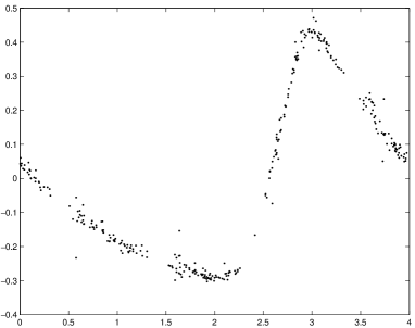
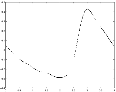
Figure 1. Left: Cepheid observations, Right: Trigonometric polynomial $s_{\star}$ fitted to the Cepheid observations.

Let us now describe further the framework of our experiments. The inter-arrivals $\{V_{k}\}$ have an exponential distribution with mean $1/5$. The additive noise is i.i.d. Gaussian with standard deviations equal to 0.07 and 0.23 respectively (the corresponding signal to noise ratios (SNR) are 10dB and 0dB). Typical realizations of the observations that we process are shown in Figure 2 when $f_{\star}=0.25$ and $n=300$ in the two previous cases on the left and right side respectively. More precisely, the observations $(X_{j},Y_{j})$ are displayed as stars with coordinates $(X_{j}~{}\textrm{modulo}~{}1/f_{\star},Y_{j})$ and the observations $(X_{j},s_{\star}(X_{j}))$ of the underlying function $s_{\star}$ are displayed as points with coordinates: $(X_{j}~{}\textrm{modulo}~{}1/f_{\star},s_{\star}(X_{j}))$. Since $E(V_{1})=1/5$, $n=300$ and $1/f_{\star}=4$ approximately 15 periods are overlaid.

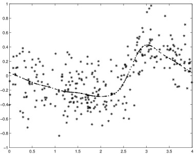
Figure 2. Deterministic signal (’.’) and noisy observations (’$\ast$’) with SNR=10dB (left) and 0dB (right).

The least-squares and cumulated periodogram criteria ($L_{n}$ and $\Lambda_{n}$) are maximized on a grid ranging from 0.2 to 0.52 with regular mesh $5\times 10^{-5}$. Since the fundamental frequency is equal to 0.25, the chosen range does not contain a sub-multiple of the fudamental frequency but a multiple. Hence we are in the case $\ell=1$ in (13), see Remark 3. We used $K_{n}=1,2,4,6,8$. The results of 100 Monte-Carlo experiments are summarized in Table 1. We display the biases, the standard deviations (SD) and the optimal standard deviations forecast by the theoretical study when $n=300,600$ and SNR=10dB, 0dB.

	SNR=10dB				SNR=0dB
	$n=300$		$n=600$		$n=300$		$n=600$
Optimal SD	$1.21\times 10^{-4}$		$4.28\times 10^{-5}$		$3.83\times 10^{-4}$		$1.35\times 10^{-4}$
Method	Bias$\times 10^{-5}$	SD $\times 10^{-4}$	Bias $\times 10^{-5}$	SD$\times 10^{-4}$	Bias$\times 10^{-4}$	SD $\times 10^{-4}$	Bias $\times 10^{-5}$	SD$\times 10^{-4}$
LS1	2.30	3.03	0.20	1.25	1.00	6.81	5.80	2.62
CP1	7.70	5.13	3.28	2.11	0.00	8.20	7.20	2.91
LS2	4.50	1.73	0.24	0.66	1.12	4.84	3.60	1.85
CP2	5.90	4.09	-0.16	1.76	0.49	6.88	2.50	2.12
LS4	1.99	1.15	0.00	0.48	0.79	4.67	3.70	1.45
CP4	1.89	3.83	-3.08	1.58	0.31	6.07	1.99	2.13
LS6	1.30	1.13	-0.40	0.48	0.97	5.38	2.40	1.44
CP6	-2.20	4.23	-2.96	1.75	0.37	7.58	2.70	2.22
LS8	0.60	1.19	-0.24	0.50	1.24	6.33	2.10	1.63
CP8	-1.30	5.28	-2.32	1.75	0.79	9.02	4.40	2.72

Table 1. Biases, standard deviations of the frequency estimates for different methods: Least-squares (LS1, LS2, LS4, LS6, LS8), Cumulated Periodogram (CP1, CP2, CP4, CP6, CP8) with $K_{n}=1,2,4,6,8$.

From the results gathered in Table 1, we get that the least-squares estimator produces better results than the CLSP estimator. Nevertheless, the CLSP estimator can be used as an accurate preliminary estimator of the frequency since its computational cost is lower than the one of the least-squares estimator. For both estimators, the parameter $K_{n}$ has to be chosen carefully in order to achieve the best trade-off between bias and variance. Finding a way of choosing $K_{n}$ adaptively is left for future research.

4. Detailed proofs

In this section we provide some important intermediary results and we detail the arguments sketched in the proofs of Section 2.

4.1. Technical lemmas

The following Lemma provides upper bounds for the moments of the empirical characteristic function of $X_{1},\dots,X_{n}$,

$$\varphi_{n,X}(t)=\frac{1}{n}\sum_{j=1}^{n}\textrm{e}^{\textrm{i}tX_{j}}\;.$$ (31)

Lemma 1.

Let (H2) hold. Then, for any non-negative integer $k$, there exists a positive constant $C$ such that for all $t\in\mathbb{R}$,

$$\left|\mathbb{E}[\varphi_{n,X}^{(k)}(t)]\right|\leq C\,\max_{1\leq l\leq k}\mathbb{E}[V_{1}^{l}]\,n^{k-1}(n\wedge|t|^{-1})\leq C\,(1+\mathbb{E}(V_{1}^{k}))\,n^{k-1}(n\wedge|t|^{-1})\;,$$ (32)

$$\mathbb{E}\left[\left|\varphi_{n,X}^{(k)}(t)\right|^{2}\right]\leq\mathbb{E}(V_{1}^{2k})n^{2k-1}+C(1+\mathbb{E}(V_{1}^{k}))n^{2k-1}(n\wedge|t|^{-1})\;.$$ (33)

The proof of Lemma 1 is omitted since it comes from straightforward algebra. The following Lemma provides an exponential deviation inequality for $\varphi_{n,X}$ defined in (31).

Lemma 2.

Under Assumption (H2), we have, for all $x>0$ and $t\in\mathbb{R}$,

$$\mathbb{P}\left(\left|\varphi_{n,X}(t)-\mathbb{E}(\varphi_{n,X}(t))\right|\geq x\right)\leq 4\exp\left(-\frac{nx^{2}\left|1-\Phi(t)\right|}{16(2+\sqrt{2})}\right),$$ (34)

where $\Phi$ is the characteristic function of $V$ defined in (8).

Proof.

Note that $\prod_{k=1}^{j}\textrm{e}^{\textrm{i}tV_{k}}-\Phi^{j}(t)=\sum_{q=1}^{j}\Phi^{j-q}(t)\Pi_{q}(t)$ where $\Pi_{q}(t)=\prod_{k=1}^{q}\textrm{e}^{\textrm{i}tV_{k}}-\Phi(t)\prod_{k=1}^{q-1}\textrm{e}^{\textrm{i}tV_{k}}\;.$ Thus,

$$n\left(\varphi_{n,X}(t)-\mathbb{E}\left[\varphi_{n,X}(t)\right]\right)=\sum_{j=1}^{n}\left[\left(\prod_{k=1}^{j}\textrm{e}^{\textrm{i}tV_{k}}\right)-\Phi^{j}(t)\right]=\sum_{j=1}^{n}\sum_{q=1}^{j}\Phi^{j-q}(t)\Pi_{q}(t)=\sum_{q=1}^{n}\alpha_{n,q}(t)\Pi_{q}(t)$$

where $\alpha_{n,q}(t)=\sum_{j=q}^{n}\Phi^{j-q}(t)=(1-\Phi(t))^{-1}(1-\Phi^{n-q+1}(t)),$ the last equality being valid as soon as $\Phi(t)\neq 1$. Let $\mathcal{F}_{q}$ denotes the $\sigma$-field generated by $V_{1},\dots,V_{q}$. Note that $\left\{\alpha_{n,q}(t)\Pi_{q}(t),\ q\geq 1\right\}$ is a martingale difference adapted to the filtration $(\mathcal{F}_{q})_{q\geq 1}$ and

$$|\alpha_{n,q}(t)\Pi_{q}(t)|\leq 4|1-\Phi(t)|^{-1}\quad\text{and}\quad\mathbb{E}^{\mathcal{F}_{q-1}}\left[|\alpha_{n,q}(t)\Pi_{q}(t)|^{2}\right]\leq\frac{4(1-|\Phi(t)|^{2})}{|1-\Phi(t)|^{2}}\leq 8|1-\Phi(t)|^{-1}\;,$$

where $\mathbb{E}^{\mathcal{F}_{q}}$ denotes the conditional expectation given $\mathcal{F}_{q}$. The proof then follows from Bernstein inequality for martingales (see Steiger (1969) or Freedman (1975)). ∎

For completeness, we state the following result, due to Golubev (1988).

Lemma 3.

Let $\mathcal{L}$ be a stochastic process defined on an interval $I\subseteq\mathbb{R}$. Then, for all $\lambda,R>0$,

$$\mathbb{P}\left(\sup_{\tau\in I}\mathcal{L}(\tau)>R\right)\leq\textrm{e}^{-\lambda R}\sup_{\tau\in I}\left(\sqrt{\mathbb{E}\left(\textrm{e}^{2\lambda\mathcal{L}(\tau)}\right)}\right)\left(1+\lambda\int_{\tau\in I}\sqrt{\mathbb{E}\left(\left|\dot{\mathcal{L}}(\tau)\right|^{2}\right)}d\tau\right).$$

4.2. Useful intermediary results

We present here some intermediary results which may be of independent interest.

Lemma 4.

Assume (H2)-(H3) and that $s_{\star}$ is bounded. Define $\xi_{n}(f)$ and $\zeta_{n}(f)$ by (15) and (16) where $(K_{n})$ is a sequence tending to infinity at most with a polynomial rate. Then, for any $0<f_{\min}<f_{\max}$, $\delta>0$ and $q=0,1,\dots$,

$$\sup_{f\in[f_{\min},f_{\max}]}\left|\xi^{(q)}_{n}(f)+\zeta^{(q)}_{n}(f)\right|=o_{p}(K_{n}^{q+1}n^{q-1/2+\delta})\;,$$ (35)

where, for any function $h$, $h^{(q)}$ denotes the $q$-th derivative of $h$.

Proof.

By (15) and (16),

$$\xi^{(q)}_{n}(f)=2\frac{(2\pi)^{q}}{n^{2}}\sum_{k=1}^{K_{n}}k^{q}L_{q}(X,kf)^{T}\varepsilon\;,\quad\zeta^{(q)}_{n}(f)=\frac{(2\pi)^{q}}{n^{2}}\sum_{k=1}^{K_{n}}k^{q}\varepsilon^{T}\Gamma_{q}(X,kf)\varepsilon\;,$$ (36)

where $\varepsilon=[\varepsilon_{1},\dots,\varepsilon_{n}]^{T}$, $L_{q}(X,f)=\left[\sum_{j=1}^{n}(X_{j}-X_{j^{\prime}})^{q}\cos^{(q)}\left\{2\pi f(X_{j}-X_{j^{\prime}})\right\}s_{\star}(X_{j})\right]_{1\leq j^{\prime}\leq n}$ and $\Gamma_{q}(X,f)=\left[\textrm{i}^{q}(X_{l}-X_{j})^{q}\textrm{e}^{2\textrm{i}\pi(X_{l}-X_{j})f}\right]_{1\leq l,j\leq n}$. Hence,

$$\sup_{f\in[f_{\min},f_{\max}]}\left|\xi^{(q)}_{n}(f)+\zeta^{(q)}_{n}(f)\right|\leq C\,n^{-2}\,K_{n}^{q+1}\sup_{0<f\leq K_{n}f_{\max}}\left|2L^{T}_{q}(X,f)\varepsilon+\varepsilon^{T}\Gamma_{q}(X,f)\varepsilon\right|\;.$$ (37)

Note that $\textrm{Tr}[\Gamma_{q}(X,f)]=0$ for $q\geq 1$, $\textrm{Tr}[\Gamma_{q}(X,f)]=n$ for $q=0$ and that the spectral radius of the matrix $\Gamma_{q}(X,f)$ is at most $\sup_{j=1,\dots,n}\sum_{l=1}^{n}|X_{l}-X_{j}|^{q}\leq nX_{n}^{q}$. For any hermitian matrix $\Lambda$ having all its eigenvalues less than $1/4$, $\mathbb{E}\left[\exp(Z^{T}\Lambda Z)\right]\leq\exp(\textrm{Tr}(\Lambda)+2\textrm{Tr}(\Lambda^{2}))$. Therefore, for any $\lambda>0$, on the event $\left\{\lambda\sigma^{\star\,2}nX_{n}^{q}\leq 1/8\right\}$,

$$\mathbb{E}\left[\left.\textrm{e}^{\lambda(2L_{q}(X,f)^{T}\varepsilon+\varepsilon^{T}\Gamma_{q}(X,f)\varepsilon)}\right|X\right]\leq C^{\prime}\exp\left\{C\lambda^{2}\left(L_{q}(X,f)^{T}L_{q}(X,f)+\textrm{Tr}(\Gamma_{q}^{2}(X,f))\right)\right\}\\ \leq C^{\prime}\exp\left\{C\lambda^{2}n^{3}X_{n}^{2q}\right\}\;,$$

where we have used $L^{T}_{q}(X,f)L_{q}(X,f)\leq Cn^{3}X_{n}^{2q}$ and $\textrm{Tr}[\Gamma_{q}^{2}(X,f)]\leq Cn^{2}X_{n}^{2q}$. Using (H3), we similarly get that $\mathbb{E}\left[\left.|L_{q}(X,f)^{T}\varepsilon|^{2}\right|X\right]\leq CL_{q}^{T}(X,f)L_{q}(X,f)\leq Cn^{3}X_{n}^{2q}$ and

$$\mathbb{E}\left[\left.|\varepsilon^{T}\Gamma_{q}(X,f)\varepsilon|^{2}\right|X\right]\leq C\textrm{Tr}[\Gamma^{2}_{q}(X,f)]\leq C\,n^{2}X_{n}^{2q}\;.$$ (38)

Applying Lemma 3, we get that, for all positive numbers $\lambda$ and $R$, on the event $\{\lambda\sigma^{\star\,2}nX_{n}^{q}\leq 1/8\}$,

$$\mathbb{P}\left[\left.\sup_{0<f\leq K_{n}f_{\max}}\left|2L_{q}(X,f)^{T}\varepsilon+\varepsilon^{T}\Gamma_{q}(X,f)\varepsilon\right|\geq R\right|X\right]\leq\\ C^{\prime}\,\textrm{e}^{-\lambda R+C\lambda^{2}n^{3}X_{n}^{2q}}\,\left(1+C\,K_{n}\,\lambda\,n^{3/2}\,X_{n}^{q+1}\right)\;.$$

Let $\delta>0$. Applying this inequality with $\lambda=n^{-3/2}X_{n}^{-q}$ and $R=n^{\delta+3/2}X_{n}^{q}$, we get

$$\mathbb{P}\left[\left.\sup_{0<f\leq K_{n}f_{\max}}\left|2L_{q}(X,f)^{T}\varepsilon+\varepsilon^{T}\Gamma_{q}(X,f)\varepsilon\right|\geq n^{\delta+3/2}X_{n}^{q}\right|X\right]\leq C\,\exp(-n^{\delta})\,\left(1+K_{n}\,X_{n}\right)\;.$$

Now, using (37), $\mathbb{P}\left(\sup_{f\in[f_{\min},f_{\max}]}\left|\xi_{n}^{(q)}(f)+\zeta_{n}^{(q)}(f)\right|\geq n^{q-1/2+2\delta}K_{n}^{q+1}\right)$

$$\leq \mathbb{P}\left(\sup_{0<f\leq K_{n}f_{\max}}\left|2L_{X}(f)^{T}\varepsilon+\varepsilon^{T}\Gamma_{X}(f)\varepsilon\right|\geq n^{\delta+3/2}X_{n}^{q}\right)+\mathbb{P}\left(X_{n}^{q}\geq n^{q+\delta}\right)$$

$$\leq C\,\exp(-n^{\delta})\,\left(1+K_{n}\,n\right)+n^{-\delta/q}\;,$$

which concludes the proof. ∎

Let us introduce the following notation. For some sequence $(\gamma_{n})$, and $f_{\star}>0$, we define, for any positive integers $n,j$ and $l$,

$$B_{n}(j,l)=[f_{\min},f_{\max}]\cap\{f~{}:~{}|f-jf_{\star}/l|\leq\gamma_{n}\}\textrm{ and }B_{n}^{c}(j,l)=[f_{\min},f_{\max}]\setminus B_{n}(j,l)\;.$$ (39)

Lemma 5.

Assume (H1)–(H2) and that $s_{\star}$ satisfies (17). Define $D_{n}(f)$ by (14), with a sequence $(K_{n})$ tending to infinity. Then, for any $\epsilon>0$, as $n$ tends to infinity,

$$\sup_{f\in\bigcap_{j,l}B_{n}^{c}(j,l)}D_{n}(f)=O_{p}\left(K_{n}R(m_{n})^{2}+\frac{\{K_{n}\,n\,m_{n}\}^{\epsilon}}{n\gamma_{n}}\right)\;,$$

where $(m_{n})$ is a sequence of positive integers, $R$ is defined by (10), $\bigcap_{j,l}$ is the intersection over integers $j\geq 1$, $l=1,\dots,K_{n}$ and $B_{n}^{c}(j,l)$ is defined by (39) with $0<f_{\min}<f_{\max}$ and $(\gamma_{n})$ satisfying

$$K_{n}\gamma_{n}\to 0\quad\text{and}\quad n\gamma_{n}\to\infty\;.$$ (40)

Proof.

We use the Fourier expansion (3) of $s_{\star}$ defined with the minimal period $T=1/f_{\star}$. Expanding $s_{\star}$ in (14) and using the definition of $\varphi_{n,X}$ in (31) and of $R(m)$ in (10), we get

$$D_{n}(f) \leq 2\sum_{k=1}^{K_{n}}\left|\sum_{|p|\leq m}c_{p}(s_{\star})\varphi_{n,X}\left\{2\pi(pf_{\star}-kf)\right\}\right|^{2}+2K_{n}R(m)^{2}$$ (41)

$$\leq 4\sum_{k=1}^{K_{n}}\left|\sum_{|p|\leq m}c_{p}(s_{\star})\mathbb{E}\left[\varphi_{n,X}\left\{2\pi(pf_{\star}-kf)\right\}\right]\right|^{2}+4\tilde{D}_{n,m}(f)+2K_{n}R(m)^{2}\;,$$

where we defined

$$\tilde{D}_{n,m}(f)=\sum_{k=1}^{K_{n}}\left|\sum_{|p|\leq m}c_{p}(s_{\star})\left(\varphi_{n,X}\left\{2\pi(pf_{\star}-kf)\right\}-\mathbb{E}\left[\varphi_{n,X}\left\{2\pi(pf_{\star}-kf)\right\}\right]\right)\right|^{2}\;.$$ (42)

For all positive integers $j$ and $l\leq K_{n}$, and $f\in\mathsf{A}_{n}=\bigcap_{j^{\prime},l^{\prime}}B_{n}^{c}(j^{\prime},l^{\prime})$, $2\pi|jf_{\star}-lf|\geq 2\pi l\gamma_{n}$. Thus, using (32) with $k=0$ in Lemma 1, (17), and $\lim_{n\to\infty}n\gamma_{n}=\infty$, we get, for all $f\in\mathsf{A}_{n}$, and $n$ large enough,

$$\sum_{k=1}^{K_{n}}\left|\sum_{|p|\leq m}c_{p}(s_{\star})\mathbb{E}\left[\varphi_{n,X}\left\{2\pi(pf_{\star}-kf)\right\}\right]\right|^{2}\leq\frac{C}{n^{2}}\sum_{k=1}^{K_{n}}\frac{1}{k^{2}\gamma^{2}_{n}}=O\left(n^{-2}\gamma_{n}^{-2}\right)\;.$$ (43)

Consider now $\tilde{D}_{n,m}$. For $\rho>0$ and $q=1,\dots,Q(\rho)=[\rho^{-1}(f_{\max}-f_{\min})]$, define $I_{q}=[f_{\min}+(q-1)\rho,f_{\min}+q\rho]\cap\mathsf{A}_{n}$. Observe that $u\mapsto\varphi_{n,X}(u)$ is a Lipschitz function with Lipschitz norm less than $n^{-1}\sum_{j=1}^{n}X_{j}$ and bounded by 1. It follows that $f\mapsto\tilde{D}_{n,m}(f)$ is a Lipschitz function with Lipschitz norm less than

$$8\pi\left(\sum_{p}|c_{p}(s_{\star})|\right)^{2}\sum_{k=1}^{K_{n}}kn^{-1}\sum_{j=1}^{n}(X_{j}+\mathbb{E}[X_{j}])\leq C\,\left\{\frac{K_{n}^{2}}{n}\sum_{j=1}^{n}X_{j}+nK_{n}^{2}\right\}\;.$$

Thus, for any $q=1,\dots,Q(\rho)$ such that $I_{q}$ is non-empty, and any $f_{q}\in I_{q}$, $\sup_{f\in I_{q}}\tilde{D}_{n,m}(f)\leq\tilde{D}_{n,m}(f_{q})+C\,\rho\,\left\{K_{n}^{2}n^{-1}\sum_{j=1}^{n}X_{j}+nK_{n}^{2}\right\}\;,$ which implies

$$\sup_{f\in\mathsf{A}_{n}}\tilde{D}_{n,m}(f)\leq\sup_{q=1,\dots,Q(\rho)}\tilde{D}_{n,m}(f_{q})+O_{p}\left(\rho nK_{n}^{2}\right)\;,$$ (44)

where, by convention, $\tilde{D}_{n,m}(f_{q})=0$ if $I_{q}$ is empty. Since by (H2), $\inf_{t\in\mathbb{R}}\left|1-\Phi(t)\right|/(1\wedge|t|)>0,$ and for $n$ large enough, $K_{n}\gamma_{n}\leq 1$, Lemma 2 shows that, for any $f\in\mathsf{A}_{n}$, $2\pi|pf_{\star}-kf|\geq 2\pi k\gamma_{n}$, and $y>0$,

$$\mathbb{P}\left(\left|\varphi_{n,X}\{2\pi(pf_{\star}-kf)\}-\mathbb{E}[\varphi_{n,X}\{2\pi(pf_{\star}-kf)\}]\right|\geq y\right)\leq 4\textrm{e}^{-Cny^{2}(1\wedge k\gamma_{n})}\leq 4\textrm{e}^{-Cny^{2}k\gamma_{n}}\;.$$

Using this bound with the definition of $\tilde{D}_{n,m}(f)$ in (42), we get, for all $x>0$ and $f\in\mathsf{A}_{n}$,

$$\mathbb{P}\left(\sup_{q=1,\dots,Q(\rho)}\tilde{D}_{n,m}(f_{q})\geq x\right)\leq Q(\rho)\sup_{f\in\mathsf{A}_{n}}\mathbb{P}\left(\tilde{D}_{n,m}(f)\geq x\right)\leq 4Q(\rho)\sum_{k=1}^{K_{n}}\sum_{|p|\leq m}\textrm{e}^{-Cnx\beta_{k}\alpha_{p}^{2}k\gamma_{n}}\;,$$

where $\beta_{k},\,\alpha_{p},\,k=1,\dots,K_{n},\,|p|\leq m$ are positive weights such that $\sum_{k}\beta_{k}=1$ and $\sum_{p}\alpha_{p}|c_{p}|=1$. With $\beta_{k}=k^{-1}/(\sum_{k\leq K_{n}}k^{-1})\geq 2k^{-1}/\log(K_{n})$ for $n$ large enough, and $\alpha_{p}=\left(\sum_{p}|c_{p}|\right)^{-1}\geq C$, we get

$$\mathbb{P}\left(\sup_{q=1,\dots,Q(\rho)}\tilde{D}_{n,m}(f_{q})\geq x\right)\leq 4Q(\rho)K_{n}(2m+1)\textrm{e}^{-Cnx\gamma_{n}/\log(K_{n})}\;.$$ (45)

Let $\delta>0$. Defining $\rho_{n}=(n^{-2}\gamma^{-1}_{n}K_{n}^{-2}\log(K_{n}))$ and $x=(Q(\rho_{n})K_{n}m_{n})^{\delta}\log(K_{n})/(n\gamma_{n})$, implying $Q(\rho_{n})\to\infty$ and $Q(\rho_{n})K_{n}m_{n}\to\infty$, we obtain

$$\sup_{f\in\mathsf{A}_{n}}\tilde{D}_{n,m_{n}}(f)=o_{p}\left(\{n^{2}\gamma_{n}K_{n}^{3}m_{n}\}^{\delta}\log(K_{n})\{n\gamma_{n}\}^{-1}\right)\;.$$

For any $\epsilon>0$, we set $\delta>0$ small enough such that $\{n^{2}K_{n}^{2}m_{n}\}^{\delta}\log(K_{n})=O(\{K_{n}\,n\,m_{n}\}^{\epsilon})$. The previous bound, with (40), (41), (43) and (44) yields the result. ∎

Lemma 6.

Assume (H1)–(H2) and that $s_{\star}$ satisfies (17). Define $D_{n}(f)$ by (14), with a sequence $(K_{n})$ tending to infinity. Then, as $n$ tends to infinity, for all relatively prime integers $j$ and $l$,

$$D_{n}(jf_{\star}/l)=\sum_{k=1}^{[K_{n}/l]}|c_{kj}(s_{\star})|^{2}+O_{p}\left(K_{n}\,l^{1/2}\,n^{-1/2}\right)\;.$$ (46)

Moreover, for any $\epsilon>0$,

$$\sup_{(j,l)\in\mathcal{P}_{n}}\sup_{f\in B_{n}(j,l)}\left|D_{n}(f)-\sum_{k=1}^{[K_{n}/l]}|c_{kj}(s_{\star})\varphi_{n,X}\left\{2\pi(kjf_{\star}-klf)\right\}|^{2}\right|\\ =O_{p}\left(K_{n}R(m_{n})+K_{n}^{2}n^{-1}+(K_{n}\,n\,m_{n})^{\epsilon}K_{n}^{1/2}n^{-1/2}\right)\;,$$ (47)

where $(m_{n})$ is a sequence of positive integers, $R$ is defined by (10), $\mathcal{P}_{n}$ is the set of indices $(j,l)$ such that $j\geq 1$ and $1\leq l\leq K_{n}$ are relatively prime integers and $B_{n}(j,l)$ is defined by (39) with $0<f_{\min}<f_{\max}$ $(\gamma_{n})$ satisfying

$$\gamma_{n}K_{n}^{2}\to 0\;.$$ (48)

Proof.

Let $j$ and $l\leq K_{n}$ be two relatively prime integers. In the following, $C$ denotes a positive constant independent of $j$, $l$ and $f$ that may change upon each appearance. As in the proof of Lemma 5, we use the Fourier expansion (3) of $s_{\star}$ defined with $T=1/f_{\star}$. Expanding $s_{\star}$ in (14), the leading term in $D_{n}(f)$ for $f$ close to $jf_{\star}/l$ will be given by the indices $k$ and $p$ such that $k/l$ and $p/j$ are equal to the same integer, say $q$. Thus we split $D_{n}(f)$ into

$$D_{n}(f)=\sum_{q=1}^{[K_{n}/l]}\left|c_{qj}(s_{\star})\varphi_{n,X}\left\{2\pi(qjf_{\star}-qlf)\right\}\right|^{2}+A_{n}(f)\;,$$ (49)

where

$$A_{n}(f)={\sum_{k,p,p^{\prime}}}^{\prime}c_{p}(s_{\star})\overline{c_{p^{\prime}}(s_{\star})}\varphi_{n,X}\{2\pi(pf_{\star}-kf)\}\overline{\varphi_{n,X}\{2\pi(p^{\prime}f_{\star}-kf)\}}$$

with $\sum_{k,p,p^{\prime}}^{\prime}$ denoting the sum over indices $k=1,\dots,K_{n}$ and $p,p^{\prime}\in\mathbb{Z}$ such that, for any integer $q$, we have $k\neq ql$, $p\neq jq$ or $p^{\prime}\neq jq$. It follows from this definition and from (17), since $|\varphi_{n,X}|\leq 1$, that

$$|A_{n}(f)|\leq C\,{\sum_{k,p}}^{\prime}|c_{p}(s_{\star})\varphi_{n,X}\{2\pi(pf_{\star}-kf)\}|\;,$$ (50)

where $\sum_{k,p}^{\prime}$ denotes the sum over indices $k=1,\dots,K_{n}$ and $p\in\mathbb{Z}$ such that, for any integer $q$, we have $k\neq ql$ or $p\neq jq$. Using that $j$ and $l$ are relatively prime, if for any integer $q$, $k\neq ql$ or $p\neq jq$, then $|pl-kj|\geq 1$, which implies, by (33) with $k=0$ in Lemma 1,

$$\mathbb{E}\left[\left|\varphi_{n,X}\left\{2\pi(pf_{\star}-kf)\right\}\right|\right]\leq\mathbb{E}\left[\left|\varphi_{n,X}\left\{2\pi(pf_{\star}-kf)\right\}\right|^{2}\right]^{1/2}\leq C\,(n^{-1}l)^{1/2}\;.$$

Hence, using (17) and this bound in (50), Relation (49) yields (46). We now proceed in bounding $A_{n}(f)$ uniformly for $f\in\cup_{(j,l)\in\mathcal{P}_{n}}B_{n}(j,l)$. We use the same line of reasoning as for bounding $D_{n}(f)$ in Lemma 5. First we split the sum in $p$ appearing in (50) and introduce the centering term $\mathbb{E}[\varphi_{n,X}\{2\pi(pf_{\star}-kf)\}]$ so that

$$|A_{n}(f)|\leq C\,\left(A_{n,m}(f)+{\sum_{k,p}}^{\prime}\left|c_{p}(s_{\star})\,\mathbb{E}[\varphi_{n,X}\{2\pi(pf_{\star}-kf)\}]\right|+K_{n}R(m)\right)\;,$$ (51)

where

$$A_{n,m}(f)={\sum_{k,p}}^{\prime\prime}|c_{p}(s_{\star})(\varphi_{n,X}\{2\pi(pf_{\star}-kf)\}-\mathbb{E}[\varphi_{n,X}\{2\pi(pf_{\star}-kf)\}])|\;,$$

with $\sum_{k,p}^{\prime\prime}$ denoting the sum over indices $k=1,\dots,K_{n}$ and $p=0,\pm 1,\dots,\pm m$ such that $|pl-kj|\geq 1$. Using (32) with $k=0$ in Lemma 1 and (17), we have

$${\sum_{k,p}}^{\prime}\left|c_{p}(s_{\star})\,\mathbb{E}[\varphi_{n,X}\{2\pi(pf_{\star}-kf)\}]\right|\leq C\,l\,K_{n}n^{-1}\;.$$ (52)

As for obtaining (44), we cover $[f_{\min},f_{\max}]$ with $Q$ intervals of size $\rho=(f_{\max}-f_{\min})/Q$, and obtain

$$\sup_{f\in\cup_{(j,l)\in\mathcal{P}_{n}}B_{n}(j,l)}A_{n,m}(f)\leq\sup_{q=1,\dots,Q}A_{n,m}(f_{q})+O_{p}\left(\rho nK_{n}^{2}\right)\;,$$

where either $A_{n,m}(f_{q})=0$, or $f_{q}\in\bigcup_{j,l}B_{n}(j,l)$, in which case, for all indices $k$ and $p$ in the summation term $\sum_{k,p}^{\prime\prime}$, there exist integers $j$ and $l\leq K_{n}$ such that

$$|pf_{\star}-kf_{q}|\geq|pf_{\star}-kjf_{\star}/l|-\gamma_{n}k\geq f_{\star}/l-\gamma_{n}K_{n}\geq f_{\star}/K_{n}-\gamma_{n}K_{n}\geq C\,K_{n}^{-1}\;,$$

for $n$ large enough, by (48). Now, we apply the deviation estimate in Lemma 2, so that, as in (45), we have

$$\mathbb{P}\left(\sup_{q=1,\dots,Q}A_{n,m}(f_{q})>x\right)\leq 4QK_{n}(2m+1)\,\textrm{e}^{-Cnx^{2}K_{n}^{-1}}\;.$$

Let $\delta>0$. Setting $Q=[K_{n}^{3/2}n^{3/2}]$ and $x=(QK_{n}m_{n})^{\delta}K_{n}^{1/2}\,n^{-1/2}$ so that $Q\to\infty$ and $QK_{n}m_{n}\to\infty$ as $n\to\infty$, we finally obtain

$$\sup_{f\in\bigcup_{j,l}B_{n}(j,l)}A_{n,m}(f)=O_{p}\left((QK_{n}m_{n})^{\delta}K_{n}^{1/2}n^{-1/2}\right)\;.$$

For any $\epsilon>0$, we set $\delta>0$ such that $(QK_{n}m_{n})^{\delta}=O((K_{n}\,n\,m_{n})^{\epsilon})$. Applying this bound in (51) and using (52), Relation (49) yields (47). ∎

The following Proposition gives some limit results for additive functionals of a renewal process.

Proposition 1.

Assume (H2) and (H4). Let $g$ be a non-constant locally integrable $T$-periodic real-valued function defined on $\mathbb{R}$. Assume that the Fourier coefficients of $g$ defined by (3) satisfy $c_{0}(g)=0$ and $\sum_{k\in\mathbb{Z}}|c_{k}(g)|<\infty$ then for any non-negative integer $k$

$$\frac{1}{n^{k+1}}\sum_{j=1}^{n}j^{k}g(X_{j})=O_{p}(n^{-1/2})\;.$$ (53)

Denote by $s_{n}(t)$ the piecewise linear interpolation

$$s_{n}(t)=\sum_{k=1}^{[nt]}g(X_{k})+(nt-[nt])g(X_{[nt]+1}),\,t\geq 0\;,$$

where $[x]$ denotes the integer part of $x$. Then, as $n\to\infty$,

$$(n\gamma_{g}^{2})^{-1/2}s_{n}(t)\Rightarrow B(t)\;,\quad\text{where}\quad\gamma_{g}^{2}=\sum_{k\in\mathbb{Z}\backslash\{0\}}\left|c_{k}(g)\right|^{2}\,\frac{1-\left|\Phi(2\pi k/T)\right|^{2}}{\left|1-\Phi(2\pi k/T)\right|^{2}}$$ (54)

is positive and finite, $\Rightarrow$ denotes the weak convergence in the space of continuous $[0,1]\to\mathbb{R}$ functions endowed with the uniform norm and $B(t)$ is the standard Brownian motion on $t\in[0,1]$.

Proof.

Without loss of generality we set $T=1$ in this proof section. Define the Markov chain $\{Y_{k}\}_{k\geq 0}$, valued in $[0,1)$ and started at $x\in[0,1]$ by $Y_{0}=x$ and $Y_{k+1}=Y_{k}+V_{k+1}-[Y_{k}+V_{k+1}]$, $k\geq 0$. Observe that, with the initial value $x=0$, we have $g(Y_{k})=g(X_{k})$ for all $k\geq 1$. Let us show that this Markov Chain is positive Harris and that its invariant probability is the uniform distribution on $[0,1]$. We first prove that this chain is uniformly Doeblin, for a definition see Cappé et al. (2005). By (H4), there exists a non-negative and bounded function $h$ such that $0<\int_{0}^{\infty}h(t)dt<\infty$ and for all Borel set $A$, $\mathbb{P}(V\in A)\geq\int_{A}h(t)\,dt$. It follows that, for any $k\geq 1$, $\mathbb{P}(X_{k}\in A)\geq\int_{A}h^{\ast k}(t)\,dt$, where $h^{\ast k}=h\ast\dots\ast h$ ($k$ times) with $\ast$ denoting the convolution. Observe that the properties of $h$ imply that $h^{\ast 2}$ is non-negative, continuous and non–identically zero. It follows that there exists $0\leq a<b$ and $\delta>0$ such that $\int_{t\in[a,b]}h^{\ast 2}(t)\geq\delta$. Hence, for $k$ large enough, there exists a non-negative integer $l$ and $\epsilon>0$ such that $h^{\ast(2k)}(t)=(h^{\ast 2})^{\ast k}(t)\geq\epsilon$ for all $t\in[l,l+1]$. Hence, for all $x\in[0,1)$ and all Borel set $A\subset[0,1]$,

$$\mathbb{P}_{x}(Y_{2k}\in A)\geq\mathbb{P}_{x}(Y_{2k}\in A,X_{2k}\in[l,l+1))\$$

which is the uniform Doeblin condition. This implies that $Y$ is a uniformly geometrically ergodic Markov chain; let us compute its invariant probability distribution, denoted by $\pi$. For all $x\in[0,1]$ and $l\in\mathbb{Z}$, $l\neq 0$, we have $\mathbb{E}_{x}[\exp(2\textrm{i}\pi lY_{n})]=\exp(2\textrm{i}\pi x)\left(\Phi(2\pi l)\right)^{n}\to 0\;,$ where we used (H2) which is implied by (H4). Hence, for all $l\in\mathbb{Z}$, $l\neq 0$, $\int_{t=0}^{1}\exp(2\textrm{i}\pi lt)\pi(dt)=0$, which implies that $\pi$ is the uniform distribution on $[0,1]$. Define

$$\tilde{g}(x)=\sum_{k\in\mathbb{Z}\backslash\{0\}}c_{k}(g)(1-\Phi(2\pi k))^{-1}\textrm{e}^{2\textrm{i}\pi kx}\;.$$

By (H2), $(1-\Phi(2\pi k))^{-1}$ is bounded uniformly on $k\in\mathbb{Z}\backslash\{0\}$. Hence $\gamma_{g}$ is positive and finite. Moreover, $\sum_{k\in\mathbb{Z}\backslash\{0\}}|c_{k}(g)(1-\Phi(2\pi k))^{-1}|<\infty$ and we compute

$$\mathbb{E}_{x}[\tilde{g}(Y_{1})]=\sum_{k\in\mathbb{Z}\backslash\{0\}}c_{k}(g)\frac{\Phi(2\pi k)}{(1-\Phi(2\pi k))}\exp(2\textrm{i}\pi kx).$$

This yields that $\tilde{g}$ is the solution of the Poisson equation $\tilde{g}(x)-E_{x}[\tilde{g}(Y_{1})]=g(x)-\int_{0}^{1}g(t)dt$. We now prove (53). Note that, since $\pi(g)=0$,

$$n^{-(k+1)}\sum_{j=1}^{n}j^{k}g(X_{j})=n^{-(k+1)}\sum_{j=1}^{n}j^{k}\left(\tilde{g}(X_{j})-P\tilde{g}(X_{j})\right)\\ =n^{-(k+1)}\sum_{j=1}^{n}j^{k}\left(\tilde{g}(X_{j})-P\tilde{g}(X_{j-1})\right)+n^{-(k+1)}\sum_{j=1}^{n}j^{k}\left(P\tilde{g}(X_{j-1})-P\tilde{g}(X_{j})\right)\;.$$

Since $\tilde{g}$ is bounded, the variance of the first term is $O(n^{-1})$ as $n\to\infty$. Integrating by parts yields, using that $\tilde{g}$ is bounded, $n^{-(k+1)}\sum_{j=1}^{n}j^{k}\left(P\tilde{g}(X_{j-1})-P\tilde{g}(X_{j})\right)=n^{-(k+1)}P\tilde{g}(X_{0})-n^{-1}P\tilde{g}(X_{n})+n^{-(k+1)}\sum_{j=1}^{n}\left[(j+1)^{k}-j^{k}\right]P\tilde{g}(X_{j})=O_{p}(n^{-1}).$ To prove (54) we compute, by the Parseval Theorem,

$$\int_{0}^{1}\left\{\tilde{g}^{2}(x)-(\mathbb{E}_{x}[\tilde{g}(Y_{1})])^{2}\right\}\,dx\\ =\sum_{k\in\mathbb{Z}\backslash\{0\}}\left\{\left|c_{k}(g)(1-\Phi(2\pi k))^{-1}\right|^{2}-\left|c_{k}(g)\Phi(2\pi k)(1-\Phi(2\pi k))^{-1}\right|^{2}\right\}=\gamma_{g}^{2}\;,$$

The end of the proof follows from the functional central limit theorem (Meyn and Tweedie, 1993, Theorem 17.4.4). ∎

4.3. Proof of (11)

Let $\alpha>0$ arbitrary small and denote by $\{\gamma_{n}\}$ the sequence

$$\gamma_{n}=n^{-1+\alpha}\;.$$ (55)

Since $\ell$ is the unique integer satisfying (13), for $n$ large enough, we have $B_{n}(1,l)\cap[f_{\min},f_{\max}]=\emptyset$ for all $l\neq\ell$, where $B_{n}(1,l)$ is defined by (39). Hence, for $n$ large enough, $\mathbb{P}(\hat{f}_{n}\notin B_{n}(1,\ell))\leq P_{1}+P_{2}$, where

$$P_{1}=\mathbb{P}\left(\sup\limits_{f\in\;\bigcap_{j,l}B_{n}^{c}(j,l)}\Lambda_{n}(f)\geq{\Lambda}_{n}(f_{0}/\ell)\right)\text{ and }P_{2}=\mathbb{P}\left(\sup\limits_{f\in\;\bigcup^{\prime}_{j,l}B_{n}(j,l)}\Lambda_{n}(f)\geq\Lambda_{n}(f_{0}/\ell)\right),$$

where $\bigcap_{j,l}$ is the same as in Lemma 5 and $\bigcup^{\prime}_{j,l}$ the union over all $j\geq 2$ and $l=1,\dots,K_{n}$ such that $j$ and $l$ are relatively prime. To show (11), we thus need to show that $P_{1},P_{2}\to 0$ as $n\to\infty$. Note that

$$P_{1}\leq\mathbb{P}\left(\sup_{f\in\;\bigcap_{j,l}B_{n}^{c}(j,l)}D_{n}(f)+2\sup_{f\in[f_{\min},f_{\max}]}|\xi_{n}(f)+\zeta_{n}(f)|\geq D_{n}(f_{0}/\ell)\right).$$ (56)

By (9), applying Lemma 4, we get

$$\sup_{f\in[f_{\min},f_{\max}]}|\xi_{n}(f)+\zeta_{n}(f)|=o_{p}(n^{-\beta/2})\;.$$ (57)

We now apply Lemma 5. Using (9) again and choosing $\alpha$ small enough in (55), we have $K_{n}\gamma_{n}\to 0$ and, since $n\gamma_{n}\to\infty$ and $K_{n}\to\infty$, Condition (40) holds. By (9) we have $K_{n}(n^{-1/2+\beta}+R(n^{\beta})^{2})\to 0$ and, by (55), taking $m_{n}=n^{\beta}$ and $\epsilon$ small enough in Lemma 5, we obtain $\sup_{f\in\;\bigcap_{j,l}B_{n}^{c}(j,l)}D_{n}(f)=o_{p}(1).$ The last two displays show that the left-hand side of the inequality in (56) converges to zero in probability. Concerning its right-hand side $D_{n}(f_{0}/\ell)$, Relation (46) with $j=1$ and $l=\ell$ in Lemma 6 shows that, as $n\to\infty$,

$$D_{n}(f_{0}/\ell)\stackrel{{\scriptstyle p}}{{\longrightarrow}}\sum_{k\geq 1}|c_{k}(s_{\star})|^{2}>0\;.$$ (58)

Hence $P_{1}\to 0$. As in (56), we have

$$P_{2}\leq\mathbb{P}\left(\sup_{f\in\bigcup^{\prime}_{j,l}B_{n}(j,l)}D_{n}(f)+2\sup_{f\in[f_{\min},f_{\max}]}|\xi_{n}(f)+\zeta_{n}(f)|\geq D_{n}(f_{0}/\ell)\right)\;.$$

To prove that $P_{2}\to 0$, we use the following classical inequality, see Golubev (1988) or Gassiat and Lévy-Leduc (2006),

$$\sup_{j\geq 2}\sum_{k=1}^{\infty}|c_{kj}(s_{\star})|^{2}<\sum_{k=1}^{\infty}|c_{k}(s_{\star})|^{2}\;,$$ (59)

which directly follows from the fact that $f_{0}$ is the maximal frequency of $s_{\star}$. Now, we apply Lemma 6. Using (9) , Condition (48) holds by choosing $\alpha$ small enough in (55). By (9), we have $K_{n}(n^{-1/2+\beta}+R(n^{\beta}))\to 0$ and, by (55), taking $m_{n}=n^{\delta}$ and $\epsilon$ small enough in (47), we obtain, using (59) and (58), that $P_{2}\to 0$, which concludes the proof.

4.4. Proof of Eq. (12)

Let us first prove that, for any $\epsilon>0$,

$$\sup_{|t|\leq n^{-1/2-\epsilon}}\left||\varphi_{n,X}(t)|^{2}-\frac{1}{n}F_{n}(\mu t)\right|=o_{p}(1)\;,$$ (60)

where $\mu=\mathbb{E}[V_{1}]$, $F_{n}(x)=\frac{1}{n}\left|\sum_{k=1}^{n}\textrm{e}^{\textrm{i}kt}\right|^{2}$ is the Fejer kernel and $\varphi_{n,X}$ is defined in (31). Indeed, using a standard Lipschitz argument and (H2) with the assumption $\mathbb{E}[V_{1}^{2}]<\infty$,

$$\mathbb{E}\left[\sup_{|t|\leq n^{-1/2-\epsilon}}\left||\varphi_{n,X}(t)|^{2}-\frac{1}{n}F_{n}(\mu t)\right|\right]\leq 2n^{-1/2-\epsilon}\frac{1}{n}\sum_{k=1}^{n}\mathbb{E}[|X_{k}-k\mu|]\leq 2\sqrt{\mathop{\rm Var}\nolimits(V_{1})}n^{-\epsilon}\;,$$

which gives (60). Now, by definition of $\hat{f}_{n}$, we have $0\leq\Lambda_{n}(\hat{f}_{n})-\Lambda_{n}(f_{0}/\ell).$ Beside, we have, using (57),

$$\Lambda_{n}(\hat{f}_{n})-\Lambda_{n}(f_{0}/\ell)\leq D_{n}(\hat{f}_{n})-D_{n}(f_{0}/\ell)+2\sup_{f\in[f_{\min},f_{\max}]}|\xi_{n}(f)+\zeta_{n}(f)|=D_{n}(\hat{f}_{n})-D_{n}(f_{0}/\ell)+o_{p}(1)$$

and, since the event $\{\hat{f}_{n}\in B_{n}(1,\ell)\}$ has probability tending to one, Lemma 6 yields, for $\alpha$ small enough in (55), $D_{n}(\hat{f}_{n})-D_{n}(f_{0}/\ell)\leq\sum_{k=1}^{K_{n}}|c_{k}(s_{\star})|^{2}[|\varphi_{n,X}\{2\pi k(f_{0}-\ell\hat{f}_{n})\}|^{2}-1]+o_{p}(1).$ Hence, since for $\alpha$ small enough $K_{n}\gamma_{n}\leq n^{-1/2-\alpha/2}$, the last three displayed equations and (60) finally yield that, $0\leq\sum_{k=1}^{K_{n}}|c_{k}(s_{\star})|^{2}\left[\frac{1}{n}F_{n}\{2\pi\mu k(f_{0}-\ell\hat{f}_{n})\}-1\right]+o_{p}(1).$ We conclude the proof like in (Quinn and Thomson, 1991, Theorem 1, P. 68) by observing that, for any $c>0$, $\limsup_{n\to\infty}\sup_{|t|>c/n}\frac{1}{n}F_{n}(t)<1\;.$

4.5. Proof of Eq. (24)

We use that $\dot{\Lambda}_{n}(f_{0})=\dot{\xi}_{n}(f_{0})+\dot{\zeta}_{n}(f_{0})+\dot{D}_{n}(f_{0})$ so that (24) follows from

$$\dot{\xi}_{n}(f_{0}) =\frac{1}{f_{0}}\sum_{j=1}^{n}\dot{s}_{\star}(X_{j})\left(\frac{X_{j}}{n}-\frac{\mu}{2}\right)\varepsilon_{j}+o_{p}(\sqrt{n})\;,$$ (61)

$$\dot{\zeta}_{n}(f_{0}) =o_{p}(\sqrt{n})\;,$$ (62)

$$\dot{D}_{n}(f_{0}) =\frac{1}{f_{0}}\sum_{j=1}^{n}\left(\frac{X_{j}}{n}-\frac{\mu}{2}\right)\dot{s}_{\star}(X_{j})s_{\star}(X_{j})+o_{p}(\sqrt{n})\;,$$ (63)

which we now prove successively. Differentiating (15), we obtain $\dot{\xi}_{n}(f_{0})=n^{-1}\sum_{j=1}^{n}A_{n}(j)\varepsilon_{j}$ where

$$A_{n}(j)=n^{-1}\sum_{j^{\prime}=1}^{n}\sum_{|k|\leq K_{n}}2\textrm{i}\pi k(X_{j}-X_{j^{\prime}})\textrm{e}^{2\textrm{i}\pi k(X_{j}-X_{j^{\prime}})f_{0}}s_{\star}(X_{j^{\prime}}).$$

In this proof section, we use the Fourier expansion (3) defined with $T=1/f_{0}$. Expanding $s_{\star}(X_{j^{\prime}})$ and using the definition of $\varphi_{n,X}$ in (31), we obtain for any $j=1,\dots,n$, $A_{n}(j)=\sum_{|k|\leq K_{n}}\textrm{e}^{2\textrm{i}\pi kX_{j}f_{0}}\sum_{p\in\mathbb{Z}}c_{p}(s_{\star})(2\textrm{i}\pi k)\left\{X_{j}\ \varphi_{n,X}[2\pi(p-k)f_{0}]+\textrm{i}\dot{\varphi}_{n,X}[2\pi(p-k)f_{0}]\right\}.$ In the sequel, we denote $\overline{X_{n}}=n^{-1}\sum_{j=1}^{n}X_{j}$ and $\|Y\|_{2}=\mathbb{E}(|Y|^{2})^{1/2}$. By Minkowski’s inequality, $\dot{\xi}_{n}(f_{0})-(nf_{0})^{-1}\sum_{j=1}^{n}\dot{s}_{\star}(X_{j})\left(X_{j}-n\mu/2\right)\varepsilon_{j}=O_{p}\left(n^{-1}\sum_{k=1}^{3}\left\{\sum_{j=1}^{n}\|A_{n,k}(j)\|_{2}^{2}\right\}^{1/2}\right),$ where

$$A_{n,1}(j)=-f_{0}^{-1}\dot{s}_{\star}(X_{j})(\overline{X_{n}}-n\mu/2)\;,$$

$$A_{n,2}(j)=-\sum_{|k|>K_{n}}(2\textrm{i}\pi k)c_{k}(s_{\star})\textrm{e}^{2\textrm{i}\pi kf_{0}X_{j}}(X_{j}-\overline{X_{n}})\;,$$

$$A_{n,3}(j)=\sum_{|k|\leq K_{n}}\sum_{p\neq k}(2\textrm{i}\pi k)c_{p}(s_{\star})\textrm{e}^{2\textrm{i}\pi kX_{j}f_{0}}\left(X_{j}\ \varphi_{n,X}[2\pi(p-k)f_{0}]+\textrm{i}\dot{\varphi}_{n,X}[2\pi(p-k)f_{0}]\right)\;.$$

Note that for all $j=1,\dots,n$, $\|A_{n,1}(j)\|_{2}^{2}\leq(\sum_{p\in\mathbb{Z}}|k||c_{k}(s_{\star})|)^{2}\mathbb{E}\{(\overline{X_{n}}-n\mu/2)^{2}\}=O(n)$ and $n^{-1}(\sum_{j=1}^{n}\|A_{n,2}(j)\|_{2}^{2})^{1/2}\leq Cn^{1/2}(\sum_{|k|\geq K_{n}}|k||c_{k}(s_{\star})|)=o(\sqrt{n})$, using (18). Using Minkowski’s inequality, we obtain, for all $j=1,\dots,n$,

$$\|A_{n,3}(j)\|_{2}\leq 2\pi\sum_{|k|\leq K_{n}}\sum_{p\neq k}|k||c_{p}(s_{\star})|\left(\|X_{j}\varphi_{n,X}\{2\pi(p-k)f_{0}\}\|_{2}+\|\dot{\varphi}_{n,X}\{2\pi(p-k)f_{0}\}\|_{2}\right)\;.$$

Using that $|\varphi_{n,X}|\leq 1$, Lemma 1 which gives $\mathbb{E}[|\varphi_{n,X}\{2\pi(p-k)f_{0}\}|^{2}]=O(n^{-1})$ uniformly in $p\neq k$, we obtain $\|X_{j}\varphi_{n,X}\{2\pi(p-k)f_{0}\}\|_{2}\leq\|X_{j}-j\mu\|_{2}+j\mu n^{-1/2}=O(jn^{-1/2}+j^{1/2})$. By Lemma 1, $\|\dot{\varphi}_{n,X}\{2\pi(p-k)f_{0}\}\|_{2}=O(n^{1/2})$ uniformly in $p\neq k$ leading thus to $n^{-1}(\sum_{j=1}^{n}\|A_{n,3}(j)\|_{2}^{2})^{1/2}=O(K_{n}^{2})=o(\sqrt{n})$ by (19). This concludes the proof of (61).

We now prove (62). Using (36) and (38) with $q=1$, we get

$$\|\dot{\zeta}_{n}(f_{0})\|_{2}\leq 2\pi n^{-2}\sum_{k=1}^{K_{n}}k\|\varepsilon^{T}\Gamma_{q}(X,f)\varepsilon\|_{2}=O\left(K_{n}^{2}\right)=o(\sqrt{n})$$

by (19). Hence (62).

Let us now prove (63). Using (14), we get

$$\dot{D}_{n}(f_{0})=\sum_{k=1}^{K_{n}}\sum_{p,q\in\mathbb{Z}}c_{p}(s_{\star})\overline{c_{q}(s_{\star})}(-2\pi k)\left\{\dot{\varphi}_{n,X}[2\pi(p-k)f_{0}]\ \overline{\varphi_{n,X}[2\pi(q-k)f_{0}]}\right.\\ \left.+\varphi_{n,X}[2\pi(p-k)f_{0}]\ \overline{\dot{\varphi}_{n,X}[2\pi(q-k)f_{0}]}\right\}\;.$$ (64)

Lemma 1 gives that there exists a constant $C>0$, such that, for all $p\neq k$ and $q\neq k$, $\mathbb{E}(|\dot{\varphi}_{n,X}[2\pi(p-k)f_{0}]\ \overline{\varphi_{n,X}[2\pi(q-k)f_{0}]}|)\leq\left\|\dot{\varphi}_{n,X}[2\pi(p-k)f_{0}]\right\|_{2}\left\|\varphi_{n,X}[2\pi(q-k)f_{0}]\right\|_{2}\leq C.$ Using (19) and $\sum_{p}|c_{p}(s_{\star})|<\infty$, we get that the term $\sum_{k}\sum_{p\neq k,q\neq k}$ in the right-hand side of (64) is $o_{p}(\sqrt{n})$. Now, if $p=q=k$, the term in the curly brackets is equal to zero. Hence (64) can be rewritten as $\dot{D}_{n}(f_{0})=\sum_{k=1}^{K_{n}}D_{n,k}+o_{p}(\sqrt{n})$ where

$$D_{n,k}=\sum_{q\in\mathbb{Z}}c_{k}(s_{\star})\overline{c_{q}(s_{\star})}(-2\pi k)\left\{\dot{\varphi}_{n,X}(0)\ \overline{\varphi_{n,X}[2\pi(q-k)f_{0}]}+\overline{\dot{\varphi}_{n,X}[2\pi(q-k)f_{0}]}\right\}\\ +\sum_{p\in\mathbb{Z}}c_{p}(s_{\star})\overline{c_{k}(s_{\star})}(-2\pi k)\left\{\dot{\varphi}_{n,X}[2\pi(p-k)f_{0}]+\varphi_{n,X}[2\pi(p-k)f_{0}]\overline{\dot{\varphi}_{n,X}(0)}\right\}\;.$$

We will check that $\sum_{k>K_{n}}D_{n,k}=o_{p}(\sqrt{n})$. Using the Fourier expansion of ${s_{\star}}$ and $\dot{s}_{\star}$, we obtain after some algebra, $\dot{D}_{n}(f_{0})=(nf_{0})^{-1}\sum_{j=1}^{n}\left(X_{j}-\overline{X_{n}}\right)\dot{s}_{\star}(X_{j})s_{\star}(X_{j})+o_{p}(\sqrt{n})$. This yields (63) by Slutsky’s Lemma. Indeed, $\mu/2-\sum_{l=1}^{n}X_{l}/n^{2}=o_{p}(1)$ and, by Proposition 1, $n^{-1/2}\sum_{j=1}^{n}(s_{\star}\dot{s}_{\star})(X_{j})=O_{p}(1)$, thus we have $\left(\mu/2-n^{-2}\sum_{l=1}^{n}X_{l}\right)\sum_{j=1}^{n}\dot{s}_{\star}(X_{j})s_{\star}(X_{j})=o_{p}(\sqrt{n}).$ To conclude the proof of (24), we have to prove that $\sum_{k>K_{n}}D_{n,k}=o_{p}(\sqrt{n})$. By Minknowski inequality, $\left\|\sum_{k>K_{n}}D_{n,k}\right\|_{2}\leq 2\pi\sum_{k>K_{n}}\sum_{q\neq k}|k||c_{k}(s_{\star})||c_{q}(s_{\star})|\\ (\|\dot{\varphi}_{n,X}(0)\overline{\varphi_{n,X}[2\pi(q-k)f_{0}]}\|_{2}+\|\dot{\varphi}_{n,X}[2\pi(q-k)f_{0}]\|_{2}).$ Using that $|\varphi_{n,X}|\leq 1$ and $\|\varphi_{n,X}[2\pi(q-k)f_{0}]\|_{2}=O(n^{-1/2})$ by Lemma 1 uniformly in $q\neq k$, we get $\|\dot{\varphi}_{n,X}(0)\overline{\varphi_{n,X}[2\pi(q-k)f_{0}]}\|_{2}\leq\|\overline{X_{n}}-(n+1)\mu/2\|_{2}+(n+1)\mu/2\|\varphi_{n,X}[2\pi(q-k)f_{0}]\|_{2}=O(\sqrt{n})$. By (18) and Lemma 1, we obtain $\left\|\sum_{k>K_{n}}D_{n,k}\right\|_{2}=o(\sqrt{n})\;.$

4.6. Proof of Eq. (25)

Using that $\ddot{\Lambda}_{n}=\ddot{D}_{n}+\ddot{\xi}_{n}+\ddot{\zeta}_{n}$, applying Lemma 4 with $q=2$ and using (12), the Relation (25) is a consequence of the two following estimates, proved below,

$$\ddot{D}_{n}(f_{0})=-n^{2}\mu^{2}(12\;f_{0})^{-1}\int_{0}^{1/f_{0}}\dot{s}_{\star}^{2}(t)dt\;(1+o_{p}(1))\;,$$ (65)

$$\sup_{f:|f-f_{0}|\leq\rho_{n}/n}|\ddot{D}_{n}(f_{0})-\ddot{D}_{n}(f)|=o_{p}(n^{2})\;,$$ (66)

for any decreasing sequence $(\rho_{n})$ tending to zero. In this proof section, we use the Fourier expansion (3) defined with $T=1/f_{0}$. We now prove (65). Using (14), we obtain

$$\ddot{D}_{n}(f)=4\pi^{2}\sum_{k=1}^{K_{n}}\sum_{p,q\in\mathbb{Z}}c_{p}(s_{\star})\overline{c_{q}(s_{\star})}k^{2}\left\{\ddot{\varphi}_{n,X}[2\pi(pf_{0}-kf)]\overline{\varphi_{n,X}[2\pi(qf_{0}-kf)]}\right.\\ \left.+2\dot{\varphi}_{n,X}[2\pi(pf_{0}-kf)]\overline{\dot{\varphi}_{n,X}[2\pi(qf_{0}-kf)]}+\varphi_{n,X}[2\pi(pf_{0}-kf)]\overline{\ddot{\varphi}_{n,X}[2\pi(qf_{0}-kf)]}\right\}\;.$$ (67)

For $f=f_{0}$, we get

$$\frac{1}{n^{2}}\ddot{D}_{n}(f_{0})=\left(4\pi^{2}\sum_{k=1}^{K_{n}}|c_{k}(s_{\star})|^{2}k^{2}\right)\left\{-\frac{2}{n^{3}}\sum_{j=1}^{n}X_{j}^{2}+\frac{2}{n^{4}}\left(\sum_{j=1}^{n}X_{j}\right)^{2}\right\}+G_{n}\;,$$ (68)

$$\text{where }G_{n}=\frac{4\pi^{2}}{n^{2}}\sum_{k=1}^{K_{n}}\sum_{(p,q)\neq(k,k)}c_{p}(s_{\star})\overline{c_{q}(s_{\star})}k^{2}\left\{\ddot{\varphi}_{n,X}[2\pi(p-k)f_{0}]\overline{\varphi_{n,X}[2\pi(q-k)f_{0}]}\right.\\ \left.+2\dot{\varphi}_{n,X}[2\pi(p-k)f_{0}]\overline{\dot{\varphi}_{n,X}[2\pi(q-k)f_{0}]}+\varphi_{n,X}[2\pi(p-k)f_{0}]\overline{\ddot{\varphi}_{n,X}[2\pi(q-k)f_{0}]}\right\}.$$

As $n$ tends to infinity, the term between parentheses in (68) tends to $1/(2f_{0})\int_{0}^{1/f_{0}}{\dot{s}_{\star}}^{2}(t)\,dt$ and the term between curly brackets converges to $-2\mu^{2}/3+\mu^{2}/2$ in probability, and hence their product converges to the constant appearing in the right-hand side of (65). We conclude the proof of (65) by showing that $G_{n}=o_{p}(1)$. We split the summation $\sum_{p,q}$ in the definition of $G_{n}$ into three terms $\sum_{p\neq k,q\neq k}+\sum_{p=k,q\neq k}+\sum_{p\neq k,q=k}=:\sum_{i=l}^{3}G_{n,l}$. Observe that, setting $C=2\pi\sum_{p}|c_{p}(s_{\star})|$,

$$\mathbb{E}[|G_{n,1}|]\leq C^{2}\,K_{n}^{3}n^{-2}\,\inf_{|t|>2\pi f_{0}}\{\mathbb{E}[|\ddot{\varphi}_{n,X}(t)\varphi_{n,X}(t)|]+\mathbb{E}[|\dot{\varphi}_{n,X}(t)|^{2}]\}\;.$$

Using that $\mathbb{E}[|\ddot{\varphi}_{n,X}(t)\varphi_{n,X}(t)|]^{2}\leq\mathbb{E}[|\ddot{\varphi}_{n,X}(t)|^{2}]\mathbb{E}[|\varphi_{n,X}(t)|^{2}]$, Lemma 1 yields $G_{n,1}=o_{p}(1).$ Note that

$$\mathbb{E}[|G_{n,2}+G_{n,3}|]\leq\frac{8\pi^{2}}{n^{2}}\sum_{k=1}^{K_{n}}k^{2}|c_{k}(s_{\star})|\sum_{q\neq k}|c_{q}|\left\{\mathbb{E}\left[|\ddot{\varphi}_{n,X}(0)|^{2}\right]^{1/2}\mathbb{E}\left[|\varphi_{n,X}[2\pi(q-k)f_{0}]|^{2}\right]^{1/2}\right.\\ \left.+2\mathbb{E}\left[|\dot{\varphi}_{n,X}(0)|^{2}\right]^{1/2}\mathbb{E}\left[|\dot{\varphi}_{n,X}[2\pi(q-k)f_{0}]|^{2}\right]^{1/2}+\mathbb{E}\left[|\ddot{\varphi}_{n,X}[2\pi(q-k)f_{0}]|^{2}\right]^{1/2}\right\}=O(n^{-1/2}),$$

by using that $\mathbb{E}\left[n^{-2}\left(\sum_{j=1}^{n}X_{j}\right)^{2}\right]=O(n^{2})$, $\mathbb{E}\left[n^{-2}\left(\sum_{j=1}^{n}X_{j}^{2}\right)^{2}\right]=O(n^{4})$ and Lemma 1.

We now prove (66). In the expression of $\ddot{D}_{n}(f)$ given by the right-hand side of (67), we separate the summation $\sum_{p,q}$ into three terms $\sum_{p=k,q}+\sum_{p\neq k,q=k}+\sum_{p\neq k,q\neq k}$ denoted by

$$\ddot{D}_{n}(f)=\ddot{D}_{n,1}(f)+\ddot{D}_{n,2}(f)+\ddot{D}_{n,3}(f)\;.$$ (69)

Using that $\sum_{k}|c_{k}(s_{\star})|\,|k|^{3}$ and $\sum_{p}|c_{p}(s_{\star})|$ are finite, and that $\ddot{\varphi}_{n,X}\overline{\varphi_{n,X}}+\dot{\varphi}_{n,X}\overline{\dot{\varphi}_{n,X}}+\varphi_{n,X}\overline{\ddot{\varphi}_{n,X}}$ is Lipschitz with Lipschitz constant at most $n^{-1}\sum_{j=1}^{n}X_{j}^{3}+n^{-2}\sum_{j=1}^{n}X_{j}\sum_{j=1}^{n}X_{j}^{2}=O_{p}(n^{3})$, one easily gets that

$$\sup_{f:|f-f_{0}|\leq\rho_{n}/n}\left|\ddot{D}_{n,1}(f)+\ddot{D}_{n,2}(f)-\ddot{D}_{n,1}(f_{0})-\ddot{D}_{n,2}(f_{0})\right|=O_{p}(\rho_{n}n^{2})=o_{p}(n^{2})\;.$$ (70)

Let $(f_{l})_{1\leq l\leq L_{n}}$ be a regular grid with mesh $\delta_{n}$ covering $[f_{0}-\rho_{n}/n,f_{0}+\rho_{n}/n]$. Then,

$$\sup_{f:|f-f_{0}|\leq\rho_{n}/n}\left|\ddot{D}_{n,3}(f)-\ddot{D}_{n,3}(f_{0})\right|\\ \leq\sup_{l=1,\dots,L_{n}}\left|\ddot{D}_{n,3}(f_{l})-\ddot{D}_{n,3}(f_{0})\right|+\sup_{l=1,\dots,L_{n}}\sup_{f\in[f_{l},f_{l+1}]}\left|\ddot{D}_{n,3}(f)-\ddot{D}_{n,3}(f_{l})\right|.$$ (71)

Using the same argument as above with $\sum_{p}|c_{p}(s_{\star})|<\infty$ and $\sum_{k=1}^{K_{n}}k^{3}=O(K_{n}^{4})$, we get that $\sup_{l=1,\dots,L_{n}}\sup_{f\in[f_{l},f_{l+1}]}\left|\ddot{D}_{n,3}(f)-\ddot{D}_{n,3}(f_{l})\right|=O_{p}\left(K_{n}^{4}\delta_{n}n^{3}\right)\;.$ Since $K_{n}=o(n^{-1})$, there exists $N$ such that, for any $n\geq N$, any $f$ such that $|f-f_{0}|\leq 1/n$ and any $p\in\mathbb{Z}$ and $k=1,\dots,K_{n}$ such that $p\neq k$, we have $|pf_{0}-kf|\geq f_{0}/2$. Then proceeding as for bounding $G_{n}$ above, we have, for any $n\geq N$ and any $f$ such that $|f-f_{0}|\leq 1/n$, $\mathbb{E}\left[\left|\ddot{D}_{n,3}(f)\right|\right]\leq C\,K_{n}^{3}\,n\;,$ where $C$ is some positive constant. From this, we obtain $\sup_{l=1,\dots,L_{n}}\left|\ddot{D}_{n,3}(f_{l})-\ddot{D}_{n,3}(f_{0})\right|=O_{p}(L_{n}K_{n}^{3}\,n)\;,$ so that, for $\delta_{n}=n^{-3/2}$, implying $L_{n}=[\rho_{n}/(n\delta_{n})]=o(n^{1/2})$, (71) finally yields $\sup_{f:|f-f_{0}|\leq\rho_{n}/n}\left|\ddot{D}_{n,3}(f)-\ddot{D}_{n,3}(f_{0})\right|=O_{p}\left(K_{n}^{4}n^{3/2}\right),$ which, with (70) and (69), gives (66).

References

- Cappé et al. (2005) Cappé, O., Moulines, E. and Rydén, T. (2005). Inference in hidden Markov models. Springer Series in Statistics, Springer, New York.
- Freedman (1975) Freedman, D. A. (1975). On tail probabilities for martingales. Annals of probability, 3 100–118.
- Gassiat and Lévy-Leduc (2006) Gassiat, E. and Lévy-Leduc, C. (2006). Efficient semiparametric estimation of the periods in a superposition of periodic functions with unknown shape. Journal Of Time Series Analysis, 27 877–910.
- Glynn et al. (2006) Glynn, E. F., Chen, J. and Mushegian, A. R. (2006). Detecting periodic patterns in unevenly spaced gene expression time series using Lomb-Scargle periodograms. Bioinformatics, 22 310–316.
- Golubev (1988) Golubev, G. K. (1988). Estimation of the period of a signal with an unknown form against a white noise background. Problemy Peredachi Informatsii, 24 38–52.
- Hall et al. (2000) Hall, P., Reimann, J. and Rice, J. (2000). Nonparametric estimation of a periodic function. Biometrika, 87 545–557.
- Lomb (1976) Lomb, N. R. (1976). Least-squares frequency analysis of unequally spaced data. Astrophysics and Space Science, 39 447–462.
- McNeney and Wellner (2000) McNeney, B. and Wellner, J. A. (2000). Application of convolution theorems in semiparametric models with non-i.i.d. data. J. Statist. Plann. Inference, 91 441–480.
- Meyn and Tweedie (1993) Meyn, S. P. and Tweedie, R. L. (1993). Markov chains and Stochastic Stability. Springer-Verlag, London.
- Press et al. (1992) Press, W. H., Teukolsky, S. A., Vetterling, W. T. and Flannery, B. P. (1992). Numerical recipes in C. 2nd ed. Cambridge University Press, Cambridge. The art of scientific computing.
- Quinn and Hannan (2001) Quinn, B. G. and Hannan, E. J. (2001). The estimation and tracking of frequency. Cambridge Series in Statistical and Probabilistic Mathematics, Cambridge University Press, Cambridge.
- Quinn and Thomson (1991) Quinn, B. G. and Thomson, P. J. (1991). Estimating the frequency of a periodic function. Biometrika, 78 65–74.
- Ruf (1999) Ruf, T. (1999). The Lomb-Scargle periodogram in biological rythm research: analysis of incomplete and unequally spaced time-series. Biological Rhythm Research, 30 178–201.
- Scargle (1982) Scargle, J. D. (1982). Studies in astronomical time series analysis II. statistical aspects of spectral analysis of unevenly sampled data. Astrophysical Journal, 263 835–853.
- Steiger (1969) Steiger, W. (1969). A best possible Kolmogorov-type inequality for martingales and a characteristic property. Annals of Mathematical Statistics, 40 764–769.
- Thiebaut and Roques (2005) Thiebaut, C. and Roques, S. (2005). Time-scale and time-frequency analyses of irregularly sampled astronomical time series. EURASIP Journal on Applied Signal Processing, 15 2486–2499.