Continuous Néel to Bloch Transition as Thickness Increases: Statics and Dynamics

Abstract

We analyze the properties of Néel and Bloch domain walls as a function of film thickness $h$, for systems where, in addition to exchange, the dipole-dipole interaction must be included. The Néel to Bloch phase transition is found to be a second order transition at $h_{c}$, mediated by a single unstable mode that corresponds to oscillatory motion of the domain wall center. A uniform out-of-plane rf-field couples strongly to this critical mode only in the Néel phase. An analytical Landau theory shows that the critical mode frequency $\omega\sim\sqrt{h_{c}-h}$ just below the transition, as found numerically.

Introduction. Domain walls in ferromagnetic thin films, including exchange, uniaxial anisotropy, and the dipole-dipole interaction, have been extensively studied for the past 100 years.bitter:1903 For a monodomain of small film thickness $h$, the dipole-dipole interaction causes the magnetization to lie entirely in the plane. Such domains in a thin film are separated by either Bloch or Néel domain wall. For the Bloch domain wall the transition between domains occurs with the magnetization developing an out-of-plane component.bloch:1932 ; landau:1935 The system develops surface poles, and the associated total dipole-dipole energy is proportional to $h$. For the Néel domain wall the magnetization lies entirely in the plane of the film.neel:1955 ; middlehoek:1966 The total dipole-dipole energy for a Néel wall comes from the self-interaction of a volume pole density, and thus is proportional to $h^{2}$. It is thus clear that for small thickness $h$ the Néel wall is energetically preferable, whereas at larger $h$ the Bloch wall wins. This Néel-Bloch domain wall transition is the major focus of this letter.

Recent experimental and micromagnetic studies show that a Bloch wall has a complex structure.scheinfein:1989 ; scheinfein:1991 Its interior magnetization has an out-of-plane (Bloch-like) component, whereas its near-surface magnetization is in-plane (Néel-like) — the so-called Néel caps (Figure 1).

The Néel domain wall, on the other hand, has a narrow central part which resembles the usual “exchange” domain wall and long logarithmic tailsmelcher:2003 ; RivkinRomanov-Neel:2007 . These tails are the consequence of the dipole-dipole interaction.

When the sample is sufficiently wide the so-called cross-tie domain wall can be an alternative equilibrium configuration.chang:2007 In this letter we completely neglect such configurations. We assume that at the thicknesses of interest the system possesses a single domain wall. For $h$ less than the critical thickness $h_{c}$, the domain wall is of Néel type, whereas for $h>h_{c}$ the magnetization in the domain wall itself tips out-of-plane, forming so-called symmetric and asymmetric Bloch walls.redjdal:2002 For the thicknesses considered here, Néel walls and asymmetric Bloch walls are the only low energy states.

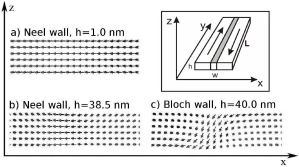
Figure 1: Néel and asymmetric Bloch domain walls, magnetization distribution in the $x$-$z$ plane. Sample (permalloy) is infinite along $y$, has thickness $h$ along $z$ and has width $w=200$ nm along $x$.

Despite its fundamental nature, it has been unclear whether the Néel to Bloch transition at $h_{c}$ is continuous or discontinuous.hubert:1975 ; metlov:2005 ; trunk:2001 A recent and comprehensive magnetostatics study by Kakay and Humphreykakay:2005 indicates that the transition between Néel walls and asymmetric Bloch walls is first order, although the authors were cautious in identifying the specific thickness at which the transition occurs.

The present Letter considers the nature of this transition (continuous or discontinuous) by extending our work on the staticsRivkinRomanov-Neel:2007 and dynamics for Néel and Bloch walls. We numerically studyrivkin:2004 the spectrum of normal modes as a function of the sample thickness $h$, and identify an unstable mode whose frequency vanishes at a critical thickness $h_{c}$. We numerically show that the ground state of samples with $h<h_{c}$ is a Néel domain wall and the ground state of samples with $h>h_{c}$ is an asymmetric Bloch wall.

We also show that the transition can be described analytically by a Landau theory of second order phase transitions with a single order parameter — the amplitude of the unstable mode. We derive the Landau free energy for the transition up to the fourth order in the order parameter. In agreement with the numerics, the frequency of the critical mode $\omega\sim\sqrt{h_{c}-h}$ just below the critical thickness.

Micromagnetics. Consider a ferromagnetic strip of thickness $h$ along $z$, width $2w$ along $x$, and infinite along $y$ (inset to Figure 1). We assume that the exchange length $l_{ex}=\sqrt{A/2\pi M_{s}^{2}}$ satisfies $l_{ex}\ll w$. Our samples are large enough for the domain wall center to completely fit within the sample. The material parameters chosen are appropriate to permalloy: exchange constant $A=1.30\times 10^{-6}$ erg/cm and saturation magnetization $M_{s}=795$ emu/cm³, which gives $l_{ex}=5.72$ nm. We take no crystalline anisotropy. The magnetization for $x=0$ is taken to be parallel to $x$-axis and free boundary conditions are taken on the sides of the strip.

The calculation of the spectrum for samples with different thicknesses started from thin samples $h$ (1–5 nm) and magnetization $\vec{m}_{i}^{0}=\hat{\vec{y}}M_{s}$, $x<0$, $\vec{m}_{i}^{0}=-\hat{\vec{y}}M_{s}$, $x\geq 0$. We equilibrated and then calculated the normal modes and their coupling to a uniform rf external magnetic field. Using this equilibrium as a starting point in the relaxation algorithm, we then gradually increased $h$ and calculated the new equilibrium configuration, normal modes, and rf couplings. We also started with large thicknesses and gradually decreased the thickness, to check for bi-stable solutions.

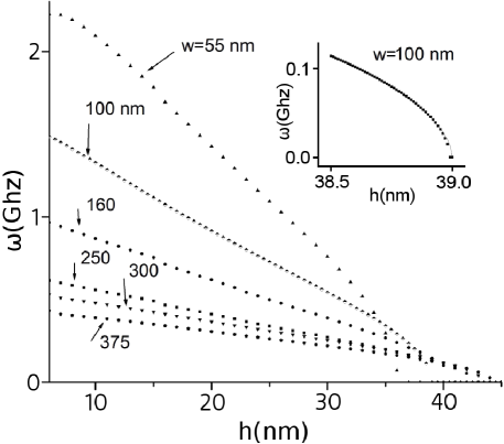
Figure 2: Frequency $\omega$ of the critical mode as a function of sample thickness $h$ for different half widths $w$. Inset: critical mode frequency near the critical thickness $h_{c}$, numerical results (dots) and square root fit (line) for $w=100$ nm.

The main two results of the micromagnetics calculations are: (1) The ground magnetization state for small thicknesses is indeed the Néel domain wall. In this system the Néel wall has three distinct regions — the central region of width $2\delta$ and logarithmic tails.RivkinRomanov-Neel:2007 (2) There is one mode of oscillations with frequency $\omega$ which goes to $0$ at some critical thickness $h_{c}$ (Fig 2). This mode approximately corresponds to a $z$-dependent oscillation of the domain wall core along $x$. The oscillations are confined to the central part of the Néel domain wall, whereas the logarithmic tails remain unperturbed. The frequency $\omega$ depends on both the width $2w$ and on the height $h$.

To a very good approximation, the (un-normalized) critical mode has in-plane oscillations of the form

$$m_{x}^{(1)}(x,z) \approx \text{Re}\left[\tanh\left(\frac{x}{\delta}\right)\text{sech}\left(\frac{x}{\delta}\right)e^{i\phi(x,z)-i\omega t}\right],$$ (1)

$$m_{y}^{(1)}(x,z) \approx \text{Re}\left[\text{sech}^{2}\left(\frac{x}{\delta}\right)e^{i\phi(x,z)-i\omega t}\right].$$ (2)

Here $\delta$ – the half-width of the domain wall center – was determined from a fit to the central region of the domain wall. The $x$-$y$ phase factor $\phi(x,z)$ determines the symmetry properties of the mode, but is not needed for the present purpose.

The out-of plane oscillations $m_{z}^{(1)}(x,z)$ have the form

$$m_{z}^{(1)}\approx\text{Re}\left[\text{sech}\left(\frac{x}{\delta}\right)\left(2\text{sech}\left(\frac{x}{\delta}\right)-1\right)e^{i\phi_{z}(x,z)-i\omega t}\right],$$ (3)

where the $z$ phase factor $\phi_{z}(x,z)$ differs from $\phi(x,z)$. The amplitude of the out-of-plane oscillations is typically less than 25% of the amplitude of the in-plane oscillations, except for $h$ near $h_{c}$.

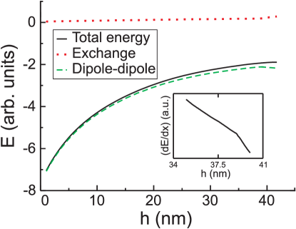
Figure 3: Magnetostatic energy and its first derivative as a function of thickness $h$ ($w=100$ nm).

The inset to Figure 2 shows, for $w$ = 100 nm, the thickness dependence of $\omega$ just below the critical thickness $h_{c}$ (dots) as well as a fit (line) confirming the $\sqrt{h_{c}-h}$ dependence. As $h$ increases above $h_{c}$, and ground state is taken as Néel wall, the imaginary part of $\omega$ goes from negative (stable) to positive (unstable). This is the only unstable mode.

Near $h_{c}$ conventional methods (conjugate gradient algorithm, Landau-Lifshitz equation in the presence of large damping, etc.) failed to find the equilibrium state. This is because among all the modes in the Néel state only one is unstable; therefore any random perturbation of the initial configuration will contain only a negligible projection on the unstable mode. Moreover, the unstable imaginary part of the eigenfrequency is of order 1000 Hz, which would require an enormous time interval for the instability to be observed by numerical integration. The only method we found to produce reliable and consistent results was to study the normal modes for the unstable initial configuration, find the unstable mode, and then add a component of an unstable eigenvector to the static solution. This led to a significant decrease of energy and gave a magnetization close enough to the true local equilibrium that more conventional methods then applied.

For $w=100$ nm the domain wall for $h>h_{c}$, where $h_{c}\approx 39$ nm, is indeed an asymmetric Bloch wall (Figure 1). Figure 3 shows that to numerical accuracy both the total magnetostatic energy and its derivative remains continuous through the transition, although the dipole-dipole and exchange energies individually have discontinuous first derivatives. The second derivative of the magnetostatic energy is slightly discontinuous at the transition, which implies a second order transition. The difference between this and previous work trunk:2001 may be due to the failure of conventional numerical methods at the transition. If the calculations are performed with a false equilibrium (metastability), then as the film gets thicker more modes become unstable. At some thickness the numerical method finally finds the true equilibrium; at this point the transition would appear to be sudden.

We also numerically studied the dependence of $h_{c}$ on the exchange length $l_{ex}=\sqrt{A/2\pi M_{s}^{2}}$ and the sample width $w$. By varying these parameters and later fitting the results to about 5% we find the best fit to be given by the form (Figure 4):

$$h_{c}=5.4l_{ex}^{0.914}w^{0.086}\mbox{.}$$ (4)

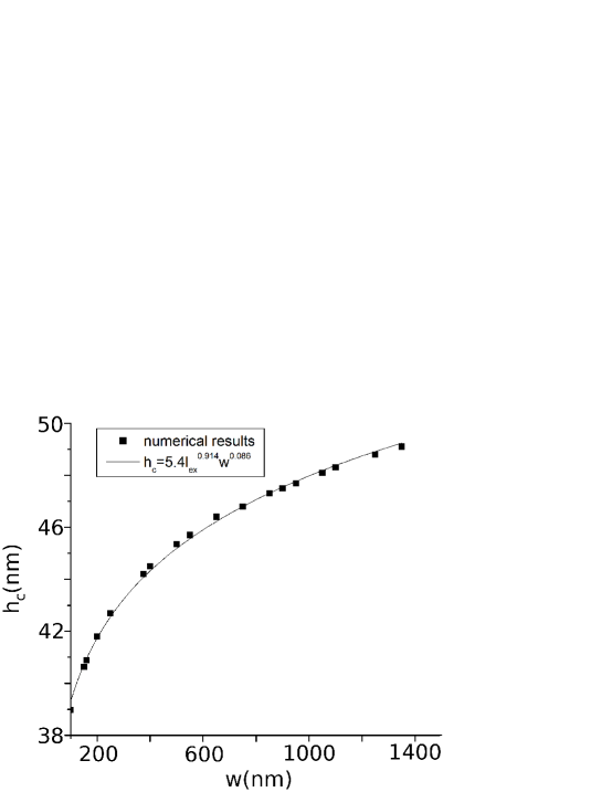
Figure 4: Critical thickness $h_{c}$ as function of width $w$: dots give numerical results; curve gives fit with (4).

Analytics. This section studies the symmetry properties of the transition mode and its corresponding state. It then relates the width $\delta$ of the Néel domain wall center and the thickness of the strip $h$ at the transition.

For very thin strips ($w\gg h$) below the critical thickness $h_{c}$ the stable magnetization configuration $\vec{M}^{0}(\vec{r})$ is a Néel domain wall (Fig.1b) with center at $x=0$ and parallel to the $z$-$y$ plane (Fig.1a). Because $h$ is very small $M^{0}_{z}$ is negligible, and $M^{0}_{x}$ and $M^{0}_{y}$ are nearly independent of $z$. (Due to translation invariance $\vec{M}$ does not depend on $y$.) Thus the most general Néel domain wall is

$$\vec{M}^{0}(\vec{r})={M_{s}}\hat{n}={M_{s}}(u(x),v(x),0)\mbox{,}$$ (5)

where $u(x)^{2}+v(x)^{2}=1$, subject to $u(\pm w)=0$, $v(\pm w)=\mp 1$, with $u(-x)=u(x)$ and $v(-x)=-v(x)$. For $\delta\ll w$, near the center of the domain wall, $u(x)\approx\text{sech}(x/\delta)$ and $v(x)\approx-\tanh(x/\delta)$.

Above the critical thickness $h_{c}$ the stable configuration is the asymmetric Bloch wall (Fig.1c), whose magnetization $\vec{M}^{B}(\vec{r})$ lacks the $x$ and $z$ reflection symmetries, but preserves inversion symmetry $(x,z)\rightarrow(-x,-z)$, $M^{B}_{x,z}(-x,-z)=M^{B}_{x,z}(x,z)$, $M^{B}_{y}(-x,-z)=-M^{B}_{y}(x,z)$.

The critical mode responsible for the Néel-to-asymmetric-Bloch-wall transition has magnetization $\vec{\mu}(x,z)=\vec{M}^{B}(x,z)-\vec{M}^{0}(x,z)$ and is symmetric under reflections of $x$ and $z$, so

$$\mu_{x}(-x,z)=-\mu_{x}(x,z);\qquad \mu_{x,y}(x,-z)=-\mu_{x,y}(x,z)$$ (6)

$$\mu_{y,z}(-x,z)=\mu_{y,z}(x,z);\qquad \mu_{z}(x,-z)=\mu_{z}(x,z)\mbox{.}$$

Since the amplitude of the critical mode is small, its magnetization is orthogonal to the static magnetization and can be written as

$$\vec{\mu}=M_{s}(\lambda(x,z)v(x),-\lambda(x,z)u(x),\zeta(x,z)),$$ (7)

where $\lambda(-x,z)=\lambda(x,z)$, $\lambda(x,-z)=-\lambda(x,z)$, $\zeta(x,z)=\zeta(x,z)$ and $\zeta(x,-z)=\zeta(x,z)$.

Expanding in small $z$ subject to the above symmetry conditions, with $\tilde{z}=2z/h$, we use the approximations

$$\lambda(x,z)=\left(\lambda_{1}\tilde{z}+\lambda_{3}\tilde{z}^{3}\right)f(x),\quad\zeta(x,z)=\left(\zeta_{0}+\zeta_{2}\tilde{z}^{2}\right)g(x),$$ (8)

where $\lambda_{0}$, $\lambda_{2}$, $\zeta_{1}$, and $\zeta_{3}$ are constants to be determined.

The micromagnetic calculations show that the critical mode is localized near the center of the strip and that it shifts the Néel domain wall core parallel to $x$. Thus $\mu_{x}(x,z)\sim\frac{d}{dx}M^{0}_{x}(x)$ and $\mu_{y}(x,z)\sim\frac{d}{dx}M^{0}_{y}(x)$. By comparison with the fits (1-3) to the micromagnetic calculations, a good set of approximations is

$$f(x)=\text{sech}\left(x/\delta\right),\,\,g(x)=\text{sech}\left(x/\delta\right)\left[2\text{sech}\left(x/\delta\right)-1\right].$$ (9)

The mode energy now takes the form

$$W_{m}[\hat{n},\vec{\mu}]=W_{ex}[\hat{n},\vec{\mu}]+W_{dd}[\hat{n},\vec{\mu}];$$ (10)

where $W_{ex}$ and $W_{dd}$ are the exchange and dipole-dipole contributions. Although the mode is localized in the central part of the domain wall, the exchange contribution to its energy is negligible, sohubert:2001

$$W_{m}[\hat{n},\vec{\mu}]=\int d\vec{r}_{1}d\vec{r}_{2}(\mu(\vec{r}_{1})\vec{\partial}_{r_{1}})(\mu(\vec{r}_{2})\vec{\partial}_{r_{2}})\frac{1}{|\vec{r}_{1}-\vec{r}_{2}|}.$$ (11)

We now expand the free energy functional using the trial solution (7-9). The energy of the mode is calculated to second order in the $\lambda_{i}$, $\zeta_{j}$, and by stability has no first-order terms. With the row vector $Z=\left(\lambda_{1},\lambda_{3},\zeta_{0},\zeta_{2}\right)$ and its column (transpose) vector $Z^{T}$, we have

$$W_{m}[\hat{n},\vec{\mu}]=Z\hat{W}_{mode}Z^{T},$$ (12)

where $\hat{W}_{mode}$ is a $4\times 4$ matrix whose elements depend on the system parameters.

At the critical thickness $h_{c}$ one of the eigenvalues of $\hat{W}_{mode}$ goes to zero, so its determinant goes to zero:

$$Det\,\hat{W}_{mode}=0.$$ (13)

For small exchange length $l_{ex}$, as we have here, $\hat{W}_{ex}\ll\hat{W}_{dd}$. The term $\hat{W}_{dd}$ is a function only of $\delta/h$. Solving (13) yields $h_{c}\approx 0.8\delta_{c}$ (to about 10%). (Here $\delta=\delta_{c}$ is evaluated at the transition.) This is in good agreement with the numerics, where for different $w$ and $l_{ex}$ we find $0.74<h_{c}/\delta_{c}<0.78$. The unnormalized critical vector is

$$Z_{c}=(0.19,0.70,0.66,0.17).$$ (14)

This yields the form of $\vec{\mu}(x,z)$; its amplitude is determined by a higher order expansion in the energy.

The smallest eigenvalue $\lambda_{0}$ of the matrix $\hat{W}_{mode}$ goes to zero linearly when $h$ approaches $h_{c}$. Because the rest of the modes have finite energy a standard result of Landau-Lifshitz equations is that the frequency of the mode $\omega^{2}\sim\lambda_{0}\sim h_{c}-h$, so that the frequency goes to zero at the critical thickness as a square root $\omega\sim\sqrt{h_{c}-h}$.

The expression (7) gives only the first order approximation to the transition mode $\vec{\mu}(x,z)$. The second order correction $\vec{\chi}(x,z)$ can be obtained from $|\vec{M}^{B}(x,z)|=|\vec{M}^{0}(x,z)+\vec{\mu}(x,z)+\vec{\chi}(x,z)|=M_{s}$ and $\vec{\mu}(x,z)\perp\vec{\chi}(x,z)$. Using this correction, one can calculate the free energy near the transition:

$$W_{mode}(\eta)=\eta^{2}0.3M_{s}^{2}Lh^{2}\left(\frac{\delta}{h}-\frac{\delta_{c}}{h_{c}}\right)+0.008\eta^{4}M_{s}^{2}Lh^{2},$$ (15)

where $\eta$ is the amplitude of the critical mode.

Because there is no $\eta^{3}$ term, the relation between $W_{mode}(h)$ and the mode frequency $\omega$ is:

$$\sqrt{2}\left.\frac{\partial\omega}{\partial h}\right|_{h=h_{c}-0}=-\left.\frac{\partial W_{mode}}{\partial h}\right|_{h=h_{c}+0}\,.$$

Summary and Discussion. Experimental study of the transition by measurement of the magnetization and even the critical mode would be desirable. Because the symmetry under $-z$ to $+z$ of the critical mode changes at the transition, from in-phase to out-of-phase, there are drastic symmetry changes in the absorption. Thus, whereas for $h<h_{c}$ (Néel wall) the mode strongly couples to a uniform out-of-plane rf field, for $h>h_{c}$ (asymmetric Bloch wall) it becomes anti-symmetric with respect to the z axis and cannot couple to this same rf field.

To summarize, we have found that the Néel to asymmetric Bloch wall transition in dipole-dipole coupled thin magnetic films of infinite length along one direction, with relatively large width $2w$, is a smooth function of thickness $h$. The normal mode frequencies reveal that at a critical thickness $h_{c}$ the frequency of the transition mode, where the nature of the domain wall changes, goes to zero as $\sqrt{h_{c}-h}$. To high accuracy, both static and dynamic calculations indicate that this transition is continuous, as also supported by analytical studies.

- (1) F. Bitter, Phys. Rev. 38, 1903-1905 (1931).
- (2) F. S. Bloch, Zeitschrift für Physik 74, 295-335 (1932).
- (3) L. D. Landau, and E. M. Lifshitz, Physik. Z. der Sowjetunion 8, 153–169 (1935).
- (4) L. Néel, Comptes Rendus Hebdomadaires des Séances de l’Académie des Sciences 421, 533-536 (1955).
- (5) S. Middlehoek, IBM J. Res. 10, 351-354 (1966).
- (6) M. R. Scheinfein, J. Unguris, R. J. Celotta, and D. T. Pierce, Phys. Rev. Lett. 63, 668-671 (1989).
- (7) M. R. Scheinfein, J. Unguris, J. L. Blue, K. J. Coakley, D. T. Pierce, R. J. Celotta, and P. J. Ryan, Phys. Rev. B 43, 3395–3422 (1991).
- (8) C. Melcher, Arch. Rat. Mech. Anal. 168, 83–113 (2003).
- (9) K. Rivkin, K. Romanov, Y. Adamov, Ar. Abanov, W. Saslow, and V. Pokrovsky, Phys. Rev. B (submitted to Phys. Rev. B).
- (10) C. C. Chang, Y. C. Chang, I. C. Lo, and J. C. Wu, J. Magn. Magn. Mat., 310, 2612–2614 (2007).
- (11) M. Redjdal, J. Giusti, M. F. Ruane, and F. B. Humphrey, J. Appl. Phys., 91, 7547–7549 (2002).
- (12) A. Hubert, IEEE Transactions on Magnetics 11, 1285–1290 (1975).
- (13) K. Metlov, J. Low Temp. Phys. 139, 207-219 (2005).
- (14) T. Trunk, M. Redjdal, A. Kakay, M. F. Raune, and F. B. Humphrey, J. Appl. Phys. 89, 7606–7608 (2001).
- (15) A. Kakay, Numerical investigations of micromagnetic structures, Research Institute for Solid State Physics and Optics, Hungarian Academy of Sciences (2005).
- (16) K. Rivkin, A. Heifetz, P. R. Sievert, and J. B. Ketterson, Phys. Rev. B 70, 184410 (2004).
- (17) A. Hubert, and R. Schafer, Magnetic Domains: The Analysis of Magnetic Microstructures, Springer (2001), p.148. Eq.(3.61).