Spine–sheath layer radiative interplay in subparsec–scale jets and the TeV emission from M87

Abstract

Simple one–zone homogeneous synchrotron self–Compton models have severe difficulties is explaining the TeV emission observed in the radiogalaxy M87. Also the site the TeV emission region is uncertain: it could be the unresolved jet close to the nucleus, analogously to what proposed for blazars, or an active knot, called HST–1, tens of parsec away. We explore the possibility that the TeV emission of M87 is produced in the misaligned subpc scale jet. We base our modelling on a structured jet, with a fast spine surrounded by a slower layer. In this context the main site responsible for the emission of the TeV radiation is the layer, while the (debeamed) spine accounts for the emission from the radio to the GeV band: therefore we expect a more complex correlation with the TeV component than that expected in one–zone scenarios, in which both components are produced by the same region. Observed from small angles, the spine would dominate the emission, with an overall Spectral Energy Distribution close to those of BL Lac objects with a synchrotron peak located at low energy (LBLs).

1 Introduction

An increasing number of extragalactic objects is detected at energies greater than 100 GeV. The list of published sources comprises 20 objects: as expected (e.g., Costamante & Ghisellini 2002), the bulk of them (17) belongs to the class of Highly Peaked BL Lac objects. In fact, the position of the synchrotron peak, usually located in (or close to) the X–ray band assures the existence, in these sources, of electrons with extremely large Lorentz factors ($\gamma=10^{5}$–$10^{6}$), a key ingredient for the emission in the TeV band via inverse Compton (IC) scattering. The remaining three sources are BL Lac itself, which belongs to the LBL class, (Albert et al. 2007), 3C279, a FSRQs, (Teshima et al. 2007) and the nearby (16 Mpc, Tonry 1991) radiogalaxy M87 (Aharonian et al. 2003, 2006).

Already suggested as a possible source of high-energy radiation (e.g. Bai & Lee 2001) based on its similarity with BL Lac objects (Tsvetanov et al. 1998), M87 was discovered as a TeV source by the HEGRA array of Cherenkov telescopes (Aharonian et al. 2003) and it has been recently confirmed by H.E.S.S. (Aharonian et al. 2006). Due to the limited spatial resolution it is not possible to identify the emission region of this radiation. However, the sensitivity of H.E.S.S. allowed the detection of variability on short timescales ($\sim$ days), suggesting a compact emission region.

Three main sites have been proposed as emission regions for the TeV radiation: the resolved jet (in particular the so–called knot HST–1); the unresolved base of the jet (in analogy with blazars); the vicinity of the supermassive ($M=3\times 10^{9}$ $M_{\odot}$, Marconi et al. 1997) black hole (BH).

HST–1 is a quite interesting jet feature located at 60 pc (projected) from the core of of M87. Superluminal motions with apparent speeds up to $\sim 6c$ were observed with HST (Biretta et al. 1999). Continuous multifrequency coverage has shown spectacular activity from this knot in the past years (Perlman et al. 2003; Harris et al. 2006, 2007; Cheung et al. 2007). In particular, the X–ray flux increases by a factor of $\sim 30$ from 2000 to 2005 and since then it is steadily decreasing. These variations are accompanied by similar changes in the optical and in the radio bands and by the appearance of new superluminal components. This extreme phenomenology is described by Stawarz et al. (2006) on the assumption that HST-1 marks the recollimation shock of the jet. As such, HST–1 is thought to be a rather efficient particle accelerator and thus a possible source of intense TeV radiation. However, the small variability timescales observed by H.E.S.S. put strong limits to the size of the source ($R<c\Delta t\,\delta\simeq 5\times 10^{15}\delta$ cm, where $\delta=[\Gamma(1-\beta\cos\theta)]^{-1}$ is the relativistic Doppler factor, $\theta$ is the viewing angle and $\Delta t\sim 2$ days), which seems difficult to accomplish in this scenario (e.g. Neronov & Aharonian 2007; Levinson 2007).

The rapid variability could be easily reproduced if the TeV emission is produced close to the base of the jet, in the region associated to the emission from blazars. However, standard one–zone leptonic models face difficulties in reproducing the observed spectral energy distribution (SED) of the core including the TeV data. A possible solution advocates that the emission comes from a decelerating jet (Georganopoulos et al. 2005) . Alternatively, the emission can be produced by high–energy protons (Reimer et al. 2004). Going further in towards the BH, TeV photons could be emitted through IC by relativistic pairs produced by electromagnetic cascades in the BH magnetosphere (Neronov & Aharonian 2007).

The determination of the site producing the high-energy emission is rather important. Indeed, if the emission site will be eventually identified as knot HST-1, this would have a broad impact on the current view of relativistic jets (see the discussion in Cheung et al. 2007). It is thus extremely important to investigate whether the standard view (or minimal variations of it) for the inner jet is able reproduce the observed phenomenology. If not, it would be mandatory to explore the other alternatives.

As discussed in Ghisellini, Tavecchio & Chiaberge (2005, hereafter Paper I), there is compelling evidence supporting the view that jets of BL Lac objects are structured at blazar scales (at distances $\sim 10^{17}$ cm from the BH), with a fast core (spine) surrounded by a slower sheet (layer). In Paper I we showed that the radiative coupling between the spine and the layer can naturally account for the deceleration inferred for the jet between the blazar and the VLBI scale. Furthermore, one component sees the radiation of the other boosted, since the relative velocity can be relativistic. This enhances the IC emission of both the spine and the layer.

A direct consequence of such a structure is that while at small viewing angle (as in the case of blazars) the emission is dominated by the boosted spine emission, at large observing angles ($\theta>45^{\circ}$, typical for radio–galaxies) the emission from the spine would be suppressed, while the layer, characterised by a broader beaming cone, could substantially contribute to (and sometimes dominate) the overall emission. At intermediate angles both components can significantly contribute. Following this line, in this letter we explore an alternative interpretation for the TeV emission of M87, assuming that the TeV radiation is produced in the layer of the misaligned jet. We use $H_{\rm 0}\rm=70\;km\;s^{-1}\;Mpc^{-1}$, $\Omega_{\Lambda}=0.7$, $\Omega_{\rm M}=0.3$.

2 The spine–layer scenario

2.1 Difficulties with the one–zone models

The SED of the core of M87 is reported in Fig. 1 (grey open points, see Paper I for references) together with the H.E.S.S. spectra for 2004 (open blue squares) and 2005 ( open red triangles) as reported by Aharonian et al. (2006). The X–ray spectrum (as observed in July 2000) is taken from Balmavarde, Capetti & Grandi (2006). Note that the slope [$\alpha=1.3\pm 0.1$; $F(\nu)\propto\nu^{-\alpha}$] is intermediate between that reported in Marshall et al. (2002) ($\alpha=1.47\pm 0.08$, see also Donato, Sambruna & Gliozzi 2004) and that of Wilson & Yang (2002) ($\alpha=1.17\pm 0.1$). The X–ray spectral shape was not determined in 2004 and 2005, and for simplicity we assume that it is the same of 2000, with a normalisation that is a factor 3 (2004, blue) and 4 (2005, red) greater. This reproduces the increase of the X–ray flux of the core recorded through the continuous monitoring of Chandra (Harris et al. 2007).

The data describe a bump peaking at $\sim 10^{14}$ Hz and extending into the X–ray band, while the TeV emission clearly belongs to a second component. The SED closely resembles that usually observed in blazars, in which the first component is synchrotron emission from relativistic electrons and the second peak is produced through IC emission (e.g., Ghisellini et al. 1998). For M87 there is no evidence of powerful sources of soft photons in the nucleus and hence the high–energy emission should be dominated by the Synchrotron self–Compton emission (SSC; e.g., Maraschi et al. 1992). However, a simple one–zone synchrotron–SSC model cannot easily describe the observed SED. The reason is that in order to have the synchrotron component peaking in the IR region ($\nu_{s}\simeq 10^{14}$ Hz) and the SSC one close to the TeV band ($\nu_{C}\simeq 10^{26}$ Hz, as required by the relatively flat TeV spectra) one is forced to assume a rather low magnetic field and an unreasonably large Doppler factor. Following Tavecchio, Maraschi & Ghisellini (1998) and defining the synchrotron and SSC peak luminosities, $L_{s}\equiv\nu_{s}L(\nu_{s})$ and $L_{C}\equiv\nu_{C}L(\nu_{C})$ and the variability timescale $\Delta t$, one obtains:

$$\delta\simeq 500\,L_{s,41.5}^{1/2}L_{C,40.5}^{-1/4}\,\nu_{s,14}^{-1}\,\nu_{C,26}^{1/2}\,\Delta t_{1d}^{-1/2}$$ (1)

Here $Q=10^{x}Q_{x}$, in cgs units, except for $\Delta t$, that is in days. The adopted numerical values are appropriate for M87.

This is a general problem faced by any synchrotron–SSC model using a single emission region. A direct way to overcome this problem is to “decouple” synchrotron and the IC components, assuming that the two components are produced by two different regions. Such a “two-zones” model would allow us to reproduce the low–frequency bump (emitted by electrons with relatively low energy) with one emission component and the TeV emission with a separate source with high–energy electrons. This opportunity is directly offered by the spine–layer scenario. In this case the debeamed spine (or, alternatively, the layer) could be responsible for the low–energy bump and the layer (or the spine) of the TeV component.

2.2 The model

We focus on the case of a sub–pc scale emission region, due to the observed inter–day variability of the TeV emission, difficult to explain if HST–1 is responsible for this emission.

We are aware that we are almost doubling the number of the free parameters (one set for the spine, one set for the layer), and therefore we pay the increased flexibility with an increased uncertainty concerning the value of the parameters themselves and a loss of predictive power. On the other hand, our main aim at this stage is not much to find whether/what specific physical conditions (value of the magnetic field, beaming factor, number of particles, and so on) are univocally determined by the model, but to show that one can attribute the radiation we see to the the sub–pc jet (with “minor” modification of the simplest model) without radically changing our ideas about the emission models of blazars. Having said that, we will nevertheless do our best to find the most reasonable set of parameters. This is why we will not only try to fit the SED of M87, but we will worry about what kind of blazar would M87 be if seen at small angles. If the resulting SED would be too odd with respect to the known blazar SED, we will discard the found parameter set.

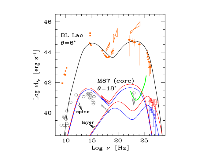
Figure 1: SED of the core of M87 (grey open points) together with the H.E.S.S. spectra taken in 2004 (open blue squares) and 2005 (open red triangles), from Aharonian et al. (2006). The grey bow–tie reports the X–ray spectrum as measured by Chandra in 2000 (from Balmaverde et al. 2006). We reproduced the increased X–ray emission of 2004 and 2005 assuming the same slope and a larger normalisation (blue and red bow–ties). The lines report the emission from the spine and from the layer for the two states as calculated with the parameters reported in Tab. 1. For comparison the green line indicates the sensitivity of GLAST ($5\sigma$, 1 year, converted in luminosity assuming the distance of M87). The upper black line reports the emission from the spine that would detect an observer located at an angle of 6^∘ from the jet axis (the corresponding emission from the layer is well below that of the spine and is not reported for semplicity). For comparison, we show the data of BL Lac (filled orange symbols, from Ravasio et al. 2002, TeV data from Albert et al. 2007). See text for details.

We refer to Paper I for a complete description of the model. Briefly, we assume that the jet comprises two regions: i) the spine, assumed to be a cylinder of radius $R$, height $H_{s}$ (as measured in the spine frame) and in motion with bulk Lorentz factor $\Gamma_{s}$; ii) the layer, modelled as an hollow cylinder with internal radius $R$, external radius $R_{2}$, height $H_{l}$ (as measured in the frame of the layer) and bulk Lorentz factor $\Gamma_{l}$. Each region is characterised by tangled magnetic field with intensity $B_{s}$, $B_{l}$ and it is filled by relativistic electrons assumed to follow a smoothed broken power–law distribution extending from $\gamma_{min}$ to $\gamma_{cut}$ and with indices $n_{1}$, $n_{2}$ below and above the break at $\gamma_{b}$. The normalisation of this distribution is calculated assuming that the system produces an assumed synchrotron luminosity $L_{syn}$ (as measured in the local frame), which is an input parameter of the model. As in Paper I we assume that $H_{l}>H_{s}$. The seed photons for the IC scattering are not only those produced locally in the spine (layer), but we also consider the photons produced in the layer (spine). Hereafter we will indicate this component as External Compton (EC).

To properly calculate the observed emission, it is necessary to take into account the different beaming patterns associated to the two emission components. This is because, in the comoving frame of the spine (layer), the photons produced by the layer (spine) are not isotropic, but are seen aberrated. Most of them are coming from almost a single direction (opposite to the relative velocity vector). In this case the produced EC is anisotropic even in the comoving frame, with more power emitted along the opposite direction of the incoming photons (i.e. for head–on scatterings). We therefore must take into account this anisotropy in the comoving frame when transforming in the observer frame. Consider also that this applies only to the EC radiation, while the synchrotron and the SSC emissions are isotropic in the comoving frame. The EC radiation pattern of the spine will be more concentrated along the jet axis (in the forward direction) with respect to its synchrotron and SSC emission. On the contrary, the EC radiation pattern of the layer will be less concentrated along the forward direction (with respect to its synchrotron and SSC) because, in the comoving frame, the layer emits more EC power in the backward direction (e.g. back to the black hole). The corresponding transformations are fully described in Paper I, and we briefly summarise them in the following. We here follow Dermer (1995), assuming that, due to the strong aberration, in the rest frame of the spine (layer) all the photons, assumed to be isotropic in the layer (spine) frame, can be considered as coming from a single direction, i.e. along (opposite to) the jet axis. This approximation greatly simplifies the calculations, allowing us not to consider the detail of the geometry in the transformations.

The beaming of the synchrotron and SSC emission for both regions follows the usual $\delta_{s}^{3+\alpha}$ (spine) and $\delta_{l}^{3+\alpha}$ (layer) pattern, while the patterns of the EC components are described by more complex shapes. In particular, the EC from the spine will have a rather narrow pattern given by $\delta_{s,l}^{4+2\alpha}\delta_{l}^{3+\alpha}$, where $\delta_{s,l}$ is the Doppler factor of the spine as measured in the layer frame. The first term ($\delta_{s,l}^{4+2\alpha}$) describes the same pattern as the EC radiation produced when scattering the seed photons produced by the broad line regions of powerful blazars, as firstly pointed out by Dermer (1995). It can be understood by going in the reference frame where the seed photons are isotropic (in this case this means comoving with the layer). In this frame we see the EC from the spine boosted by the “Dermer” pattern $\delta_{s,l}^{4+2\alpha}$. Finally, we go to the observer frame using the standard $\delta_{l}^{3+\alpha}$ term. Analogously, the amplification of the EC from the layer is $\propto\delta_{l,s}^{4+2\alpha}\delta_{s}^{3+\alpha}$. The net result is that the EC emission from the layer is less boosted in the observer frame than the corresponding EC emission from the spine.

Fig. 2 illustrates this point, showing the amplification factors of the different components as a function of the viewing angle (from 0^∘ to 45^∘), calculated assuming $\Gamma_{s}=12$ and $\Gamma_{l}=4$ (the values we used for M87, see below). Solid lines refer to the spine, dashed lines to the layer. Black and red lines correspond to the synchrotron/SSC and EC amplification factors, respectively. For the spine, the EC amplification is larger than the Synchrotron/SSC one for small angles, while at large angles the latter dominates. In this sense one can say that the EC emission has a narrower pattern than the Synchrotron/SSC emission. The opposite occurs for the layer: at small angles the synchrotron/SSC amplification is larger then the EC one, which instead becomes more important at large angles. Note, moreover, that the EC/layer emission has its maximum at $\simeq$10^∘, while all the other curves peak at 0^∘. To understand this, consider the emission pattern in the frame comoving with the layer. In this frame the seed photons produced by the spine are coming along the black hole–layer direction: as a consequence the relativistic electrons will produce more EC radiation in the opposite (layer–black hole) direction. This is the radiation that will be boosted the least when we transform the intensity in the observer frame (and the opposite for radiation along the outward radial direction: in the comoving frame it is the weakest, but it is boosted the most when going to the observer frame). This “compensation” between the intrinsic anisotropy as seen in the comoving frame and the beaming effect means that the maximum flux will be observed not at 0^∘, but at a larger angle. At the extreme, if the layer is not moving, the maximum will be observed at 180^∘. This characteristic is particularly relevant for sources seen at large angles: for those, the EC produced by the layer becomes relatively more important.

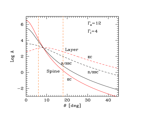
Figure 2: Amplification factors for the different emission components as a function of the viewing angle. Solid (dashed) lines refer to the spine (layer), while black (red) lines show the to synchrotron/SSC (EC) factors. We assume $\Gamma_{s}=12$ and $\Gamma_{l}=4$, the values we used for the case of M87, and $\alpha=1$. The two vertical lines indicate the two angles assumed for the calculation of the SEDs, $6^{\circ}$ and $18^{\circ}$. See text for discussion.

2.3 Results

We have two possibilities to reproduce the SED with this model: i) either we assume that the low energy bump is produced by the layer and the TeV emission originates in the spine or ii) the layer produces the TeV radiation and the spine mainly contributes at low frequencies. The first choice is disfavoured in the present case. In fact, to produce TeV photons, the typical Lorentz factor of the electrons in the spine must be large ($\gamma\sim 10^{6}$) and, assuming typical magnetic fields of order 0.1–1 G, the corresponding synchrotron emission would peak in the hard X–ray band. Under this conditions the SSC emission would be deeply in the Klein–Nishina regime and thus strongly depressed and the TeV emission would be dominated by the EC component. If the spine SED is dominated by the EC component at large (18^∘) angles, it will be even more so at small angles (see Fig. 2), with $L_{\rm TeV}/L_{\rm X}\gg 20$. Instead, in TeV BL Lacs, the synchrotron and the IC components show comparable luminosities [with few exception, most notably 1ES 1426+428 (Aharonian et al. 2002), although the TeV luminosity depends on the still unclear amount of intergalactic absorption]. On the other hand, as we show below, the choice ii) leads to a predicted SED for the beamed counterpart of M87 closely resembling those observed in LBL sources and thus we decided to adopt this view in the modelling.

	$R$	$H$	$L_{\rm syn}$	$B$	$\gamma_{\rm min}$	$\gamma_{\rm b}$	$\gamma_{\rm cut}$	$n_{1}$	$n_{2}$	$\Gamma$	$\theta$
	cm	cm	erg s-1	G							deg.
spine low	7.5e15	3e15	4.0e41	1	600	5e3	1e8	2	3.7	12	18
layer low	7.5e15	6e16	1.6e38	0.35	1	2e6	1e9	2	3.7	4	18
spine high	7.5e15	3e15	5.2e41	1	600	5e3	1e8	2	3.7	12	18
layer high	7.5e15	6e16	4.0e38	0.2	1	6e6	1e9	2	3.7	4	18

Table 1: Input parameters of the models for the layer and the spine shown in Fig. 1. All quantities (except the bulk Lorentz factors $\Gamma$ and the viewing angle $\theta$) are measured in the rest frame of the emitting plasma. The external radius of the layer is fixed to the value $R_{2}=1.2\times R$. The corresponding values of the electron density are: 108.3 cm^-3 and 140.8 cm^-3 (spine low and high); 0.74 cm^-3 and 2.04 cm^-3 (layer low and high).

The SEDs obtained for the core of M87 with the model are shown in Fig. 1 for both 2004 and 2005 and the parameters are reported in Table 1.

The model shown is intended as an example of the possible parameters giving a reasonable shape for the SED. A whole family of acceptable solutions, each one with different values for the parameters, is allowed. However, the joint request to reproduce the data and to have a spine SED resembling that of a BL Lac at small angles provides some constraints. Since the layer has to produce TeV radiation, the Lorentz factor of the electrons at the peak is constrained to be of the order of $\gamma_{b}\approx 10^{6}$, independently on the component (SSC or EC) dominating the high–energy emission. This, in turn, fixes the peak of the synchrotron component close to or within the X–ray band for the chosen magnetic field. Smaller $B$–values are allowed, but not larger, since in this case the layer synchrotron emission would overproduce the observed data. For the spine, as already discussed, most of the constraints come from the request that the Lorentz factor, the size and the magnetic field are similar to those typically inferred for (LBL) blazars.

The model slightly overproduces the emission in the optical band. However, since the optical and the X–ray emission are clearly correlated (Perlman et al. 2003) we expect that high X-ray fluxes correspond to high optical states. Note also that we predict quite bright GeV emission in this period, exceeding the EGRET upper limit by a factor of 3 and easily detectable with GLAST. The high-energy component of the layer is dominated by the EC emission from the beamed (in the layer frame) IR-optical photons from the spine. On the other hand, since the synchrotron component of the layer peaks in the X–rays, the EC emission of the spine is strongly suppressed by the effect of the Klein–Nishina cross section and hence the high–energy component is mainly SSC. The variability of the TeV flux from 2004 to 2005 is reproduced by increasing the luminosity radiated by the layer (and thus the corresponding density of the electrons) and slightly decreasing the magnetic field. Note also that the small size of the emitting region allows the rapid changes such as those detected by H.E.S.S. ($\Delta t\sim 2$ days).

A supplementary contribution to the IC emission from both the spine and the layer could come from the scattering of the external IR radiation field, possibly associated to the putative low–efficiency accretion flow. The luminosity of the core of M87 in the infrared band is $L\approx 10^{41}$ erg s^-1 (Perlman et al. 2001). This is an upper limit to the luminosity of the accretion flow, since the observed power law spectrum supports the idea that it is mainly associated to the emission from the jet (Perlman et al. 2001). We can set an upper limit to the importance of this component by assuming $L=10^{41}$ erg s^-1 for the accretion luminosity, produced in a region whose size is of the order the distance of the active region of the jet (around $\sim 10^{17}$ cm). This maximizes the importance of this external component: for smaller radii the accretion IR radiation would be strongly deboosted in the jet frame, while for larger radii it will be more diluted. Even so, this external component has a radiation energy density smaller (by more than an order of magnitude) of the one already present in the spine and in the layer.

Inspection of Fig. 1 reveals that we nicely reproduce the slope of the 2004 TeV spectrum, while the 2005 spectrum appears to be harder than the model (although the relatively large error bars prevent a firm conclusion). The steep slope of the model continuum in this band is the result of the $\gamma\gamma$ absorption of TeV photons interacting with optical–IR photons of the spine and thus cannot be simply avoided.

In Fig. 1 we also report (black line) the emission from the spine relative to 2004 as would appear to an observer almost aligned ($\theta=6^{\circ}$) with the jet. For comparison we report (orange, filled symbols) the multifrequency SED for BL Lac itself (the prototype of BL Lac objects), collected during different campaigns (see Ravasio et al. 2002 for references) and reporting also the TeV spectrum recently detected by MAGIC (Albert et al. 2007).

3 Discussion

We propose that the TeV emission detected from M87 originates in the structured jet at blazar scale. The most likely possibility is that the emission from the spine reproduces the low energy component, from radio to X–rays, while the layer contributes to the bulk of the TeV radiation. With this choice, the beamed counterpart of M87 observed at small angle would have a SED closely resembling those of Low–Peaked BL Lac objects. Correspondingly the spine is characterised by physical parameters close to those usually inferred for those sources ($\gamma_{b}\sim 10^{3}$, $B\sim 1$ G). The layer, instead, would be characterised by a low magnetic field ($B\sim 0.1$ G) and large peak Lorentz factors ($\gamma_{b}\sim 10^{6}$). It is possible that particles in the layer are energized by turbulent acceleration (e.g. Stawarz & Ostrowski 2002). In this case the expected distribution would have a pile-up at the energy where acceleration and loss processes are in equilibrium (e.g. Katarzynski et al. 2006). Suggestively, in our conditions (losses dominated by IC) the expected equilibrium Lorentz factor would be close to $\gamma\sim 10^{6}$ for $B\sim 0.1$ G.

Note that our conclusions are rather different from that of Georganopoulos et al. (2005) who discussed a similar model relying on the possibility that the jet experiences a strong deceleration at the blazar scale. In their model the high-energy emission is produced in the innermost and faster portion of the jet, while the slow external portions mainly contributes at low frequency. Under these conditions the beamed counterpart of M87 would be a TeV BL Lac. However, due to the different beaming patterns or the synchrotron and IC components (analogously to our case), the resulting spectrum would be characterised by a strong dominance of the TeV component with respect to the X–ray one, contrary to what is usually observed in the known TeV BL Lacs.

In our model the optical and the X–rays are produced by a region different from that responsible for the TeV emission. Therefore a strict correlation between low energy and TeV emission is not directly required (even if it is possible). Analogously, the MeV-GeV emission should originate in the spine. Therefore we expect that the emission possibly detected by GLAST will not exactly follow the TeV component.

A potential weak point of our model concerns the slope of the TeV spectrum. The slope is mainly dictated by the absorption of TeV photons by the dense optical radiation field and, in this sense, it is rather robust and does not strongly depend on the underlying slope of the intrinsic TeV spectrum. In particular, hard spectra such as that recorded in 2005 are quite difficult to achieve in this scheme. A possibility to avoid important absorption of gamma-rays would be to enlarge the emission region, hence diluting the target photon density and decreasing the absorption optical depth. However the increase of the source size is limited by the observed short variability timescales. Further observations with increased sensitivity could provide stringent constraints to our interpretation.

References

- [\citeauthoryearAharonian et al.2006] Aharonian F., et al., 2006, Science, 314, 1424
- [\citeauthoryearAharonian et al.2003] Aharonian F., et al., 2003, A&A, 403, L1
- [\citeauthoryearAharonian et al.2002] Aharonian F., et al., 2002, A&A, 384, L23
- [] Albert, J. et al., 2007, ApJ, 666, L17
- [\citeauthoryearBai & Lee2001] Bai J. M., Lee M. G., 2001, ApJ, 549, L173
- [\citeauthoryearBalmaverde, Capetti, & Grandi2006] Balmaverde B., Capetti A., Grandi P., 2006, A&A, 451, 35
- [\citeauthoryearBiretta, Sparks, & Macchetto1999] Biretta J. A., Sparks W. B., Macchetto F., 1999, ApJ, 520, 621
- [\citeauthoryearCheung, Harris, & Stawarz2007] Cheung C. C., Harris D. E., Stawarz Ł., 2007, ApJ, 663, L65
- [\citeauthoryearCostamante & Ghisellini2002] Costamante L. & Ghisellini G., 2002, A&A, 384, 56
- [\citeauthoryearDermer1995] Dermer C. D., 1995, ApJ, 446, L63
- [\citeauthoryearDonato, Sambruna, & Gliozzi2004] Donato D., Sambruna R. M., Gliozzi M., 2004, ApJ, 617, 915
- [\citeauthoryearGeorganopoulos, Perlman, & Kazanas2005] Georganopoulos M., Perlman E. S., Kazanas D., 2005, ApJ, 634, L33
- [\citeauthoryearKatarzynski, Ghisellini, Mastichiadis, Tavecchio & Maraschi] Katarzynski K., Ghisellini G., Mastichiadis A., Tavecchio F. & Maraschi L., 2006, A&A, 453, 47
- [\citeauthoryearGhisellini, Tavecchio, & Chiaberge2005] Ghisellini G., Tavecchio F., Chiaberge M., 2005, A&A, 432, 401 (Paper I)
- [\citeauthoryearGhisellini et al.1998] Ghisellini G., Celotti A., Fossati G., Maraschi L., Comastri A., 1998, MNRAS, 301, 451
- [\citeauthoryearHarris et al.2007] Harris D. E. et al. 2007, To appear in the proc. of ”Extragalactic Jets: Theory and Observation from Radio to Gamma Ray” ASP Conference Series, (arXiv:0707.3124)
- [\citeauthoryearHarris et al.2006] Harris D. E., Cheung C. C., Biretta J. A., Sparks W. B., Junor W., Perlman E. S., Wilson A. S., 2006, ApJ, 640, 211
- [\citeauthoryearMaraschi, Ghisellini, & Celotti1992] Maraschi L., Ghisellini G., Celotti A., 1992, ApJ, 397, L5
- [\citeauthoryearMarconi et al.1997] Marconi A., Axon D. J., Macchetto F. D., Capetti A., Soarks W. B., Crane P., 1997, MNRAS, 289, L21
- [\citeauthoryearMarshall et al.2002] Marshall H. L., Miller B. P., Davis D. S., Perlman E. S., Wise M., Canizares C. R., Harris D. E., 2002, ApJ, 564, 683
- [] Neronov A. & Aharonian F., 2007, ApJ submitted (arXiv:0704.3282)
- [\citeauthoryearPerlman et al.2003] Perlman E. S., Harris D. E., Biretta J. A., Sparks W. B., Macchetto F. D., 2003, ApJ, 599, L65
- [\citeauthoryearPerlman et al.2001] Perlman E. S., Sparks W. B., Radomski J., Packham C., Fisher R. S., Piña R., Biretta J. A., 2001, ApJ, 561, L51
- [\citeauthoryearRavasio et al.2002] Ravasio M., et al., 2002, A&A, 383, 763
- [\citeauthoryearReimer, Protheroe, & Donea2004] Reimer A., Protheroe R. J., Donea A.-C., 2004, A&A, 419, 89
- [\citeauthoryearStawarz et al.2006] Stawarz Ł., Aharonian F., Kataoka J., Ostrowski M., Siemiginowska A., Sikora M., 2006, MNRAS, 370, 981
- [\citeauthoryearStawarz & Ostrowski2002] Stawarz Ł., Ostrowski M., 2002, ApJ, 578, 763
- [\citeauthoryearTavecchio, Maraschi, & Ghisellini1998] Tavecchio F., Maraschi L., Ghisellini G., 1998, ApJ, 509, 608
- [\citeauthoryearTeshima1991] Teshima, M. et al. 2007, to appear in the proceedings of the 30th International Cosmic Ray Conference, Merida, July 2007 (arXiv:0709.1475)
- [\citeauthoryearTonry1991] Tonry J. L., 1991, ApJ, 373, L1
- [\citeauthoryearTsvetanov et al.1998] Tsvetanov Z. I., Hartig G. F., Ford H. C., Dopita M. A., Kriss G. A., Pei Y. C., Dressel L. L., Harms R. J., 1998, ApJ, 493, L83
- [\citeauthoryearWilson & Yang2002] Wilson A. S., Yang Y., 2002, ApJ, 568, 133