Distributed Power Allocation Strategies for Parallel Relay Networks

Abstract

We consider a source-destination pair assisted by parallel regenerative decode-and-forward relays operating in orthogonal channels. We investigate distributed power allocation strategies for this system with limited channel state information at the source and the relay nodes. We first propose a distributed decision mechanism for each relay to individually make its decision on whether to forward the source data. The decision mechanism calls for each relay that is able to decode the information from the source to compare its relay-to-destination channel gain with a given threshold. We identify the optimum distributed power allocation strategy that minimizes the total transmit power while providing a target signal-to-noise ratio at the destination with a target outage probability. The strategy dictates the optimum choices for the source power as well as the threshold value at the relays. Next, we consider two simpler distributed power allocation strategies, namely the passive source model where the source power and the relay threshold are fixed, and the single relay model where only one relay is allowed to forward the source data. These models are motivated by limitations on the available channel state information as well as ease of implementation as compared to the optimum distributed strategy. Simulation results are presented to demonstrate the performance of the proposed distributed power allocation schemes. Specifically, we observe significant power savings with proposed methods as compared to random relay selection.

I Introduction

Relay-assisted transmission schemes for wireless networks are continuing to flourish due to their potential of providing the benefits of space diversity without the need for physical antenna arrays [1]. Among the earliest work on cooperative networks are references [2, 3, 4]. A cooperative diversity model is proposed in [2] and [3], in which two users act as partners and cooperatively communicate with a common destination, each transmitting its own bit in the first time interval and the estimated bit of its partner in the second time interval. In [4], several low-complexity cooperative protocols are proposed and studied, including fixed relaying, selection relaying and incremental relaying, in which the relay node can either amplify-and-forward (AF) or decode-and-forward (DF) the signal it receives. In [5], networks consisting of more than two users that employ the space-time coding to achieve the cooperative diversity are considered. Coded cooperation schemes are discussed in [6] and [7], where a user transmits part of its partner’s codeword as well. References [8] and [9] investigate the capacity of relay networks of arbitrary size. References so far have shown that, relay nodes can provide performance improvement in terms of outage behavior [4, 5], achievable rate region[2, 3, 8, 9], and error probability [6, 7, 10, 11].

Power efficiency is a critical design consideration for wireless networks such as ad-hoc and sensor networks, due to the limited transmission power of the (relay and the source) nodes. To that end, choosing the appropriate relays to forward the source data, as well as the transmit power levels of all the nodes become important design issues. Optimum power allocation strategies for relay networks are studied up-to-date for several structures and relay transmission schemes. Three-node models are discussed in [12] and [13], while multi-hop relay networks are studied in [14, 15, 16]. Relay forwarding strategies for both AF and DF parallel relay channels in wideband regime are proposed in [17]. Recent works also discuss relay selection algorithms for networks with multiple relays. Optimum relay selection strategies for several models are identified in [10, 17, 18]. Recently proposed practical relay selection strategies include pre-select one relay [19], best-select relay [19], blind-selection-algorithm [20], informed-selection-algorithm [20], and cooperative relay selection [21]. All of these proposed methods result in power efficient transmission strategies. However, the common theme is that, the implementations of these algorithms require either the destination or the source to have substantial information about the network, such as the channel state information (CSI) of all communication channels, received signal-to-noise ratio (SNR) at every node, the topology of the network, etc. Such centralized power allocation/relay selection schemes may be infeasible to implement due to the substantial feedback requirements, overhead and delay they may introduce.

To overcome the obstacles of a centralized architecture, several heuristic approaches have been proposed in [22], for multi-user networks with coded cooperation. In this work, users select cooperation partners based on a priority list in a distributed manner. Although the proposed algorithms are advantageous due to their ease of implementation, their performance depends on the fading conditions, and the randomness in the channel may prevent the protocols from providing full diversity. In [23], an SNR threshold method is proposed for the relay node to make a decision on whether to forward the source data in a three-node model. Since there is only one relay node in the considered system, relay selection is not an issue. Reference [24] provides a relay selection algorithm based on instantaneous channel measurements done by each relay node locally. For the purpose of reducing the communication among relays, a flag packet is broadcasted by the selected relay to notify the other relays of the result.

In this paper, we investigate optimum distributed power allocation strategies for decode-and-forward parallel relay networks, in which only partial CSI is accessible at the source and the relay nodes. We first propose a distributed decision mechanism for each relay node to individually make a decision on whether to forward the source data. In contrast to the SNR based decision protocol presented in [23], in our proposed decision mechanism, the relay makes its decision not only by considering its received SNR, but also by comparing its relay-to-destination channel gain with a given threshold, and no feedback from the destination is needed. The overall overhead is further reduced as compared to the method proposed in [24] since the distributed decision mechanism does not require communication among relays. Secondly, given such a relay decision scheme, and considering an outage occurs whenever the SNR at the destination is lower than the required value (target), we formulate the distributed power allocation problem that aims to minimize the expected value of the total transmit power while providing the target SNR at the destination with an outage probability constraint. We identify the solution of this problem, that consists of the optimum value of the source power, and the corresponding relay decision threshold based on the partial CSI available at the source. The extra power the distributed power allocation mechanism needs as compared to the optimum centralized power allocation mechanism, i.e., the additional power expenditure, is examined to observe the tradeoff between the outage probability and the additional power expenditure.

We next consider two special cases with simpler implementation, namely the passive source model where the source does not contribute to the relay selection process, and the single relay model where one relay node is selected to forward the source data based on limited CSI. For each case, we optimize the respective relevant parameters. Our results demonstrate that considerable power savings can be obtained by our proposed distributed relay selection and power allocation schemes with respect to random relay selection.

The organization of the paper is as follows. In Section II, the system model is described. The distributed power allocation problem is formulated and the optimum solution is given in Section III. In Section IV, we investigate the passive source model and the single relay model. Numerical results supporting the theoretical analysis are presented in Section V, and Section VI concludes the paper.

II System Model and Background

We consider a relay network consisting of a source-destination pair and $N$ relay nodes employing decode-and-forward. We assume that the relay nodes operate in pre-assigned orthogonal channels, e.g. in non-overlapping time/frequency slots, or using orthogonal signatures. The source is assumed to transmit in a time slot prior to (and non-overlapping with) the relays. Let $f_{i}$ and $g_{i}$ denote the fading coefficients of the source-to-relay and relay-to-destination channels for the $i\mbox{th}$ relay node, for $i=1,...,N$. The fading coefficient of the source-to-destination link is denoted by $h$. We assume that each channel is flat fading, and $f_{i}$, $g_{i}$ and $h$ are all independent realizations of zero mean complex Gaussian random variables with variances $\sigma_{f_{i}}^{2}$, $\sigma_{g_{i}}^{2}$ and $\sigma_{h}^{2}$ per dimension, respectively.

Figure 1: Relay network system model.

Without loss of generality, we will assume that we have a time slotted system in the sequel. The system model is shown in Figure 1. In the first time slot, the source broadcasts $X_{o}$ with power $P_{s}$. The destination observes $y_{d_{0}}$:

$$y_{d_{0}}=\sqrt{P_{s}}hX_{o}+z_{d_{0}}$$ (1)

and the $i$th relay observes $y_{r_{i}}$:

$$y_{r_{i}}=\sqrt{P_{s}}f_{i}X_{o}+z_{r_{i}}~{}~{}~{}\mbox{for}~{}~{}i=1,...,N$$ (2)

where $z_{d_{0}}$ and $\{z_{r_{i}}\}_{i=1}^{N}$ are Additive White Gaussian Noise (AWGN) terms at the destination and the relays, respectively. Assume without loss of generality that they are of variance $1/2$ per dimension. The $i$th relay node is said to be reliable and can correctly decode $X_{o}$ when its received SNR, $SNR_{r_{i}}$, satisfies

$$SNR_{r_{i}}=P_{s}\left|f_{i}\right|^{2}\geq{SNR_{target}}$$ (3)

where ${SNR_{target}}$ is the given decodability constraint. In the subsequent time slots following the first one, the relays that belong to the set of reliable relays, $A_{R}$, can decode and forward the source data to the destination, each in its assigned time slot. Throughout this paper, we assume that the reliable relays simply regenerate the source data $X_{o}$ [4, 13, 15]. The signal received at the destination from the reliable relay $i$ is

$$y_{d_{i}}=\sqrt{P_{i}}g_{i}X_{o}+z_{d_{i}},~{}~{}~{}~{}~{}~{}i\in A_{R}$$ (4)

where $P_{i}$ is the transmit power of the $i$th relay node, and $z_{d_{i}}$ is the AWGN term at the $i$th relay-to-destination channel. The destination combines signals received from the reliable relay nodes and the direct link with a maximum ratio combiner (MRC), and the resulting SNR at the destination is

$${SNR}_{d}=P_{s}\left|h\right|^{2}+\sum_{i\in A_{R}}P_{i}\left|g_{i}\right|^{2}$$ (5)

We consider that the destination can correctly receive the source data whenever ${SNR_{d}}\geq{SNR_{target}}$.

Given this system model, the power allocation problem for regenerative DF relay networks with parallel relays can be posed as

$$\underset{Ps,\{P_{i}\}}{\min} P_{s}+\sum_{i\in A_{R}}P_{i}$$ (6)

s. t. $$P_{s}\left|h\right|^{2}+\sum_{i\in A_{R}}P_{i}\left|g_{i}\right|^{2}\geq{SNR_{target}}$$ (7)

$$P_{s}\left|f_{i}\right|^{2}\geq{SNR_{target}}~{}~{}\text{ for each}~{}i\in A_{R}$$ (8)

We note that the resulting power allocation strategy may prevent some reliable relays from participating simply by assigning zero power to those relays.

The optimum power allocation strategy for DF relay networks using different code books at the relays is identified in [17]. This strategy, re-stated below for the benefit of the reader, is easily seen to be the optimum centralized power allocation strategy for regenerative DF relay networks as well.

$$P_{s}^{*} = \frac{{SNR_{target}}}{\left|f_{k^{*}}\right|^{2}}$$ (9)

$$P_{i}^{*} = \left\{\begin{array}[]{ll}\left(\frac{{SNR_{target}}-\left|h\right|^{2}{SNR_{target}}/\left|f_{k^{*}}\right|^{2}}{\left|g_{k^{*}}\right|^{2}}\right)^{+},~{}i=k^{*}\\ 0,\text{otherwise}\end{array}\right.$$ (12)

$$k^{*} = \arg\underset{\{k\in A_{E}\}}{\min}\left[\frac{1}{\left|f_{k}\right|^{2}}+\frac{1}{\left|g_{k}\right|^{2}}-\frac{\left|h\right|^{2}}{\left|f_{k}\right|^{2}\left|g_{k}\right|^{2}}\right]$$ (13)

where $(\cdot)^{+}=\max(0,\cdot)$. In (13), the set $A_{E}$ denotes the set of efficient relays such that the transmission through the relay is more power efficient than the direct transmission, i.e.,

$$A_{E}={\{i|(\left|f_{i}\right|^{2}\geq|h|^{2})\cap(\left|g_{i}\right|^{2}\geq|h|^{2}),i=1..N\}}$$ (14)

Observe that when the source power is assigned as in (9), the relay node $k^{*}$, chosen according to (13), is the only relay node with received SNR equal to $SNR_{target}$. Thus, each relay node can decide whether it is the intended relay node by simply checking its received SNR. When the SNR contribution of the relay node, ${{SNR_{target}}-\left|h\right|^{2}{SNR_{target}}/\left|f_{k^{*}}\right|^{2}}$, is indicated explicitly by the source, the intended relay node can calculate its required transmit power as in (12) and forward $X_{o}$ to the destination. Alternatively, the source can broadcast the selected relay and the optimum power level in a side channel.

A moment’s thought reveals that to implement the strategy given by (9)-(13), the full CSI, i.e., $\{f_{i},g_{i}\}_{i=1}^{N}$ and $h$, at the source node, and the individual CSI, i.e., $\{f_{i},g_{i}\}$, at relay node $i$ are needed. Although (9)-(13) provides the most power efficient DF relay transmission strategy, its centralized nature, i.e., the fact that it requires the channel estimate of each link and the feedback of this information to the source, may render its implementation impractical. As such, distributed strategies are needed. In the following, we devise efficient distributed power allocation strategies.

III Distributed Power Allocation

Our aim in this paper is to find power allocation schemes that do not require a centralized mechanism, and utilize the limited available CSI at each node. In practice, it is feasible that the channels are estimated by training before the actual data transmission, when each node operates in TDMA mode. When the source transmits the training bits, all relay nodes can simultaneously estimate their source-to-relay fading coefficients $\{f_{i}\}_{i=1}^{N}$ due to the broadcast nature of the wireless medium. Similarly, when the relay node $i$ transmits the training bits, the source-to-relay coefficient $f_{i}$ can be estimated at the source. However, for $\{g_{i}\}_{i=1}^{N}$ to be available at the source, the feedback from the destination for each realization is required, which may be impractical. Thus, we investigate distributed power allocation schemes when the source has the realizations $\{f_{i}\}_{i=1}^{N}$ and $h$, and only the statistics of $\{g_{i}\}$. The relay nodes are assumed to have their individual CSI, i.e., $f_{i}$ and $g_{i}$ for relay $i$, $i=1,...,N$.

III-A Distributed Decision Mechanism

We first derive a distributed decision mechanism with the model assumptions given above. Since the source has only the statistical description instead of the realizations $\{g_{i}\}_{i=1}^{N}$, the optimum centralized power allocation indicated by (9)-(13) cannot be implemented by the source. Also, while it is clear that for a fixed source power, the best strategy is transmitting through the reliable relay node that has the highest relay-to-destination channel gain, this mechanism requires a comparison of all $\{g_{i}\}_{i=1}^{N}$. The distributed nature of the strategy requires that each relay should make its decision relying only on its individual CSI. Since each relay can easily determine whether it is a reliable relay by using its SNR value, i.e., its individual CSI, we propose that the $i$th reliable relay decides it will be a forwarding node when its channel gain to the destination satisfies

$$\left|g_{i}\right|^{2}\geq\gamma$$ (15)

where $\gamma$ is a given threshold value. Relay $i$ then forwards the decoded signal with sufficient power. That is, we have

$$P_{i}^{\ast}=SNR^{\prime}_{target}/{\left|g_{i}\right|^{2}}$$ (16)

where $SNR^{\prime}_{target}=(SNR_{target}-P_{s}|h|^{2})^{+}$ denotes the SNR contribution from the relay.

We note that such a distributed decision mechanism includes the probability that more than one relay will transmit. Similarly, we note that with any $\gamma>0$, the scheme results in a nonzero probability that none of the relay nodes satisfies (15), and hence a nonzero outage probability $\text{Prob}(SNR_{d}<SNR_{target})$. As such, the source should determine the optimum source power and the corresponding threshold $\gamma$ by considering the realizations of $\{f_{i}\}$ and the randomness in $\{g_{i}\}$, to meet a system given specification, i.e., an outage probability requirement.

III-B Source Power Allocation and Threshold Decision

Given the above described strategy, we now investigate how the source should decide the value of its transmit power $P_{s}$ and the relay decision threshold $\gamma$, to satisfy the target SNR, $SNR_{target}$ at the destination with a target outage probability, $\rho_{target}$.

From the source’s point of view, the relay transmit powers are random variables with known statistics because the realizations $\{g_{i}\}_{i=1}^{N}$ are not available at the source. We have the pdf of $X_{i}=|\mathrm{g_{i}}|^{2}$ as

$$p_{X_{i}}(x_{i})=\frac{1}{2\sigma^{2}_{g_{i}}}\exp\left(-\frac{x_{i}}{2\sigma^{2}_{g_{i}}}\right),~{}~{}\text{for}~{}~{}i\in[1,...,N]$$ (17)

where $\mathrm{g_{i}}$ is a zero mean complex Gaussian random variable with variance $\sigma^{2}_{g_{i}}$ per dimension. We consider the expected value of the transmit power of relay $i$

$$E{[P_{i}]} = \int_{\gamma}^{\infty}\frac{SNR^{\prime}_{target}}{x_{i}}p_{X_{i}}(x_{i})dx_{i}$$ (18)

$$= \int_{\gamma}^{\infty}\frac{SNR^{\prime}_{target}}{2\sigma_{g_{i}}^{2}x_{i}}\exp(-\frac{x_{i}}{2\sigma_{g_{i}}^{2}})dx_{i}$$ (19)

The distributed power allocation problem can then be expressed as

$$\underset{\gamma,P_{s}}{\min} P_{s}+\sum_{i\in A_{R}(P_{s})}E{[P_{i}]}$$ (20)

s. t. $$\text{Prob}(SNR_{d}\leq{SNR_{target}})\leq\rho_{target}$$ (21)

$$~{}~{}~{}P_{s}\left|f_{i}\right|^{2}\geq{SNR_{target}}~{}~{}\text{ for each}~{}i\in A_{R}$$ (22)

where we explicitly state the dependency of the set of reliable relay $A_{R}$ on $P_{s}$. Observe that the deterministic quality-of-service guarantee in (7) is replaced by the probabilistic constraint (21). The following theorem provides the optimum solution:

Theorem 1

The optimum source power, $P_{s}^{**}$, can only be one of the $(M+1)$ discrete values in the set

$$\{\frac{SNR_{target}}{|f_{1}|^{2}},...,\frac{SNR_{target}}{|f_{M}|^{2}},\frac{SNR_{target}}{|h|^{2}}\}$$ (23)

where we reorder the indices of the relay nodes such that $|f_{1}|^{2}>|f_{2}|^{2}>...>|f_{M}|^{2}>|h|^{2}>|f_{M+1}|^{2}...>|f_{N}|^{2}$, i.e., $\frac{SNR_{target}}{|f_{1}|^{2}}<\frac{SNR_{target}}{|f_{2}|^{2}}<...<\frac{SNR_{target}}{|f_{M}|^{2}}<\frac{SNR_{target}}{|h|^{2}}<\frac{SNR_{target}}{|f_{M+1}|^{2}}<...<\frac{SNR_{target}}{|f_{N}|^{2}}$. For each possible $P_{s}^{**}$ value, there exist a corresponding reliable relay set $A_{R}^{**}$, and a unique optimum threshold value, $\gamma^{**}$.

Proof:

Assume that $P_{s}=SNR_{target}/|f_{i}|^{2}$ and there exist a reliable relay set $A_{R}^{\dagger}$ containing $R_{i}$ relay nodes and a corresponding threshold value $\gamma^{\dagger}$. Then, the expected value of the total power is

$$E[P_{total}]=P_{s}+\qquad\qquad\qquad\qquad\qquad\qquad\qquad\qquad$$

$$\sum_{i\in A_{R}^{\dagger}}\int_{\gamma^{\dagger}}^{\infty}\frac{(SNR_{target}-P_{s}|h|^{2})^{+}}{2\sigma_{g_{i}}^{2}x_{i}}\exp(\frac{-x_{i}}{2\sigma_{g_{i}}^{2}})dx_{i}$$ (24)

We consider the set of transmitting relays as a super relay node whose effective channel gain to the destination is $\left|g_{eff}\right|^{2}$. Thus, the expected value of the total power can be expressed as

$$E[P_{total}]=P_{s}+\frac{(SNR_{target}-P_{s}|h|^{2})^{+}}{\left|g_{eff}\right|^{2}}$$ (25)

where

$$\left|g_{eff}\right|^{2}=\frac{1}{\sum_{i\in A_{R}^{\dagger}}\int_{\gamma^{\dagger}}^{\infty}\frac{{1}}{2\sigma_{g_{i}}^{2}x_{i}}\exp(-x_{i}/2\sigma_{g_{i}}^{2})dx_{i}}$$ (26)

The direct transmission is more power efficient than the relay-assisted transmission when the channel gain of the direct link, $\left|h\right|^{2}$, is greater than the effective channel gain of the relay-to-destination links, $\left|g_{eff}\right|^{2}$, i.e.,

$$|h|^{2}>\left|g_{eff}\right|^{2}$$ (27)

In this case, the optimum source power is $P_{s}^{**}=SNR_{target}/|h|^{2}$.

On the other hand, the relay transmission is preferred when

$$|h|^{2}<\left|g_{eff}\right|^{2}$$ (28)

We note that the derivative of $E[P_{total}]$ with respect to $P_{s}$ is

$$\frac{\partial E[P_{total}]}{\partial P_{s}}=1-\frac{|h|^{2}}{\left|g_{eff}\right|^{2}}$$ (29)

and (28) implies $\frac{\partial E[P_{total}]}{\partial P_{s}}>0$, which means increasing $P_{s}$ beyond $SNR_{target}/|f_{i}|^{2}$ until the value $SNR_{target}/|f_{i+1}|^{2}$ for $i=1,\ldots,M$ does not change $A_{R}^{\dagger}$ but increases the expected value of the total power $E[P_{total}]$. Thus, the optimum source power $P_{s}^{**}$ can be only one of the (M+1) discrete values in the set given by (23).

For $P_{s}=SNR_{target}/|f_{i}|^{2}$, one of the candidates of the optimum source power, and its corresponding reliable set $A_{R}^{\dagger}$, when $\gamma$ increases, the expected value of the total power decreases, while the outage probability increases. Therefore, threshold $\gamma^{\dagger}$ should be chosen as the value that satisfies the outage probability with equality, i.e.,

$$\prod_{i\in A_{R}^{\dagger}}(1-\int_{\gamma^{\dagger}}^{\infty}\frac{{1}}{2\sigma_{g_{i}}^{2}}\exp(-\frac{x_{i}}{2\sigma_{g_{i}}^{2}})dx_{i})=\rho_{target}$$ (30)

It can be further reduced to

$$\prod_{i\in A_{R}^{\dagger}}(1-\exp(-\frac{\gamma^{\dagger}}{2\sigma_{g_{i}}^{2}}))=\rho_{target}$$ (31)

Let $\sigma_{g_{min}}^{2}$$=$$\min\{\sigma_{g_{i}}^{2},i\in A_{R}^{\dagger}\}$ and $\sigma_{g_{max}}^{2}$$=$$\max\{\sigma_{g_{i}}^{2},i\in A_{R}^{\dagger}\}$, we have

$$(1-\exp(-\frac{\gamma^{\dagger}}{2\sigma_{g_{max}}^{2}}))^{|A_{R}^{\dagger}|}\leq\prod_{i\in A_{R}^{\dagger}}(1-\exp(-\frac{\gamma^{\dagger}}{2\sigma_{g_{i}}^{2}}))$$

$$\leq(1-\exp(-\frac{\gamma^{\dagger}}{2\sigma_{g_{min}}^{2}}))^{|A_{R}^{\dagger}|}$$ (32)

Therefore, $\gamma^{\dagger}$ is bounded as

$$\gamma^{\dagger}_{min}\leq\gamma^{\dagger}\leq\gamma^{\dagger}_{max}$$ (33)

where $\gamma^{\dagger}_{min}=-\ln(1-(\rho_{target})^{\frac{1}{|A_{R}^{\dagger}|}})\cdot 2\sigma_{g_{min}}^{2}$ and $\gamma^{\dagger}_{max}=-\ln(1-(\rho_{target})^{\frac{1}{|A_{R}^{\dagger}|}})\cdot 2\sigma_{g_{max}}^{2}$. The value of $\gamma^{\dagger}$ can be obtained by a search in the range $[\gamma^{\dagger}_{min},\gamma^{\dagger}_{max}]$ numerically.

Note that for $P_{s}=SNR_{target}/|h|^{2}$, i.e., when the source can reach the destination via the direct link, $\gamma^{\dagger}=\infty$ to prevent any redundant relay transmission and power consumption. ∎

The source should simply compare $(M+1)$ possible $E[P_{total}]$ values and decide the best $(P_{s}^{**},\gamma^{**})$ pair. Note that when the expected value of the total transmit power is higher than that with direct transmission, the source will prefer to transmit directly to the source.

The cost of the lack of full CSI at the source, i.e., the cost of using the distributed relay decision mechanism, is an additional power expenditure. Let $P_{total}^{**}$ and $P^{*}_{total}$ denote the total power of the proposed optimum distributed power allocation scheme, and that of the optimum centralized allocation scheme which is the sum of the source power $P_{s}^{*}$ and the relay power $P_{i}^{*}$ given in (9)-(13), respectively. The expected value of the additional power expenditure is:

$$E[P_{add}]=E[P^{**}_{total}]-E[P^{*}_{total}]\qquad\qquad\qquad\qquad\qquad\qquad\qquad\qquad\qquad$$ (34)

$$=P_{s}^{**}+\sum_{i\in A_{R}^{**}}\int_{\gamma^{**}}^{\infty}\frac{SNR^{\prime}_{target}}{2\sigma_{g_{i}}^{2}x}\exp(-x/2\sigma_{g_{i}}^{2})dx-E[P^{*}_{total}]$$ (35)

We observe that in (30), $\rho_{target}$ is an increasing function of $\gamma$, while in (35), $E[{P_{add}}]$ is a decreasing function of $\gamma$. Thus, there exists a tradeoff between the outage probability and the additional power expenditure: reducing the target outage probability will require more additional power. While designing the power allocation strategy, a reasonable target outage probability should be chosen in accordance with this tradeoff.

IV Simpler Schemes

The optimum distributed power allocation strategy still requires the realizations of $\{f_{i}\}_{i=1}^{N}$ and $h$, i.e., the CSI of the source-to-relay and the direct links, available at the source. It also requires the source to update the threshold $\gamma^{**}$ and the source power $P_{s}^{**}$ at each time when these channel coefficients change. Due to further limitations on the availability of this CSI and for implementation complexity, we may opt for even simpler schemes. In this context, we next consider two special cases, namely the passive source model and the single relay model. For both cases, we have the previous assumption that each relay has its individual CSI, i.e., $f_{i}$ and $g_{i}$ for relay $i$, $i=1,...,N$. Below are the brief descriptions of the two models.

• Passive source model: We assume that the source only has the statistics of all communication channels, and does not participate in the relay selection process at all. For this model, we fix the source power $P_{s}$, and the relay decision threshold $\gamma$, and employ the same distributed decision mechanism as proposed in III-A.

• Single relay model: We assume that the source has CSI of the direct and the source-to-relay links, i.e., $\{f_{i}\}_{i=1}^{N}$ and $h$, and the statistics of the relay-to-destination links $\{g_{i}\}$. We have the source select one assisting relay node to satisfy the system requirements on received SNR and the outage probability.

IV-A Passive Source Model

In practice, we may have situations where the source does not have the realizations of any of the channels, but has access only to the statistical descriptions of them. It may also be the case that the source may not be able to do computationally expensive operations, e.g., due to hardware constraints in sensor or RFID networks. We term such source nodes, passive. Considering these practical issues, in this section, we investigate the distributed power allocation for the passive source model.

Since each relay has its individual CSI, we can apply the same distributed decision mechanism as proposed in Section III-A. However, a passive source cannot optimize its power $P_{s}$ or $\gamma$ based on channel realizations; they should be found off-line based on the statistical descriptions of the channel and kept fixed for all realizations. Note that, different from Section III, in this case, we may end up having no reliable relay if the fixed source power value is too small.

Let us now develop the criterion on how to choose the source power $P_{s}$ and the threshold $\gamma$ by considering the outage probability and the additional power expenditure jointly. The outage probability of the direct link is given by

$$d_{out}=\text{Prob}\{P_{s}\left|{\mathrm{h}}\right|^{2}<SNR_{target}\}$$

$$=1-\exp\left(-\frac{{SNR_{target}}}{P_{s}\cdot 2\sigma_{h}^{2}}\quad\right)$$ (36)

For clarity of exposition, let us define $a_{i}$ as the probability that the $i$th relay is a reliable relay, $b_{i}$ as the probability that the $i$th relay satisfies (15), and $c_{i}$ as the probability that the $i$th relay is in set $A_{C}$, which denotes the set of relays that satisfy both (3) and (15). We have

$$a_{i}=\text{Prob}\{i\in A_{R}\}=\text{Prob}\{P_{s}\left|\mathrm{f_{i}}\right|^{2}\geq{SNR_{target}}\}$$

$$=\exp\left(-\frac{{SNR_{target}}}{P_{s}\cdot 2\sigma_{f_{i}}^{2}}\right)\qquad\qquad\quad\qquad\qquad\quad$$ (37)

$$b_{i}=\text{Prob}\{\left|\mathrm{g_{i}}\right|^{2}\geq\gamma\}=\exp\left(-\frac{\gamma}{2\sigma_{g_{i}}^{2}}\right)\qquad\qquad\quad$$ (38)

$$c_{i}=\text{Prob}\{i\in A_{C}\}=a_{i}\cdot b_{i}\qquad\qquad\quad\qquad\quad\quad$$ (39)

where $\mathrm{f_{i}}$ and $\mathrm{g_{i}}$ are zero mean complex Gaussian random variables with variances $\sigma^{2}_{f_{i}}$ and $\sigma^{2}_{g_{i}}$ per dimension, respectively. The overall outage probability becomes

$$\rho_{outage}=\text{Prob}\{A_{C}=\emptyset\}\cdot d_{out}\qquad\qquad\qquad\qquad\quad$$

$$=\prod_{i=1}^{N}\text{Prob}\{i\not\in A_{C}\}d_{out}=\prod_{i=1}^{N}\left[1-c_{i}\right]\cdot d_{out}$$ (40)

Observe in (IV-A) that $\rho_{outage}$ is a function of the source transmit power, $P_{s}$ and the threshold $\gamma$. To choose the $(P_{s},\gamma)$ pair that satisfies (IV-A), we make two observations. The first one is

$$\rho_{outage}\geq\prod_{i=1}^{N}\left[1-a_{i}\right]d_{out}$$ (41)

where equality occurs when $\gamma=0$, that is when all reliable relays forward the source data. Thus, to achieve a target outage probability, $\rho_{target}$, there exists a minimum source power $P_{s}$, that provides the target outage probability with $\gamma=0$. Note that when $P_{s}$ is chosen close to this minimum value, the corresponding $\gamma$ factor will be close to 0, resulting in many relays transmitting. This may result in unnecessarily large extra power expenditure and care must be exercised to choose the correct pair. Secondly, we observe

$$\rho_{outage}\geq\prod_{i=1}^{N}\left[1-b_{i}\right]d_{out}$$ (42)

Thus, for a given $P_{s}$ value, $\gamma$ should be strictly less than some threshold to provide a target outage probability.

When we consider a special case where $d_{out}\approx 1$, i.e., the direct link is not reliable, and $\{\mathrm{f_{i}}\}_{i=1}^{N}$ and $\{\mathrm{g_{i}}\}_{i=1}^{N}$ are i.i.d., we have

$$\rho_{outage}\approx(1-\exp{(-\frac{SNR_{target}}{2P_{s}\sigma^{2}_{f}}-\frac{\gamma}{2\sigma^{2}_{g}})})^{N}$$ (43)

and $(P_{s},\gamma)$ pair that aims to achieve an outage probability $\rho_{target}$ should satisfy

$$\frac{SNR_{target}}{2P_{s}\sigma^{2}_{f}}+\frac{\gamma}{2\sigma^{2}_{g}}\approx-ln(1-(\rho_{target})^{1/N})$$ (44)

Since the relays employ the distributed decision mechanism proposed in III-A, there exists a nonzero probability that additional relay nodes besides the best relay decide to forward the source data. In this case, additional power is expended. For a realization of $|\mathrm{g_{i}}|^{2}$, $x_{i}=|g_{i}|^{2}\geq\gamma$, the probability that relay $i$ makes a forwarding decision even though it is not the best relay in set $A_{R}$, $W_{i}(x_{i})$, can be expressed as

$$W_{i}(x_{i})\qquad\qquad\qquad\qquad\qquad\qquad\qquad\qquad\qquad\qquad$$

$$=\text{Prob}(\text{Wrong forwarding decision by relay $i$}|x_{i}\geq\gamma)$$ (45)

$$=\text{Prob}\{(i\in A_{R})\cap\qquad\qquad\qquad\qquad\qquad\qquad\qquad$$

$$(\exists j\in A_{R}\text{ and }j\neq i,\text{ such that }X_{j}>x_{i}\geq\gamma)\}$$ (46)

$$=\text{Prob}\{i\in A_{R}\}\cdot\qquad\qquad\qquad\qquad\qquad\qquad\qquad\quad$$

$$\text{Prob}\{\exists j\in A_{R}\text{ and }j\neq i,\text{ such that }X_{j}>x_{i}\geq\gamma\}$$ (47)

$$=\text{Prob}\{i\in A_{R}\}\cdot(1-\text{Prob}\{\forall j\in[1,...,N]\text{ and }j\neq i,$$

$$(j\notin A_{R})\cup((j\in A_{R})\cap(X_{j}<x_{i}))\})$$ (48)

$$=\text{Prob}\{i\in A_{R}\}\cdot(1-\prod_{j=1,i\neq j}^{N}(\text{Prob}\{j\notin A_{R}\}+\qquad\quad$$

$$\text{Prob}\{j\in A_{R}\}\cdot\text{Prob}\{X_{j}<x_{i}\}))$$ (49)

$$=a_{i}\cdot(1-\prod_{j=1,i\neq j}^{N}((1-a_{j})+a_{j}\cdot(1-\exp(-\frac{x_{i}}{2\sigma_{g_{j}}^{2}}))))$$ (50)

$$=\exp(-\frac{SNR_{target}}{P_{s}2\sigma_{f_{i}}^{2}})\cdot\qquad\qquad\qquad\qquad\qquad\qquad\quad$$

$$(1-\prod_{j=1,i\neq j}^{N}(1-\exp(-\frac{SNR_{target}}{P_{s}2\sigma_{f_{j}}^{2}})\cdot\exp(-\frac{x_{i}}{2\sigma_{g_{j}}^{2}})))$$ (51)

If relay $i$ makes a wrong forwarding decision, it will transmit with power value $SNR^{\prime}_{target}/x_{i}$. In essence, the power of relay $i$ is wasted, since the relay with the highest relay-to-destination channel gain in $A_{R}$ also transmits the source data to the destination reliably but with a lower power. We have the expected value of the wasted power of relay $i$, $E[P_{{waste}_{i}}]$ as

$$E[P_{{waste}_{i}}]=\int_{\gamma}^{\infty}W_{i}(x_{i})\frac{{SNR^{\prime}_{target}}}{x_{i}}p_{X_{i}}(x_{i})dx_{i}$$ (52)

The expected value of the additional power expenditure of all relays is

$$E[P_{{add_{Relay}}}]=\sum_{i=1}^{N}E[P_{{waste}_{i}}]$$ (53)

Observe that in (IV-A), $\rho_{outage}$ is an increasing function of $\gamma$ when other parameters are fixed, while in (53), the expected value of the additional power expenditure is a decreasing function of $\gamma$. There exists a tradeoff between the outage probability and the additional relay power expenditure. A reasonable pair of the source power and the threshold $\gamma$ should be chosen by considering both the tradeoff and the properties of the $(P_{s},\gamma)$ pair in (IV-A), (41) and (42).

IV-B Single Relay Model

The distributed power allocation schemes proposed up to this point in general result in multiple relays transmitting to the destination, causing additional power expenditure. In this section, we investigate the case where only one relay node selected by the source is allowed to transmit. In contrast to the centralized solution in (9)-(13), however, we consider that the source has limited CSI. In particular, we re-emphasize that, only the statistical descriptions of the relay-to-destination channels are available at the source. Adopting the single relay model, we will see that the task of finding the threshold value for the relay forwarding decisions can be substantially simplified as compared to the optimum distributed strategy.

When relay $k$ is selected, the source transmits with just enough power $P_{s}=SNR_{target}/|f_{k}|^{2}$ to make relay $k$ a reliable relay. So, the source-to-relay link does not have outage. However, since relay $k$ will forward the decoded source data only when its channel gain to the destination satisfies $|g_{k}|^{2}\geq\tau_{k}$, we may have an outage on the relay-to-destination link. Observe that, if relay $k$ decides to forward the data it will do so with power $P_{k}=SNR^{\prime}_{target}/{\left|g_{k}\right|^{2}}$.

Therefore, to satisfy the outage constraint $\rho_{target}$, the relay-to-destination gain threshold, $\tau_{k}$ should satisfy

$$\int_{\tau_{k}}^{\infty}p_{X_{k}}(x_{k})d(x_{k}) = \int_{\tau_{k}}^{\infty}\frac{1}{2\sigma_{g_{k}}^{2}}\exp\left(-\frac{x_{k}}{2\sigma_{g_{k}}^{2}}\right)dx_{k}$$ (54)

$$= 1-\rho_{target}$$

Thus, we have

$$\tau_{k}=-2\sigma_{g_{k}}^{2}\ln(1-\rho_{target})$$ (55)

The expected value of the transmit power of the relay node is

$$E[P_{k}] = \int_{\tau_{k}}^{\infty}\frac{SNR_{target}^{{}^{\prime}}}{x_{k}}p_{X_{k}}(x_{k})dx_{k}$$ (56)

$$= \frac{\int_{\tau}^{\infty}\frac{SNR_{target}^{{}^{\prime}}}{x_{k}}\exp(-x_{k}/2)dx_{k}}{{2\sigma_{g_{k}}^{2}}}$$ (57)

$$= \frac{SNR_{target}^{{}^{\prime}}K(\tau)}{{2\sigma_{g_{k}}^{2}}}$$ (58)

where

$$K(\tau)=\int_{\tau}^{\infty}\frac{1}{x_{k}}\exp(-x_{k}/2)dx_{k}$$ (59)

and $\tau=-2\ln(1-\rho_{target})$. We observe that $E[P_{k}]$ inversely proportional to the variance of the fading coefficient, ${\sigma_{g_{k}}^{2}}$.

The optimum power allocation problem in this case becomes

$$\underset{P_{s},k}{\min} P_{s}+E{[P_{k}]}$$ (60)

s. t. $$\text{Prob}(SNR_{d}\leq{SNR_{target}})\leq\rho_{target}$$ (61)

$$P_{s}\left|f_{k}\right|^{2}\geq{SNR_{target}}$$ (62)

Theorem 1 is valid for (60)-(62) as well, i.e., the optimum source power $P_{s}^{**}$, has to be one of the $(M+1)$ possibilities. The proof follows the same steps with the total power expression (20) replaced by (60), i.e., $\sum_{i\in A_{R}^{\dagger}}\int_{\gamma^{\dagger}}^{\infty}\frac{1}{2\sigma_{g_{i}}^{2}x_{i}}\exp(\frac{-x_{i}}{2\sigma_{g_{i}}^{2}})dx_{i}$ should be replaced by $\frac{K(\tau)}{{2\sigma_{g_{k}}^{2}}}$.

The optimum solution can be expressed as

$$P_{s}^{**}=SNR_{target}/\left|f_{k^{**}}\right|^{2}$$ (63)

$$k^{**}=\arg\underset{|h|^{2}<2\sigma_{g_{k}}^{2}/K(\tau)}{\min}\frac{1}{\left|f_{k}\right|^{2}}+\frac{K(\tau)}{{2\sigma_{g_{k}}^{2}}}\left(1-\frac{|h|^{2}}{|f_{k}|^{2}}\right)^{+}$$ (64)

(63)-(64) result in only the relay selected by the source, $k^{**}$, satisfying SNR target. Thus, each relay can decide whether it is the selected node by examining its own received SNR.

From (55) and (58), we note the tradeoff between the outage probability and the additional power expenditure in this scheme as well. We also note that the relay threshold $\tau_{k}$ is a scaled version of $\sigma_{g_{k}}^{2}$ for each relay $i$. The complexity for calculating the relay threshold at the source is thus significantly less compared to that of the optimum distributed power allocation scheme derived in Section III, making the model and the corresponding strategy given in this section attractive from a practical stand point. However, we note that, with this scheme, since exactly one relay will be reliable, additional power may be needed as compared to the optimum distributed strategy to satisfy the same outage requirement.

V Numerical Results

Figure 2: System set-up for the simulation.

In this section, we present numerical results related to the performance of the proposed distributed power allocation schemes. We consider a relay network consisting of a source and a destination $100~{}m$ apart, and $N=15$ relay nodes that are distributed in a $50\times 50~{}m^{2}$ square area, as shown in Figure 2. We consider the fading model as in [4], i.e., the variance of the channel gain is proportional to the distance between nodes. Thus, we have $\sigma^{2}_{f_{i}}=C/d_{SR_{i}}^{\alpha}$, $\sigma^{2}_{g_{i}}=C/d_{R_{i}D}^{\alpha}$ and $\sigma^{2}_{h}=C/d_{SD}^{\alpha}$, where $d_{AB}$ is the distance between node $A$ and $B$, and $S$, $D$ and $R_{i}$ denote the source, the destination and the $i$th relay node, respectively. The path-loss exponent is denoted by $\alpha$. $C$ is a constant that is expressed as $C=G_{t}G_{r}\lambda^{2}/(4\pi)^{2}L$, where $G_{t}$ is the transmitter antenna gain, $G_{r}$ is the receiver antenna gain, $\lambda$ is the wavelength, and $L$ is the system loss factor not related to propagation ($L\geq 1$). The values $\alpha=3$, $G_{t}=G_{r}=1$, $\lambda=1/3~{}m$ (carrier frequency $f=900~{}MHz$), $L=1$, are used throughout the simulations. The AWGN variances on all communication links are assumed to be $10^{-10}$. We set $SNR_{target}=10$ as the system SNR requirement.

Simulation results are presented to demonstrate the performance of the proposed power allocation strategies. Specifically, we plot $E[P_{total}]$, the expected value of the total power expended versus $\rho_{outage}$, the target outage probability. Note that in the theoretical analysis, there is no outage in the optimum centralized power allocation (OCPA) in Section II, since the source and the relay can always adjust their transmit power to satisfy the SNR requirement at the destination. For a fair comparison, we define that an outage occurs for OCPA when the total transmit power is higher than a given power constraint. This is reasonable since if there is no maximum power constraint, the expected value of the transmit power goes infinite to achieve a zero outage probability on a fading channel.

We first compare the performance among the proposed optimum distributed power allocation (ODPA) scheme, the OCPA scheme, and the random relay selection (RRS) scheme, in which the source randomly selects one out of all relays with equal probability to forward the source data. We observe in Figure 3 that a substantial amount of power is saved by employing ODPA, with respect to RRS. The power savings is more pronounced for low outage probability values. As expected, an additional power expenditure, which is the penalty of lack of full CSI, is introduced by ODPA. We observe that the additional power expenditure decreases as the outage probability increases, which is expected from the discussion on the tradeoff between the outage probability and the additional power expenditure in Section III.

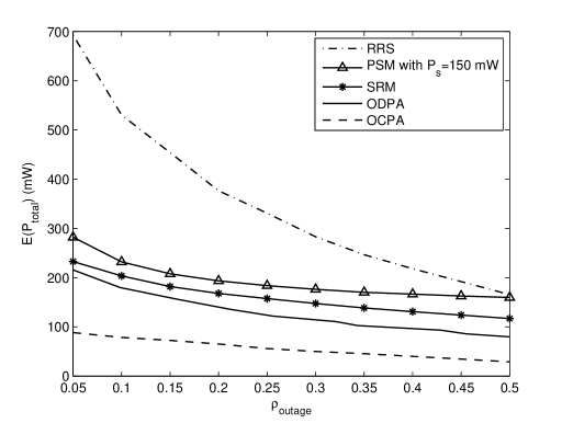
Figure 3: $E[P_{total}]$ vs $\rho_{outage}$ for different power allocation schemes.

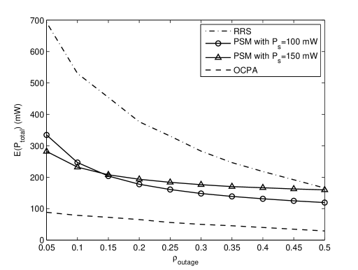
Figure 4: $E[P_{total}]$ vs $\rho_{outage}$ for the passive source model (PSM).

We also compare all of the proposed distributed power allocation schemes in Figure 3. As expected, we observe that the best performing scheme is ODPA. Passive source model (PSM) and single relay model (SRM) both have some performance loss due to the fact that, for PSM the values of the source power $P_{s}$ and the threshold $\gamma$ are fixed; for SRM only one relay node is used for forwarding transmission. However, the two special cases still outperform RRS by considering the limited available CSI for power allocation, and they simplify the optimization process of ODPA and facilitate the implementations. Thus, PSM and SRM may be preferred when computational complexity is at a premium. When $\rho_{outage}=0.05$, approximately, $80\%$, $77\%$ and $67\%$ power is saved by ODPA, SRM and PSM with respect to RRS, respectively.

Figure 4 remarks that the performance of the system with PSM depends strongly on the value of the source power (which is fixed). For low outage probability values, a high source power is favorable since it reduces the SNR contribution from the relay nodes, and hence the transmit power of the relay nodes. On the other hand, for high outage probability values, the source power becomes a lower bound for the total power. Thus, a low source power is preferred in this case.

We also investigate the effect of the direct link on the performance. Figure 5 and Figure 6 show the effect of the direct link SNR contribution on PSM and SRM, respectively. It is observed that a small amount of power savings is obtained when the direct link is considered. This amount vanishes as the quality of the direct link decreases. With this observation, when the direct link has a poor channel quality, the transmitting relay $i$ can forward the signal with power $SNR_{target}/\left|g_{i}\right|^{2}$ instead of $SNR^{\prime}_{target}/\left|g_{i}\right|^{2}$ without a significant performance loss. Employing such a strategy has the advantage that, the direct link, $h$, is not required for calculating $SNR^{\prime}_{target}$, and thus the amount of feedback from the destination is reduced.

Figure 5: Effect of the direct link SNR contribution on the passive source model (PSM) ($P_{s}=150~{}mW$).

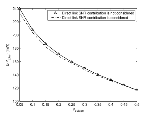
Figure 6: Effect of the direct link SNR contribution on the single relay model (SRM).

Figure 7: Comparison of the relay-assisted transmission scheme ODPA and the direct transmission scheme.

In addition, to show the power efficiency advantage of the relay-assisted transmission scheme ODPA, we compare the performances of ODPA and the direct transmission scheme where the signal is transmitted from the source to the destination via the direct link only. To show that ODPA benefits more general networks than the one we considered in Figure 2 where the direct link distance is larger than that of any source-to-relay or relay-to-destination link, we now consider that the destination’s position is randomly chosen in the area of $X\times Y=[20,100]\times[-50,50]$ for each realization, while the source and relay nodes remain in the same position as in Figure 2. In Figure 7, we plot the expected value of total power expenditure, $E[P_{total}]$, versus the target outage probability, $\rho_{outage}$, for ODPA and the direct transmission scheme. We observe that in the absence of the relays, direct transmission scheme requires a relatively high power expenditure to achieve the same outage probability as compared to ODPA. It is observed that the proposed relay-assisted transmission scheme provides significant performance gain in terms of power efficiency upon the direct transmission. This is intuitively pleasing since the relay selection and power allocation algorithms in the proposed scheme guarantee that the more power efficient way is always selected out of the relay-assisted transmission and the direct transmission for each channel realization.

VI Conclusion

In this paper, we addressed the distributed power allocation problem for parallel relay networks. Given the partial CSI available at the source and the relay nodes, we proposed a distributed relay decision mechanism and developed the optimum distributed power allocation scheme. By optimizing the relay selection strategy and power allocation, the optimum distributed power allocation strategy performs close to the optimum centralized scheme. We have also considered two simple distributed power allocation strategies, the passive source model and the single relay model. Both schemes have significantly less computational complexity requirements at the source with a modest sacrifice in performance. Our main result is that by using distributed power allocation and partial CSI, we can develop power efficient transmission schemes, reducing the amount of control traffic overhead for relay-assisted communications.

References

- [1] T. M. Cover and A. A. El Gamal. Capacity theorems for the relay channel. IEEE Transactions on Information Theory, IT-25(5):572 – 584, September 1979.
- [2] A. Sendonaris, E. Erkip, and B. Aazhang. User cooperation diversity-part I: System description. IEEE Transactions on Communications, 51(11):1927 – 1938, November 2003.
- [3] A. Sendonaris, E. Erkip, and B. Aazhang. User cooperation diversity-part II: Implementation aspects and performance analysis. IEEE Transactions on Communications, 51(11):1939 – 1948, November 2003.
- [4] J. N. Laneman, D. N. C. Tse, and G. W. Wornell. Cooperative diversity in wireless networks: Efficient protocols and outage behavior. IEEE Transactions on Information Theory, 50(12):3062 – 3080, December 2004.
- [5] J. N. Laneman and G. W. Wornell. Distributed space-time-coded protocols for exploiting cooperative diversity in wireless networks. IEEE Transactions on Information Theory, 49(10):2415 – 2425, October 2003.
- [6] A. Stefanov and E. Erkip. Cooperative coding for wireless networks. IEEE Transactions on Communications, 52(9):1470 – 1476, September 2004.
- [7] M. Janani, A. Hedayat, T. Hunter, and A. Nosratinia. Coded cooperation in wireless communications: Space-time transmission and iterative decoding. IEEE Transactions on Signal Processing, 52(2):362 – 371, February 2004.
- [8] P. Gupta and P. R. Kumar. Towards an information theory of large networks: an achievable rate region. IEEE Transactions on Information Theory, 49(8):1877 – 1894, August 2003.
- [9] G. Kramer, M. Gastpar, and P. Gupta. Cooperative strategies and capacity theorems for relay networks. IEEE Transactions on Information Theory, 51(9):3037 – 3063, September 2005.
- [10] A. Ribeiro, X. Cai, and G. B. Giannakis. Symbol error probabilities for general cooperative links. IEEE Transactions on Wireless Communications, 4(4):1264 – 1273, May 2005.
- [11] P. A. Anghel and M. Kaveh. Exact symbol error probability of a cooperative network in a Rayleigh-fading environment. IEEE Transactions on Wireless Communications, 3(5):1416 – 1421, September 2004.
- [12] A. Host-Madsen and J. Zhang. Capacity bounds and power allocation for wireless relay channels. IEEE Transactions on Information Theory, 51(6):2020 – 2040, June 2005.
- [13] D. R. Brown III. Resource allocation for cooperative transmission in wireless networks. In 38th Asilomar Conference on Signals, Systems and Computers, November 2004.
- [14] A. Reznik, S. R. Kulkarni, and S. Verdú. Degraded Gaussian multirelay channel: capacity and optimal power allocation. IEEE Transactions on Information Theory, 50(12):3037 – 3046, December 2004.
- [15] M. O. Hasna and M. -S. Alouini. Optimal power allocation for relayed transmissions over Rayleigh-fading channels. IEEE Transactions on Wireless Communications, 3(6):1999 – 2004, November 2004.
- [16] M. Dohler, A. Gkelias, and H. Aghvami. Resource allocation for FDMA-based regenerative multihop links. IEEE Transactions on Wireless Communications, 3(6):1989 – 1993, November 2004.
- [17] I. Maric and R. Yates. Forwarding strategies for Gaussian parallel-relay networks. In Conference on Information Sciences and Systems, CISS’04, March 2004.
- [18] X. Cai, Y. Yao, and G. B. Giannakis. Achievable rates in low-power relay links over fading channels. IEEE Transactions on Communications, 53(1):184 – 194, January 2005.
- [19] J. Luo, R. S. Blum, L. J. Cimini, L. J. Greenstein, and A. M. Haimovich. Link-failure probabilities for practical cooperative relay networks. In IEEE 61st Vehicular Technology Conference, VTC’05 Spring, May 2005.
- [20] Z. Lin and E. Erkip. Relay search algorithms for coded cooperative systems. In IEEE Global Telecommunications Conference 2005, Globecom’05, November 2005.
- [21] H. Zheng, Y. Zhu, C. Shen, and X. Wang. On the effectiveness of cooperative diversity in ad hoc networks: a MAC layer study. In IEEE International Conference on Acoustics, Speech, and Signal Processing, ICASSP’05, March 2005.
- [22] T. E. Hunter and A. Nosratinia. Distributed protocols for user cooperation in multi-user wireless networks. In IEEE Global Telecommunications Conference 2004, Globecom’04, December 2004.
- [23] P. Herhold, E. Zimmermann, and G. Fettweis. A simple cooperative extension to wireless relaying. In 2004 International Zurich Seminar on Communications, pages 36 – 39, 2004.
- [24] A. Bletsas, A. Khisti, D. P. Reed, and A. Lippman. A simple cooperative diversity method based on network path selection. IEEE Journal on Selected Areas of Communications, 24(3):659 – 672, March 2006.