The Trails of Superluminal Jet Components in 3C 111

Abstract

In 1996, a major radio flux-density outburst occured in the broad-line radio galaxy 3C 111. It was followed by a particularly bright plasma ejection associated with a superluminal jet component, which has shaped the parsec-scale structure of 3C 111 for almost a decade. Here, we present results from 18 epochs of Very Long Baseline Array (VLBA) observations conducted since 1995 as part of the VLBA 2 cm Survey and MOJAVE monitoring programs. This major event allows us to study a variety of processes associated with outbursts of radio-loud AGN in much greater detail than has been possible in other cases: the primary perturbation gives rise to the formation of a leading and a following component, which are interpreted as a forward and a backward-shock. Both components evolve in characteristically different ways and allow us to draw conclusions about the work flow of jet-production events; the expansion, acceleration and recollimation of the ejected jet plasma in an environment with steep pressure and density gradients are revealed; trailing components are formed in the wake of the primary perturbation possibly as a result of coupling to Kelvin-Helmholtz instability pinching modes from the interaction of the jet with the external medium. The interaction of the jet with its ambient medium is further described by the linear-polarization signature of jet components traveling along the jet and passing a region of steep pressure/density gradients.

1. Introduction

Direct evidence for the existence of bulk relativistic outflows along the jets in blazars and other radio-loud active galactic nuclei (AGN) comes from Very-Long-Baseline Interferometry (VLBI) observations. The first evidence for apparently superluminal structural changes was found from changes in the fringe visibility curves of 3C 279 and 3C 273 (Whitney et al., 1971; Cohen et al., 1971). Subsequent higher-quality VLBI observations (see, e.g., compilation by Vermeulen & Cohen, 1994, and references therein) have established the “core-jet” type milliarcsecond-scale structure of compact extragalactic jets: the core being a bright and unresolved flat-spectrum component at the end of a linear structure, and the jet being composed out of individual steep-spectrum components or “knots”. The knots frequently move away from the core with apparent velocities exceeding the speed of light. Monitoring observations of large source samples (Vermeulen & Cohen, 1994; Jorstad et al., 2001; Kellermann et al., 2004; Piner et al., 2007) have provided important statistical tools for probing relativistic beaming and the intrinsic properties of extragalactic radio jets (Cohen et al., 2007), their intrinsic brightness temperatures (Homan et al., 2006), or their Lorentz factor distribution (Kellermann et al., 2004) and luminosity function (Cara & Lister, 2007).

The relativistic-jet model (e.g., Blandford & Konigl, 1979) has become the de-facto paradigm in multiwavelength research on blazars and other AGN, but VLBI observations have demonstrated that the basic concept of ballistically-moving isolated jet knots is clearly oversimplified: jet curvature (e.g., Vermeulen & Cohen, 1994), stationary components (e.g., Jorstad et al., 2001), and non-radial and accelerated motions (e.g., Kellermann et al., 2004), are found to be common features of relativistic jets. Within individual jets, there are often characteristic velocities suggesting the presence of an underlying continuous jet flow, but the “components” themselves most likely represent patterns moving at a different speed than the underlying flow, e.g., as hydrodynamically propagating shocks (Marscher & Gear, 1985; Hughes et al., 1985).

Recent years have brought major improvements in numerical simulations of relativistic jets (see, e.g., Gómez, 2005, for a review). It is now possible to simulate three-dimensional relativistic jets (e.g., Aloy et al., 2003) and to compute the relativistic processes (e.g., Gómez et al., 1997) that transfer hydrodynamic results into observed brightness distributions (e.g., relativistic light abberation and light travel time delays). In particular, interactions between strong perturbations or shocks with the underlying jet flow and the jet-ambient medium can be simulated (Agudo et al., 2001). With these new techniques, it is now possible to compare the generation, propagation and evolution of emission features in simulated and observed relativistic jets.

The nearby (z$=$0.049) broad-line radio galaxy 3C 111 (PKS B 0415+379) shows a classical FR II morphology on kiloparsec-scales spanning more than 200^′′ with a highly collimated jet connecting the central core and the northeastern lobe in position angle 63^∘ while no counterjet is observed towards the southwestern lobe (Linfield & Perley, 1984). This asymmetry is usually explained via relativistic boosting of the jet and de-boosting of the counter-jet. 3C 111 exhibits the brightest compact radio core at cm/mm wavelengths of all FR II radio galaxies, a blazar-like spectral energy distribution (Sguera et al., 2005), and it was one of the first (and only) radio galaxies in which superluminal motion was detected (Goetz et al., 1987; Preuss, Alef, & Kellermann, 1988). Moreover, the (sub-) parsec scale jet of 3C 111 is intimately related to its high-energy emission: Marscher (2006) reports a disk-jet connection, similar to the well-established one in 3C 120 (Marscher et al., 2002), in the sense that dips in the X-ray light curve indicate accretion events which are followed by VLBI jet component ejections. Recently, R.C. Hartman & M. Kadler (in prep.) showed that the gamma-ray source 3EG J0416+3650 can be decomposed into multiple individual sources inside the EGRET full-band point-spread function, revealing a significant signal from the nominal position of 3C 111 in the higher-resolution, high-energy band above 1 GeV. This association of 3C 111 with 3EG J0416+3650, which had originally been suggested by Hartman et al. (1999) and Sguera et al. (2005), makes 3C 111 one of the very rare radio galaxies detected at gamma-ray energies and supports the view that this source may be considered a lower-luminosity version of powerful radio-loud quasars.

Here, we report the results from ten years of Very-Long-Baseline Interferometry (VLBI) observations of 3C 111 as part of the VLBA 2 cm Survey (Kellermann et al., 1998; Zensus et al., 2002; Kellermann et al., 2004; Kovalev et al., 2005) and its follow-up program MOJAVE (Lister & Homan, 2005; Homan & Lister, 2006). We investigate the parsec-scale source structure during a major flux-density outburst and during its aftermath. We find that this outburst was associated with the formation of an exceptionally bright feature in the jet of 3C 111. A variety of processes (beyond the predictions of simple ballistic motion models) are observed and discussed in view of modern relativistic-jet simulations. In Sect. 2, our observations and the data reduction are described. A detailed report of the observational results is given in Sect. 3. In Sect. 4, we discuss the various processes observed in the jet of 3C 111 as a result of the outburst and during the propagation of the new jet feature along the jet. In Sect. 5, we put these results into the context of future simulations and observations with the goal of understanding the production mechanisms of AGN jets.

2. Observations and data analysis

3C 111 has been monitored as part of the VLBA 2 cm Survey program since April 1995. The observational details are given by Kellermann et al. (1998). Following the methods described there, the data from 17 epochs of VLBA observations of 3C 111 between 1995 and 2005 (see Table 1) were phase and amplitude self calibrated and the brightness distribution was determined via hybrid mapping. An additional epoch from June 2000 was made available to us by G. Taylor. The polarization calibration was performed as described in Lister & Homan (2005). Two-dimensional Gaussian components were fitted in the $(u,v)$-domain to the fully calibrated visibility data of each epoch using the program difmap (Shepherd, 1997). The parameters of each model fit at the various epochs are given in Table 2. The models were aligned by assuming the westernmost component (namely, the “core”) to be stationary so that the position of jet components can be measured relative to it. Because of the coupling of the flux densities of nearby model components, the uncertainties in the component flux densities are larger than the formal (statistical) errors unless the given model component is far enough from its closest neighbor. Throughout this paper, errors of 15 % are assumed for the flux densities of individual model-fit components. In most cases, this should be considered a conservative estimate that accounts for absolute calibration uncertainties and formal model-fitting uncertainties (see, e.g., Homan et al., 2002). Position uncertainties were determined internally from the deviations of the data from linear motion.

3. Results

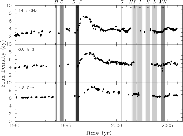
Figure 1.— University of Michigan Radio Astronomy Observatory light curves of 3C 111 at 4.8 GHz, 8 GHz, and 14.5 GHz. The shaded areas indicate the ejection epochs of the individually labeled jet components as discussed in Sect. 3.2. The lightest shading corresponds to minor ejections of the relatively weak components I,J,K,L with flux densities $S$ below $0.2$ Jy, medium shading corresponds to components B,C,G,H,M,N with $0.2{\rm Jy}<S<0.6{\rm Jy}$ and the darkest shading to components E and F with $S>0.6{\rm Jy}$.

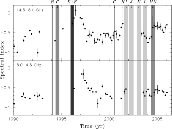
Figure 2.— Spectral-index curves of 3C 111 between 14.5 GHz and 8 GHz (top), and 8 GHz and 4.8 GHz (bottom) from the UMRAO monitoring program. The shaded areas are the same as in Fig. 1.

3.1. The 1996 Radio Outburst of 3C 111

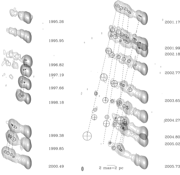
Figure 3.— Naturally weighted images of the parsec-scale jet of 3C 111 from the 2 cm VLBA monitoring. A common restoring beam of $(0.5\times 1.0)$ mas at P.A. $0^{\circ}$ was used. The total recovered flux density in each image, the rms noise, and the lowest contours for each image are given in Table 1. Contours increase logarithmically by a factor of $2$. Only components E, G, H and their corresponding trailing components are indicated by circles enclosing a cross.

A strong flux density outburst of 3C 111 occurred in 1996, which was first visible in the mm band and some months later at lower radio frequencies. This outburst was first detected at 90 GHz with the IRAM interferometer at Plateau de Bure in January 1996 with flux densities greater than $10$ Jy (Alef et al., 1998), at 37 GHz in March 1996, and at 22 GHz in August 1996 with the Metsähovi radio observatory (Teräsranta et al., 2004). Figure 1 shows the single-dish radio light curves of 3C 111 at 4.8 GHz, 8 GHz, and 14.5 GHz obtained from the UMRAO radio-flux-density monitoring program (Aller, Aller, & Hughes, 2003). These data show that from early 1996 on, the radio-flux density of 3C 111 was rising at 14.5 GHz, reaching its maximum in late 1996. At the two lower frequencies, the flux-density maximum was reached at subsequent later times, in mid 1997 at 8 GHz and in late 1997 at 4.8 GHz. The profile of the outburst in the flux-density vs. time domain shows a narrow, high-amplitude peak between early 1996 and late 1997, which is almost symmetric. After late 1997, a slower-decreasing component dominates the light curves, most clearly visible at 14.5 GHz.

Figure 1 shows that the flare propagated through the spectrum as qualitatively expected by standard jet theory (e.g., Marscher & Gear, 1985): high-frequency radio emission comes from the most compact regions of the jet, the emission peak shifts to lower frequencies as a newly ejected jet component travels down the jet and becomes optically thin. The peak flux density shifted with frequency at about $10$ GHz yr^-1.

The evolution of the spectral index, $\alpha$ ($S\sim\nu^{\alpha}$), for (14.5/8.0) GHz and (8.0/4.8) GHz is shown in Fig. 2. Before 1996, the sampling was too sparse to derive the change of the spectral index in the (14.5/8.0) GHz band. Between, 8.0 GHz and 4.8 GHz, the spectral index was approximately $-0.7$ during the pre-1996 period. The radio flux-density outburst in 1996 corresponded to a subsequent flattening of the spectrum with a maximum spectral index, $\alpha\sim 0$, in the (14.5/8.0) GHz band reached in mid 1996. In the post-outburst period between 1998 and 2004, $\alpha$ was typically in the range $-0.5$ to $-0.7$ between 14.5 GHz and 8.0 GHz and slightly steeper ($-0.7$ to $-0.9$) in the (8.0/4.8) GHz band. The overall steeper spectral index at lower frequencies can be understood as the contribution of optically thin large-scale emission from the radio lobes of 3C 111 to these single-dish light curves.

3.2. VLBA Monitoring Results

Figure 3 shows the variable parsec-scale structure of 3C 111 at 18 different epochs of VLBA observations between 1995.26 and 2005.73. The variable source structure can be described by a classical one-sided core-jet morphology in the first two epochs with typical velocities of the outward moving jet components of about $1.4$ to $1.7$ mas yr^-1 corresponding to about $5$ $c$. In 1996.82 a new jet component, even brighter than the core, dominated the source structure. By 1997.19, this new component was even brighter ($\sim 3.4$ Jy) and in the following epochs it traveled along the jet while it became gradually more stretched out along the jet-ridge line.

Model Fitting:

In Fig. 4, the radial distance of the various model fit components from the core is shown as a function of time. The component identification was based on a comparison of the positions and flux densities, and a linear regression of the distances from the core as a function of time was used to determine the kinematics. The derived component velocities are tabulated in Table 3. The early outer jet components (A, B, C, D) of the 1995.26 epoch can be traced over two to four epochs before their flux densities fall below the detection threshold (compare Fig. 5). In late 1996 and early 1997, the source structure was dominated by the emission of the core and the newly formed jet components E and F, with E being the leading component. The two components traveled outwards with a mean apparent velocity of $(1.00\pm 0.02)$ mas yr^-1 and $(0.64\pm 0.07)$ mas yr^-1, respectively. Before mid 1997, component F was substantially brighter than component E but after that, its flux density dropped steeply. F was not detected at any epoch later than 1998.18, while E was still about $800$ mJy at that time. The light curves of E and F reproduce qualitatively the two-component shape of the flux-density outburst in Fig. 1 with component F being responsible for the narrower and higher-amplitude peak between early 1996 and late 1997 and component E dominating the slower-decreasing tail of the outburst after late 1997 (compare Fig. 5 and discussion below). In the following epochs, E split into four distinct components (E 1, E 2, E 3, E 4) at distances of 3.5 mas to 4.5 mas from the core. E 2, E 3, and E 4 all moved at subsequently slower speeds than E 1, resulting in an elongated morphological structure of the associated emission complex.

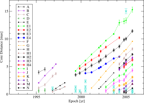
Figure 4.— Core separation of model-fit components vs. time. Crosses represent components which could not be cross identified over the epochs. Position uncertainties have been estimated from the internal deviations of the data from linear motions for each component. The uncertainties for the position of E 1 have been determined separately for the pre-2004 and post-2004 epochs because of the partial resolution of this component after 2004. Uncertainties for components with less than three epochs were estimated from other components at similar positions in the jet and with similar flux densities.

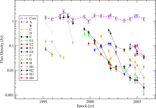
Figure 5.— Flux-density evolution of the core and the jet components with time. For clarity, only components ejected before 2001.50 are shown. The flux densities of E 1, E 2, E 3, and E 4 were added for the post-1999 epochs and a flux-density weighted effective position was calculated to display the flux-density evolution of the blended feature that would be visible at lower resolution. Note that components E 4 and G are blended in epoch 2004.27 and that the flux density of E 4 may be overestimated for this epoch.

In later epochs, new components have been ejected from the core into the jet. The two strongest components (G,H) can be traced through the following eight and nine monitoring epochs, respectively. Component H split into three individual components in 2004.27 and a fourth associated component was seen from 2004.80 on. In the following, we refer to the components E 1, and H 1 as the “leading components” and to E 2, E 3, E 4, H 2, H 3, and H 4 as the “trailing components” of E and H, respectively.

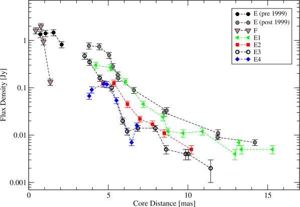
Figure 6.— Flux-density evolution of component E and its trailing components vs. the distance traveled from the core. Note that component E 4 is blended with component G in epoch 2004.27 and that its flux density may be overestimated for this epoch.

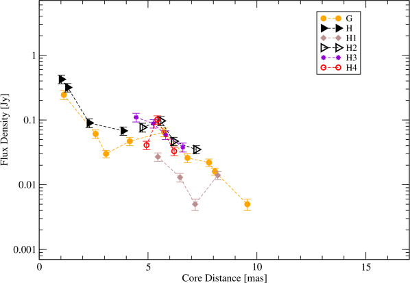
Figure 7.— Flux-density evolution of component G and H and its trailing components vs. distance traveled from the core.

For the pc-scale jet of 3C 111, the ejection epochs of the individual jet components can be determined from the linear regression by back-extrapolating the component trajectories to the core. In Fig. 1, these ejection epochs and the associated uncertainties are indicated as shaded areas. It is apparent that the ejection of the components E and F coincides with the onset of the major flux-density outburst in 1996 described above. The following major component ejections (G, H, and the combined M/N event) all have direct counterparts in local maxima of the radio light curve, especially at 14.5 GHz. Figure 2 shows that all these ejection epochs coincided with local maxima of the spectral index in the 14.5/8.0 GHz band. Between 2002 and 2004, a number of minor component ejections took place but the regression-fit quality (due to the neareby components, the low flux densities and the small time baseline) only moderatly constrains the ejection epochs. In addition, the time sampling of UMRAO observations in this time range is relatively poor, in particular from mid 2001 to mid 2003.

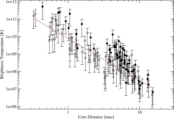
Figure 8.— Brightness temperatures of model-fit components as a function of their distance to the core. The brightness temperatures of components belonging to the E–, F– and H–components are indicated by filled black circles. The solid line represents a least-squares fit to all but the E–, F– and H–components. The slope of the regression curve is $-2.4\pm 0.2$.

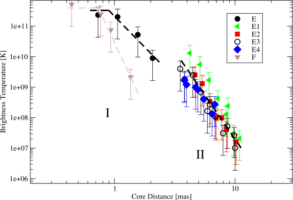
Figure 9.— Brightness temperatures of component E, its leading and trailing components, and component F as a function of their distance to the core. The two regimes of brightness-temperature gradient discussed in the text are indicated with dashed lines.

Flux Density Evolution:

Figure 5 shows the brightness evolution of the core and the jet components that have been ejected prior to 2001.5. Apparently, the trailing components E 4 and H 4 appeared first in a rising state, i.e., they first increased in flux density before they became fainter in later epochs. Component F showed an extraordinary steep decrease in brightness in 1997–1998. In Fig. 6 and Fig. 7, the flux-density evolution of the components E, G, and H and the associated leading and trailing components are shown with distance traveled from the core, respectively. The ejecta first rose in flux density within the inner 1 mas from the core, then they showed a decline about almost three orders of magnitude in the following decade, exhibiting a plateau or broad local maximum in 1998–2000 at a distance from 2–4 mas from the core. Component H and its leading and trailing components exhibited a similar behavior although on about an order of magnitude lower flux-density levels and at slightly further downstream, 4–6 mas from the core. Component G, in spite of the fact that it does not appear to have split into leading and trailing components like E and H, did exhibit a pronounced flux density maximum after 2002, as well, about 6 mas from the core.

The T_b gradient along the jet:

Following Kadler et al. (2004); Kadler (2005), the power-law index $s$, which describes the brightness temperature gradient via $T_{\rm b}\propto r^{s}$, can be parametrized as

$$s\,=\,l\,+\,n\,+\,b\,(1\,-\,\alpha)$$ (1)

where $l$, $n$ and $b$ are the power law indices that describe the gradients of jet diameter $d\propto r^{l}$, particle density $n_{e}\propto r^{n}$, and magnetic field $B\propto r^{b}$ with distance $r$ from the core, respectively. Therefore, measuring the brightness temperature gradient provides a method to constrain the critical physical properties along the jet and abrupt changes in the $T_{\rm b}$-gradient can highlight regions in the jet where the density, magnetic field, or jet diameter change rapidly.

Figure 8 shows the brightness temperatures of all jet components in the parsec-scale jet of 3C 111 at 2 cm wavelength between 1995 and 2005 as a function of their core distance. In general, the brightness temperature of all components decreased as the components traveled outwards but an approximation with a simple power law does not yield a good fit to the full data set ($\chi_{\rm red}^{2}=1.8$, 115 degrees of freedom [d.o.f.]). Visual inspection of Fig. 8 shows that this is due to the E–, F– and H– components and their leading and trailing components, respectively. This behavior is different than expected for a straight and stable jet geometry in which the power-law dependences of the particle density, the magnetic field strength and the jet diameter on the core distance predicts that the brightness temperature along the jet can be described with a well-defined power-law index $s$. Most extragalactic parsec-scale jets which do not show pronounced curvature, show a power-law decrease with increasing distance from the core and power-law indices typically around $-2.5$ (Kadler, 2005). In fact, excluding the E–, F– and H–components from the fit yields a statistically better result ($\chi_{\rm red}^{2}=1.3$, 52 d.o.f.) and a gradient of $-2.4\pm 0.2$. In Sect. 4.1 and Sect. 4.5, we discuss possible physical reasons for the different behavior and nature of these components. The measured relation between component sizes and distance along the jet is affected by a large degree of scatter and does not provide independent information from the flux density and brightness temperature plots described above. Therefore we do not show plots of component size versus jet distance.

The brightness-temperature gradient of component E was first flat or inverted immediately after the creation of this new component within approximately 1 mas from the core and then reached steep values of $-2.5$ to $-2.8$ (regime I; compare Fig. 9) through 1997 when the component traveled from 1 mas to 2 mas. Between 2 mas and 4 mas, the determination of the brightness-temperature gradient requires an identification of component E with either component E 1 or E 3 (see below). Independently of this identification, the brightness-temperature gradient eventually changed to very steep values ($s<-5$) beyond 5 mas from the core (regime II). Component F began its very rapid decline in brightness temperature at a very small distance from the core ($<0.7$ mas) with an extremely steep $T_{\rm b}$-gradient ($s<-8$).

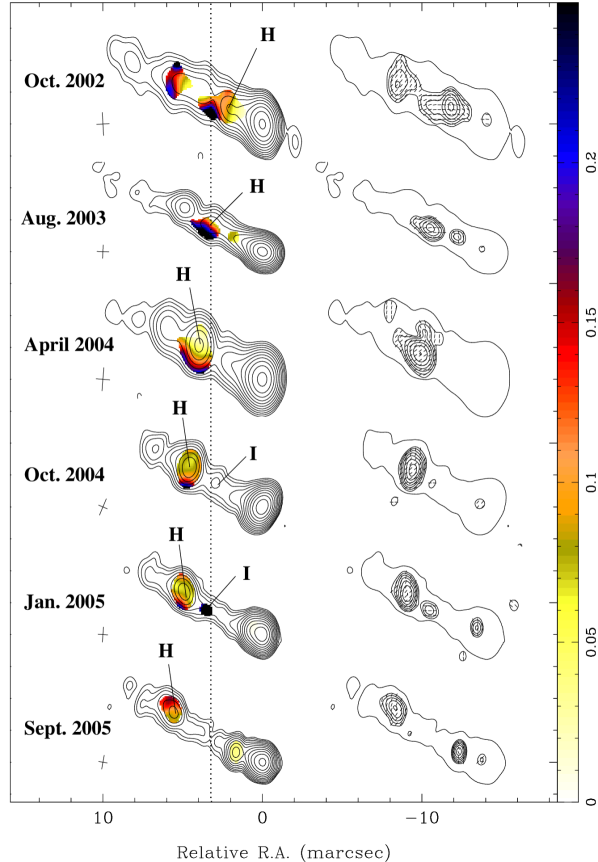
Figure 10.— Naturally weighted images of the linear-polarization structure of 3C 111 between 2002 and 2005. The restoring-beam dimensions and orientations for each epoch are indicated by a cross to the left of each Stokes-I image. Stokes I contours start at 1 mJy/beam and increase by factors of $2$. Fractional polarization is over-plotted on the Stokes-I contours in color. To the right of the Stokes-I images are the polarization intensity contours starting at 1 mJy/beam and increasing by factors $\sqrt{2}$. The polarization contours are over-plotted with tick-marks representing the electric vector position angle. A single Stokes-I 1 mJy contour surrounds the polarization image to show registration. The dotted line marks the distance of 3.3 mas from the core where the most pronounced changes of the polarization properties take place (see text).

Linear Polarization:

From 1995 to 2002, 2 cm-Survey observations were done in left circular polarization only, so no linear-polarization information can be derived from these data. MOJAVE observations (from 2002 on) are done in full-polarimetric mode. Figure 10 shows our polarization data through September 2005.

In October of 2002, component H was about 2.5 mas from the base of the jet and showed a fractional polarization of 5% to 10% increasing towards the downstream side of the component. The electric vector position angle (EVPA) displayed by the component was approximately aligned with the jet. In this epoch, the jet material just downstream of component H at $\sim 3.3$ mas from the base of the jet was more highly polarized, exceeding 20% fractional polarization on the jet’s southern side, and the EVPA of the polarization turned to be about 45^∘ to the main jet direction.

By August of 2003, component H had entered a region approximately $3.3$ mas from the core and its observed polarization was now similar to the emission in this same region observed in the previous epoch. The observed fractional polarization of H now climbed sharply to values in excess of 20% toward the jet’s southern side while there was no detectable polarization from the northern side of H. The observed EVPA of H had rotated further to be approximately 60^∘ to the main jet direction. However, the EVPA on the southern-most side of H was approximately perpendicular to the jet.

After component H passed through this region (epochs April 2004 through September 2005), it split into a number of subcomponents as described earlier, and its polarization gradually became more uniform. Consistent fractional polarization of 5% to 10% was approached with the electric vectors approximately perpendicular to the local jet direction.

The much weaker component, I, developed polarization very similar to H as it passed through the same region, about 3.3 mas from the core, with fractional polarization exceeding 20% toward the southern side of the jet with an EVPA at approximately 45^∘ to the main jet axis. This is also the same region of the jet in which component E had broken up into a number of sub-components. In future epochs, we will have the opportunity to follow component K as it passes through this same region.

4. Discussion

In this section, we discuss the aftermath of the major outburst in 3C 111 in 1996 and the following component ejections through 2005. We organize the subsections of our discussion according to the downstream distance from the VLBI core where we observe the effect of interest.

4.1. Within $1$ pc: Forward and Reverse Structures

Numerical simulations (Aloy et al. 2003) show that an abrupt perturbation of the fluid density at the jet injection point during a short time propagates downstream, evolves spreading asymmetrically along the jet and finally splits into two distinct regions. Both of these two regions have enhanced energy density with respect to the underlying jet, and they emit synchrotron radiation. The leading (forward shock) and the following region (reverse shock) have higher and lower Lorentz factors, respectively, than the underlying jet. Thus, they should separate with time as they propagate downstream in the jet.

Component F matches the description of a backward moving wave associated with the major injection into the jet of 3C 111 after the flux-density outburst of 1996. It follows the trail of component E but at a lower speed. If component F is identified with a reverse shock and component E with a forward shock, it is possible then to compute the size of the shocked region (Perucho et al., 2007). In 1996.82 and 1997.19, E and F were both very bright and separated by only $\sim 0.3$ pc in projected distance. During these two epochs, F was 300 mJy to 500 mJy brighter than the leading component E. Following Aloy et al. (2003), a backward shock can be brighter than a forward shock if the latter is beamed in a cone smaller than the viewing angle due to its larger speed. We have examined the Doppler factors of components E and F for the range of possible viewing angles (see Appendix A) and the measured velocities and conclude that this alone cannot explain the brightness difference between component E and F because the difference in apparent speed is not large enough. Jorstad et al. (2005) point out that backward shocks can be brighter than forward shocks as long as the disturbance is prolonged and there is a continuous supply of particles entering from the underlying jet through the shock region. Within half a year, between 1997.19 and 1997.66, F lost about half of its brightness. This extraordinarily fast dimming of the backward shock can be caused by the lack of input of particles from behind, i.e., a lower plasma ejection rate after the primary injection possibly due to a depletion of the inner accretion disk (Marscher et al., 2002; Marscher, 2006) which feeds the plasma injection.

Component F can also be interpreted as a rarefaction propagating backwards in the reference frame of the ejected blob of gas. A rarefaction is produced when the blob is overpressured with respect to the jet, as this overpressure causes the front to accelerate in the jet, thus leaving a rarefied region between the head of the blob (forward shock) and its rear part, which is still slower (it moves with the injection velocity). In this case, the emission in component F could be associated to the denser and overpressured gas in the blob which has still not been rarefied. This gas would cease to emit as soon as it reaches the rarefied region, which may also explain the sudden decrease in brightness of this component. An extended discussion on the nature of component F and the evolution of its brightness will be given in Perucho et al. (2007).

4.2. Between $2$ pc and $4$ pc: Expansion and Acceleration

It is not a-priori clear with which post-split-up component the original feature E should be identified after 1999. A natural identification would be the leading component E1 but that requires an acceleration of this component (see Fig. 4) from $\beta_{\rm app,E}=3.26\pm 0.07$ to $\beta_{\rm app,E1}=5.5\pm 0.1$ between 1998.18 and 1999.38. This may be interpreted in terms of an expansion of the jet in a rarefied medium. Taking an angle to the line of sight of $19^{\circ}$ (see Appendix A), the component would be accelerated from $\beta=0.956$ ($\gamma\sim 3.4$) to $\beta=0.995$ ($\gamma\sim 10.3$). The increase of velocity is less at smaller viewing angles.

An alternative model for the acceleration and brightening of component E would be a change of the jet inclination to the line of sight from about 24^∘ to about 11^∘ at this location in the jet as observed in the case of the quasar 3C 279 (Homan et al., 2003). However, we see no significant change in jet position angle in the sky which would be expected to accompany such a large change in jet direction. Moreover, subsequent components, particularly G, do not show the same kind of large acceleration in this region.

Direct identification of component E with component E1 is not straightforward in the frame of expansion, as component E1 in epoch 1999.38 was smaller than component E in 1998.18 (see Table 2). However, component E3 in epoch 1999.38 is larger than component E in 1998.18. We can interpret this as component E including components E1 and E3 (and maybe E4). These components would be indistinguishable in our observations before 1999.38. In fact, Jorstad et al. (2005) monitored 3C 111 between 1998 and 2001 with the VLBA at 43GHz. They find an emission complex, that can be identified with our component E, that gradually stretches out as it travels from $\sim$ 2 mas from the core in 1998 to roughly between $5$ mas and $8$ mas from the core in 2001. Their leading component C1 can be identified with our component E1, their component c2 with E2 and their c1 with E3. At their higher angular resolution, Jorstad et al. can separate components C 1 and c 1 already in early 1998. In agreement with our analysis at 15 GHz, they detect c2 (E2) about a year after they detect c1 (E3). They do not detect a component corresponding to E4 but this may be an effect of partially resolving out the jet structure at their higher observing frequency, particularly in later epochs. It is further interesting to note that the observed speeds at both frequencies agree well. For E1(C1), $\mu_{\rm app,2\,cm}=1.69\pm 0.04$ mas yr^-1 at 15 GHz and $\mu_{\rm app,7\,mm}=1.77\pm 0.06$ mas yr^-1 at 43 GHz; for E2(c2), $\mu_{\rm app,2\,cm}=1.29\pm 0.06$ mas yr^-1 at 15 GHz and $\mu_{\rm app,7\,mm}=1.23\pm 0.04$ mas yr^-1 at 43 GHz; and for E3(c1), $\mu_{\rm app,2\,cm}=1.22\pm 0.05$ mas yr^-1 at 15 GHz and $\mu_{\rm app,7\,mm}=1.07\pm 0.02$ mas yr^-1 at 43 GHz. The discrepancy in the speeds measured for E3 and c1 seems to be due to a slight acceleration of E3 after 2002. A fit to the 15 GHz data of E3 between 1999 and 2002 alone yields a slower speed of $\sim$ 1.0 mas yr^-1 similar to the speed of c1 in the same time period at 43 GHz. In their work, Jorstad et al. do not report acceleration of components from 2 mas to 4 mas. However, this is likely due to the fact that their observations started in early 1998, thus missing the first observations of component E presented in this paper, when its speed has been measured to be smaller.

4.3. Between $2$ pc and $6$ pc: Recollimation of the Jet

Inspection of Fig. 9 shows that the back-extrapolation of the brightness temperature of component E from regime II to regime I is at least two orders of magnitude too high if this extrapolation is based on the gradient given by E1. The low brightness temperature of component E in regime I cannot be explained by opacity effects because the radio-light curve in Fig. 1 shows that the source was optically thin from 1997 on. Moreover, if we identify component E with E1, it is Doppler-deboosted from epoch 1998.18 to 1999.38 due to the acceleration and a relatively large viewing angle; thus, we are not able to explain the increase in brightness temperature in terms of Doppler boosting. However, compact sub-components may have larger brightness temperatures, so that the $T_{\rm b}$ values plotted in Fig. 9 for E in regime I inward of about $3$ mas may represent lower limits for compact components already embedded in the unresolved structure.

Not only E/E1 but also components G and H show an increase in total flux density several milliarcseconds downstream. Compared to E/E1, these somewhat weaker components exhibit their flux-density maxima at somewhat larger distances from the core (compare Fig. 6 and Fig. 7). This can be explained if the gas in the components travels through a mild standing shock in a recollimation region. This effect has been observed in numerical simulations of parsec (Gómez et al., 1997) and kiloparsec scale jets (Perucho & Martí, 2007). The material in the components is expected to be overpressured with respect to its environment, thus expanding into it. After the initial expansion, the components become underpressured with respect to the underlying flow. The resulting recollimation leads to the formation of a shock, whose strength depends on the initial degree of overpressure of the material in the component. This process explains the increase in flux density and brightness temperature as due to compression of the gas in the recollimation. In Figs. 6 and 7, we see that the flux density of component E increases closer to the core than for component G and H, which is consistent with the former being slower than the latter, thus recollimating earlier (see Perucho & Martí, 2007). It also explains why we see a significant acceleration only in the faster expanding, brighter component E/E1.

Finally, after this mild recollimation, the fluid becomes overpressured with respect to its environment, thus further expanding and accelerating downstream.

4.4. Near $3$ pc: The Role of the External Medium

The polarization behavior of components H and I can be understood in terms of an interaction between the jet and the external medium at a distance of  3.3 mas ($=3.3$ pc) in the jet. Assuming no Faraday rotation, the EVPA of component H within approximately 3.3 mas from the core indicates a transverse magnetic field order as might be expected for a transverse shock propagating down the jet. The change in the fractional polarization, its north-south gradient, and the rotation of the EVPA suggest that a contact surface persists at the southern boundary of the jet beam at a distance of approximately 3.3 mas downstream the jet core. If the bulk jet material flows faster than the flow at the southern boundary, the magnetic field is stretched through shear. Our overall picture then is of an originally transverse shock interacting with the jet on the southern side of the jet at   3.3 mas from the core. The interaction changes the component’s magnetic field through some combination of oblique shock and differential flow resulting in a magnetic field approximately parallel to the jet axis in the later epochs. No strong shock is needed at this location in the jet but this region may be identified with the recollimation region (see Sect. 4.3) at about the same position in the jet). In this picture, the jet-medium interaction may form an effective nozzle which accelerates the jet on one edge relative to the other.

An alternative explanation for the observed polarization structure and dynamics of 3C 111 can be found by considering an inhomogeneous external Faraday screen. Such a screen could produce the observed differential rotation of the EVPA while a component travels through a given region along the jet. Zavala & Taylor (2002) observed 3C 111 with the VLBA and produced a Faraday rotation-measure map between 8 GHz and 15 GHz. They find strong Faraday rotation, $\sim 730$ rad m^-2, at the same distance from the core (3.3 mas) where our observations show the swing of the EVPA of the component H and steeply decreasing Faraday rotation further downstream. However, we note that $730$ rad m^-2 translates to 17^∘ of rotation at 15 GHz which alone is not enough to explain the change in EVPA that we observe while component H travels through this region. On the other hand, the steep decrease of the Faraday rotation measured up- and downstream of this region by Zavala & Taylor (2002) again agrees with a change of the external gas density at this point, which in turn may be identified with the pressure gradient responsible for the component expansion and accelleration.

A combination of inhomogeneous Faraday rotation and an interaction between the jet plasma and its ambient medium appears most likely to explain our observations of the varying linear polarization structure; however, both explanations point to the role of the external medium, either through a discrete interaction or a rapid decrease in external gas pressure, in shaping the jet flow downstream of this location.

4.5. Between $3$ pc and $5$ pc: Formation of Trailing Components

The components E2, E3, and E4 can be interpreted as trailing components forming in the wake of the leading E1 which is identical with the original component E. This scenario is attractive because the basic concept of trailing components as introduced by Agudo et al. (2001) predicts the formation of trailing features in the wake of the initial perturbation in the jet flow. Such a behaviour has first been found both associated with bright sub- and superluminal jet components in Centaurus A and 3C 120 (Tingay, Preston, & Jauncey, 2001; Gómez et al., 2001). Jorstad et al. (2005) report trailing components in four additional sources (3C 273, 3C 345, CTA 102 and 3C 454.3) and in 3C 111 (see below).

The interaction of the external medium with a strong shock pinches the surface of the jet, leading to the production of pinch-body mode Kelvin- Helmholtz instabilities: the trailing features. Hence, a single strong superluminal shock ejection from the jet nozzle may lead to the production of a multiple set of emission features through this mechanism. The trailing features have a characteristic set of properties, which make them recognizable with high resolution VLBI: they form in the wake of strong components instead of being ejected from the core of VLBI jets, they are related to oblique shocks, they are always slower than the leading feature, and (if the underlying jet has a certain opening angle) they should be generated with a wide range of apparent speeds (from almost stationary near the core to superluminal further downstream). Moreover, Agudo et al. (2001) showed that the separation between the trailing components increases downstream due to their motion down a pressure gradient.

All this is in agreement with what we observe in the trailing components of E 1 and with our interpretation of an expansion of the jet in a density decreasing ambient medium. For the time range covered by their observations (1998.23 to 2001.28), Jorstad et al. (2005) also identified the trailing phenomenology in this source.

The north-south gradients detected in the linear-polarization emission in the region where the trailing features are formed, is in agreement with an oblique shock structure. The steep brightness-temperature gradients of the trailing components indicate that the particle and magnetic field density associated with these components evolve in a different way compared to the “normal” jet flow. These shocked regions may be more overpressured with respect to their environment, making them expand rapidly. This fast expansion implies a larger positive value of $l$, which, however, is compensated by an even larger (negative) value of $n$ and $b(1-\alpha)$ in equation 1, resulting in a very steep brightness temperature gradient (regime II).

Pinching modes of the Kelvin-Helmholtz instability were shown to couple to the trailing components observed in the simulations in Agudo et al. (2001). In the case of components E2-E4, the distance between them ranges from 0.7-0.8 mas at the first epochs in which they are observed, to almost 2.0 mas in the latest epochs. Taking into account that: a) their FWHM is of the same order (see Table 2); b) that these wavelengths have to be corrected for geometrical and relativistic effects, resulting in a maximum intrinsic wavelength of $\sim 0.7\,\rm{mas}$, and c) that the size of the components can be of the order or smaller than the jet radius (Perucho & Lobanov 2007), this implies coupling of the pinching to wavelengths of the order or smaller than the jet radius. Perucho et al. (2007) have shown that resonant Kelvin-Helmholtz instabilities associated to high-order body modes appear in sheared jets at these wavelengths. These modes have larger growth rates than low-order body modes or surface modes, and their growth brings the jet to a final quasi-steady state in which it remains well-collimated and generates a hot shear-layer which shields the core of the jet from the ambient medium. Interestingly, the jet in 3C 111 is known to be well-collimated up to kiloparsec scales. Further research in this direction is needed in order to check the influence of the resonant modes in the long term evolution of this jet.

A by-product of the interpretation of these components as Kelvin-Helmholtz instabilities is the fact that it allows us to put constraints to the velocity of the jet. We can regard the wave speed as the minimum speed of the jet flow, as KH modes have an upper limit in their wave speeds that is precisely the velocity of the flow in which they propagate (Perucho et al., 2006). The upper limit is given by the speed of E1, interpreted as a shock wave, that has to be thus faster than the underlying flow. In this picture, we would have the structure E1 moving with Lorentz factor $\gamma\sim 8.3$ through a jet with Lorentz factor $8.3>\gamma_{j}\geq 4.6$ in the accelerated region (post 1999.38), where the lower limit is given by the Lorentz factor of component E2, the fastest of the three trailing components identified here.

5. Summary and Conclusions

In this paper, we have investigated the parsec-scale jet kinematics and the interaction of the jet with its ambient medium in the broad-line radio galaxy 3C 111. Our analysis has demonstrated that a variety of processes influence the jet dynamics in this source: a plasma injection into the jet beam associated with a major flux-density outburst leads to the formation of multiple shocks that travel at different speeds downstream and interact with each other and with the ambient medium. The primary perturbation causes the formation of a forward and a backward shock (or rarefaction). The latter fades away so fast that is likely to remain undetected in minor ejections. A separate work by Perucho et al. (2007) focuses on the nature and characteristics of these initial components. Several parsecs downstream, the jet plasma enters a region of rapidly decreasing external pressure, expands into the jet ambient medium and accelerates. In the following, the plasma gets recollimated and trailing features are formed in the wake of the leading component.

A particularly interesting aspect of the source 3C 111 in the light of this and other recent works is that it is one of the very rare non-blazar gamma-ray bright AGN. Besides Centaurus A (Sreekumar et al., 1999) and the possible identification of NGC 6251 with the EGRET source 3EG J1621+8203 (Mukherjee et al., 2002), 3C 111 is the only AGN whose jet-system is inclined at a relatively large angle to the line of sight and that has a reliable EGRET identification: Sguera et al. (2005) reconsidered the possible identification of the EGRET source 3EG J0416+3650 with 3C 111, which was first suggested by Hartman et al. (1999) but considered unlikely because of the poor positional coincidence. Very recently, R. C. Hartman & M. Kadler (in prep.) found that 3EG J0416+3650 is composed out of at least two distinct components. One of them is the dominant source above 1 GeV and is in excellent positional agreement with the location of 3C 111. Compared to blazars, the large inclination angle and the relatively small distance of 3C 111 allow us to resolve structures along the jet that are as small as parsecs in deprojection and which would be heavily blended with adjacent features in blazar jets. As demonstrated in this paper, VLBA observations of 3C 111 probe a variety of physically different regions in a relativistic extragalactic jet such as a compact core, superluminal jet components, recollimation shocks and regions of interaction between the jet and its surrounding medium, which are all possible sites of gamma-ray production. From early 2008 on, the gamma-ray satellite GLAST (Lott et al., 2007) is going to monitor the sky. If detected by GLAST, 3C 111 may become a key source in the quest for an understanding of the origin of gamma-rays from extragalactic jets. In addition, the combination of GLAST and VLBA data with spectral data at intermediate wavelengths (optical, IR, X-ray) may allow a better determination of jet parameters and relativistic beaming effects than in most blazars because of the higher linear resolution offered by this nearby and only weakly projected jet system.

Our observations of 3C 111 are qualitatively in remarkable agreement with numerical relativistic hydrodynamic structural and emission simulations of jets such as the ones presented by Agudo et al. (2001) and Aloy et al. (2003). Further progress is being made in the transition from two-dimensional to three-dimensional simulations of relativistic jets and in the development of new methods considering magnetic fields (Leismann et al., 2005; Mizuno et al., 2007; Roca-Sogorb et al., 2008, e.g.,), the equation of state for relativistic gases (Perucho & Martí, 2007), and radiative processes (e.g., Mimica et al., 2004, 2007, and Mimica et al. in preparation). But so far neither observational data nor simulations have reached an adequate level of detail and completeness in order to allow us a quantitative direct comparison of numerical models and observed relativistic jet structure and evolution. In particular, it is not feasible today to fit iteratively the parameters of relativistic magneto-hydro-dynamical (RMHD) jet simulations to match the brightness distribution observed for any individual source. The main reasons for this are a) the immense computational power required to conduct a realistic (i.e., sufficiently detailed) modern 3D jet simulation and b) the highly non-linear nature of RMHD plasmas and their evolution. Simulation results depend critically on the starting conditions like the exact velocity, composition, and transversal structure of the flow, the structure and strength of the magnetic field and the jet environment. Future development of computational power will allow us to use larger resolutions to decrease the numerical viscosities, and to implement nonlinear and microphysics processes into simulations. VLBA observations are capable of putting hard quantitative constraints on the input parameters for RMHD jet simulations if they are densely sampled over several years. Polarimetric observations at multiple radio frequencies may allow the effects of jet-intrinsic magnetic-field variations and external Faraday-screen inhomogenities or temporal variations to be disentangled. Such data at 15 GHz are on the way, e.g., as part of the next phase of the MOJAVE program, in which rapidly evolving sources like 3C 111 are being observed every two months.

Appendix A The Jet Inclination Angle

The 1996 radio outburst of 3C 111 puts strong constraints on the angle to the line of sight for this source, if one assumes that a similarly bright component as E has been ejected in the counterjet, as well. Due to differential Doppler boosting, the flux density ratio between the jet- and counter-jet emission is

$$\frac{S_{\rm J}}{S_{\rm CJ}}=\left(\frac{1+\beta\cos{\theta}}{1-\beta\cos{\theta}}\right)^{2-\alpha}\quad.$$ (A1)

Thus, for a given jet to counter-jet ratio $x=\frac{S_{\rm J}}{S_{\rm CJ}}$

$$\beta\cos{\theta}=\frac{x-1}{x+1}\quad.$$ (A2)

With $\alpha=0.3$, $S_{\rm J}=3.4$ Jy (components E and F in 1997.19), $S_{\rm CJ}<10$ mJy and $\beta<1$, $\theta<21^{\circ}$. For a realistic jet speed of, e.g., $\beta=0.956$ ($\gamma=3.4$), the angle to the line of sight is: $\theta=19^{\circ}$. An estimate close to this value can be derived from the variability Doppler factor measured by Lähteenmäki & Valtaoja (1999) and the apparent superluminal jet speed. As outlined in detail in Cohen et al. (2007), this leads to a value of $\theta\sim 15^{\circ}$.

It is important to note that this calculation implicitly assumes symmetry between the jet and counter-jet, which in projection does not have to be the case if the counter-jet is covered by an obscuring torus as it is well-established for systems at larger inclination angles (e.g., NGC 1052: see Kadler et al., 2004). Indeed, Faraday rotation measurements towards the 3C 111 pc-scale jet (Zavala & Taylor 2002; see also Sect. 4.4) and X-ray spectral observations (Lewis et al. 2005) suggest substantial amounts of obscuring material. Free-free absorption could also substantially lower the counter-jet radio emission and allow for larger jet angles to the line of sight.

An independent lower limit on the inclination angle of $\theta>21^{\circ}$ was given by Lewis et al. (2005) assuming that the deprojected size of the largescale 3C 111 double-lobe structure is smaller than $500h^{-1}$ kpc. This discrepancy implies that either 3C 111 is unusually large or there is a misalignement between the large-scale jet-axis and the parsec-scale jet axis inclination to the line of sight, although the projected position angles of the large-scale jet ($63^{\circ}$) and the parsec-scale jet ($\sim 65^{\circ}$) are almost the same.

Appendix B Image-Plane vs. $(u,v)$-plane Model Fitting

It is interesting to compare our results from this very detailed analysis of one individual object with the results of the kinematical-survey analysis of Kellermann et al. (2004), who investigated the speeds of 110 extragalactic jets, including 3C 111, based on the VLBA 2 cm Survey data between 1994 and 2001. Kellermann et al. (2004) made the component identification in the image plane and represented the evolving structure of component E and its trailing features by only one component whereas, in this work we distinguish the sub-components E, F, E1, E2, E3, and E4. Formally, the speed of $(4.9\pm 0.2)c$ found by Kellermann et al. (2004) is in good agreement with the speed of our leading component, E1, so the much simpler model derived from image-plane analysis represents the fastest moving structure. The acceleration (with respect to the ejecta’s smaller velocity prior to mid 1999), as well as the additional components that we interpret as a backward shock and trailing jet features become visible only after a more complicated model fitting of the data in the $(u,v)$-domain. The necessarily less-complex model used in a survey analysis like the one conducted by Kellermann et al. (2004) is only part of the reason for this discrepancy. Image-plane analysis makes it very difficult to interpret a moving feature that changes its structure in a complex way and that has no clear persistent brightness maxima. In addition, $(u,v)$-plane fitting in general achieves higher angular resolution so that the two bright, but closely separated components E and F could not be distinguished in in early to mid 1996. Figure 11 demonstrates that even in October 1996 when E and F are separated by only 0.3 mas and are located within 1 mas from the core, a one-component model clearly fails to represent this compact structure.

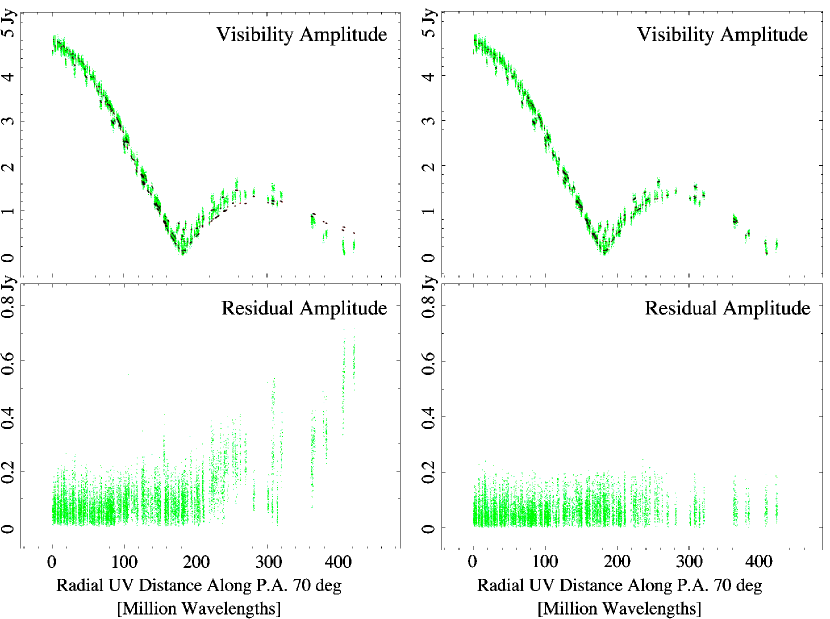
Figure 11.— Visibility amplitudes projected radially along P.A. 70^∘ for the 1996.82 observation of 3C 111. The double-peak indicates the presence of a bright structure within less than a milliarcsecond of the core. The top left panel shows a model (black) which was fitted to the data (green) consisting of one model component for the newly ejected jet feature and the residuals of this model are shown in the bottom left panel. Up to about $600$ mJy of correlated flux density is missing from the model. The right panels show the same data fitted by a model consisting of two components (corresponding to E and F).

Table 1Journal of VLBA 2cm Survey observations of 3C 111 analyzed in this study.

Epoch	Code	$S_{\rm tot}$	rms	$C^{\rm\star}$	$m^{\rm{\dagger}}$
		[Jy]	[mJy/beam]	[mJy/beam]	[%]
1995.27	BK 016	$2.6$	$1.8$	$6.5$
1995.96a	BK 037A	$1.8$	$1.1$	$3.4$
1996.82	BK 37D	$4.8$	$0.5$	$2.1$
1997.19	BK 048	$6.0$	$0.9$	$4.9$
1997.66	BK 052A	$4.1$	$1.6$	$6.4$
1998.18	BK 052B	$2.0$	$2.1$	$5.5$
1999.39	BK 068A	$2.6$	$0.6$	$1.9$
1999.85	BK 068C	$2.4$	$1.2$	$4.1$
2000.49	BT 051	$2.6$	$0.5$	$1.4$	1.5
2001.17	BK 068E	$2.1$	$0.3$	$1.3$
2002.00	BR 077D	$2.2$	$0.3$	$1.1$
2002.19	BR 077I	$2.2$	$0.2$	$0.9$
2002.77	BL 111C	$1.6$	$0.5$	$1.7$	0.6
2003.65	BL 111J	$2.1$	$0.3$	$1.2$	0.3
2004.27a	BL 111L	$1.9$	$0.4$	$1.4$	0.7
2004.80b	BL 111P	$2.7$	$0.3$	$1.0$	0.7
2005.02	BL 123A	$3.0$	$0.5$	$1.8$	0.5
2005.73	BL 123O	$2.4$	$0.3$	$1.2$	0.7
⋆ Lowest contour in Fig. 3
† Degree of polarization (see Fig. 10)
a No data from antenna at Mauna Kea
b No data from antenna at St.Croix

Table 2Model fit parameters

ID	Flux Density [mJy]	Radius [mas]	P.A.a [∘]	FWHM [mas]	ratio	$\phi$[∘]
1995.27
0	1371.04 $\pm$ 205.66	0.00	24.00	0.33 $\pm$ 0.60	0.43	56.22
D	876.06 $\pm$ 131.41	0.61 $\pm$ 0.30	61.18	0.21 $\pm$ 0.54	1.00	–
C	149.59 $\pm$ 22.44	1.14 $\pm$ 0.21	60.80	0.41 $\pm$ 0.64	1.00	–
B	112.85 $\pm$ 16.93	2.06 $\pm$ 0.29	69.41	0.62 $\pm$ 0.79	1.00	–
A	73.30 $\pm$ 10.99	3.97 $\pm$ 0.30	70.69	0.00 $\pm$ 0.50	1.00	–
1995.96
0	1173.64 $\pm$ 176.05	0.00	–	0.35 $\pm$ 0.12	0.59	47.42
D	353.66 $\pm$ 53.05	0.73 $\pm$ 0.30	61.85	0.30 $\pm$ 0.12	1b	–
C	145.60 $\pm$ 21.84	1.72 $\pm$ 0.21	62.73	0.38 $\pm$ 0.13	1b	–
B	46.15 $\pm$ 6.92	3.37 $\pm$ 0.29	70.25	0.61 $\pm$ 0.16	1b	–
A	43.54 $\pm$ 6.53	4.53 $\pm$ 0.30	69.99	-c	1b	–
1996.82
0	1645.03 $\pm$ 246.75	0.00	–	0.26 $\pm$ 0.11	0.17	60.63
F	1608.94 $\pm$ 241.34	0.44 $\pm$ 0.07	54.71	0.31 $\pm$ 0.12	0.19	87.46
E	1344.91 $\pm$ 201.74	0.73 $\pm$ 0.02	67.83	0.23 $\pm$ 0.11	0.61	35.24
X1	121.29 $\pm$ 18.19	1.06 $\pm$ 0.3	61.59	0.33 $\pm$ 0.12	1b	–
C	38.24 $\pm$ 5.74	3.28 $\pm$ 0.21	66.12	0.88 $\pm$ 0.20	1b	–
B	38.04 $\pm$ 5.71	4.76 $\pm$ 0.06	68.08	0.66 $\pm$ 0.16	1b	–
1997.19
0	2490.20 $\pm$ 373.53	0.00	–	0.38 $\pm$ 0.13	0.26	62.36
F	1980.30 $\pm$ 297.05	0.77 $\pm$ 0.07	55.51	0.34 $\pm$ 0.12	0.39	57.52
E	1410.05 $\pm$ 211.51	1.06 $\pm$ 0.02	71.09	0.34 $\pm$ 0.12	0.35	51.00
C	32.15 $\pm$ 4.82	3.72 $\pm$ 0.21	65.48	0.23 $\pm$ 0.11	1b	–
B	35.26 $\pm$ 5.29	5.45 $\pm$ 0.06	67.95	0.72 $\pm$ 0.18	1b	–
1997.66
0	1697.09 $\pm$ 254.56	0.00	–	0.51 $\pm$ 0.14	0c	59.71
F	940.20 $\pm$ 141.03	0.93 $\pm$ 0.07	60.22	0.27 $\pm$ 0.11	1b	–
E	1461.49 $\pm$ 219.22	1.56 $\pm$ 0.02	67.18	0.40 $\pm$ 0.13	1b	–
1998.18
0	1128.63 $\pm$ 169.29	0.00	–	0.82 $\pm$ 0.19	0.47	6.27
F	131.71 $\pm$ 19.76	1.36 $\pm$ 0.07	59.83	0.59 $\pm$ 0.16	1b	–
E	815.70 $\pm$ 122.35	2.07 $\pm$ 0.02	67.53	0.90 $\pm$ 0.21	0.65	11.93
1999.39
0	1509.63 $\pm$ 226.44	0.00	–	0.38 $\pm$ 0.13	0c	64.00
X3	225.98 $\pm$ 33.90	0.59 $\pm$ 0.30	62.46	0.14 $\pm$ 0.10	1b	–
X2	54.38 $\pm$ 8.16	1.25 $\pm$ 0.30	65.08	0.56 $\pm$ 0.15	1b	–
E3	470.42 $\pm$ 70.56	3.51 $\pm$ 0.28	68.80	1.34 $\pm$ 0.29	0.37	57.41
E1	298.52 $\pm$ 44.78	4.21 $\pm$ 0.12	66.02	0.56 $\pm$ 0.15	0.42	35.72
1999.85
0	960.22 $\pm$ 144.03	0.00	–	0.78 $\pm$ 0.19	0.41	-4.69
X4	743.68 $\pm$ 111.55	0.55 $\pm$ 0.30	59.07	1.13 $\pm$ 0.25	0.58	61.59
E3	349.03 $\pm$ 52.35	3.82 $\pm$ 0.28	67.78	1.26 $\pm$ 0.27	0.69	50.04
E2	122.27 $\pm$ 18.34	4.66 $\pm$ 0.21	65.12	0.84 $\pm$ 0.20	0.39	-16.32
E1	267.68 $\pm$ 40.15	5.12 $\pm$ 0.12	64.17	0.84 $\pm$ 0.19	0.40	-7.05
2000.49
0	1668.98 $\pm$ 250.35	0.00	–	0.33 $\pm$ 0.12	0.11	66.21
X7	249.65 $\pm$ 37.45	0.65 $\pm$ 0.30	56.02	0.45 $\pm$ 0.13	1b	–
X6	133.82 $\pm$ 20.07	1.31 $\pm$ 0.30	59.94	0.48 $\pm$ 0.14	1b	–
X5	43.07 $\pm$ 6.46	2.34 $\pm$ 0.30	66.11	0.71 $\pm$ 0.17	1b	–
E4	66.54 $\pm$ 9.98	3.80 $\pm$ 0.15	68.04	0.47 $\pm$ 0.14	1b	–
E3	160.55 $\pm$ 24.08	4.46 $\pm$ 0.28	63.86	0.61 $\pm$ 0.16	1b	–
E2	125.58 $\pm$ 18.84	5.35 $\pm$ 0.21	64.62	0.74 $\pm$ 0.18	1b	–
E1	135.77 $\pm$ 20.37	6.08 $\pm$ 0.12	64.13	0.68 $\pm$ 0.17	1b	–
2001.17
0	1596.68 $\pm$ 239.50	0.00	–	0.44 $\pm$ 0.13	0c	61.41
G	243.56 $\pm$ 36.53	1.13 $\pm$ 0.07	58.96	0.88 $\pm$ 0.20	0.22	54.85
E4	91.23 $\pm$ 13.68	3.96 $\pm$ 0.15	66.28	1.11 $\pm$ 0.24	0.35	48.34
E3	99.76 $\pm$ 14.96	5.21 $\pm$ 0.28	62.80	1.24 $\pm$ 0.27	0.54	65.22
E2	45.34 $\pm$ 6.80	6.20 $\pm$ 0.21	66.06	0.91 $\pm$ 0.21	0.92	55.42
E1	45.18 $\pm$ 6.78	7.20 $\pm$ 0.12	64.16	0.86 $\pm$ 0.20	0.83	75.97
2002.00
0	1514.03 $\pm$ 227.10	0.00	–	0.49 $\pm$ 0.14	0.09	61.18
H	424.80 $\pm$ 63.72	1.02 $\pm$ 0.02	64.67	0.46 $\pm$ 0.14	0.39	66.86
G	60.57 $\pm$ 9.09	2.59 $\pm$ 0.07	58.88	0.94 $\pm$ 0.21	0.33	50.61
E4	121.10 $\pm$ 18.16	4.72 $\pm$ 0.15	64.66	1.40 $\pm$ 0.30	0.35	47.76
E3	19.67 $\pm$ 2.95	5.90 $\pm$ 0.28	65.92	0.82 $\pm$ 0.19	1b	–
E2	21.62 $\pm$ 3.24	6.98 $\pm$ 0.21	64.03	1.12 $\pm$ 0.25	1b	–
E1	24.46 $\pm$ 3.67	8.43 $\pm$ 0.12	65.14	1.04 $\pm$ 0.23	1b	–
2002.19
0	1688.54 $\pm$ 253.28	0.00	–	0.56 $\pm$ 0.15	0.09	63.02
H	317.77 $\pm$ 47.66	1.31 $\pm$ 0.02	64.52	0.48 $\pm$ 0.14	0.56	65.20
G	29.58 $\pm$ 4.44	3.07 $\pm$ 0.07	57.88	-c	1b	–
E4	118.14 $\pm$ 17.72	4.91 $\pm$ 0.15	64.22	1.51 $\pm$ 0.32	0.36	52.47
E3	12.28 $\pm$ 1.84	6.18 $\pm$ 0.28	67.59	0.51 $\pm$ 0.14	1b	–
E2	17.46 $\pm$ 2.62	7.77 $\pm$ 0.21	64.31	1.00 $\pm$ 0.22	1b	–
E1	12.35 $\pm$ 1.85	8.74 $\pm$ 0.12	66.18	0.54 $\pm$ 0.15	1b	–
2002.77
0	1280.01 $\pm$ 192.00	0.00	–	0.47 $\pm$ 0.14	0c	62.23
J	100.40 $\pm$ 15.06	0.61 $\pm$ 0.28	68.62	0.30 $\pm$ 0.12	1b	–
I	78.58 $\pm$ 11.79	1.30 $\pm$ 0.22	61.52	0.34 $\pm$ 0.12	1b	–
H	90.33 $\pm$ 13.55	2.30 $\pm$ 0.02	64.39	0.50 $\pm$ 0.14	1b	–
G	47.49 $\pm$ 7.12	4.16 $\pm$ 0.07	61.40	0.84 $\pm$ 0.20	1b	–
E4	53.64 $\pm$ 8.05	5.51 $\pm$ 0.15	63.49	0.87 $\pm$ 0.20	1b	–
E3	13.63 $\pm$ 2.04	6.85 $\pm$ 0.28	64.21	0.84 $\pm$ 0.20	1b	–
E2	10.84 $\pm$ 1.63	8.51 $\pm$ 0.21	66.27	1.23 $\pm$ 0.27	1b	–
E1	11.31 $\pm$ 1.70	9.69 $\pm$ 0.12	62.75	1.45 $\pm$ 0.31	1b	–
2003.65
0	1046.67 $\pm$ 157.00	0.00	–	0.32 $\pm$ 0.12	0.20	74.73
X9	576.24 $\pm$ 86.44	0.36 $\pm$ 0.30	68.30	0.09 $\pm$ 0.10	1b	–
K	177.19 $\pm$ 26.58	0.69 $\pm$ 0.20	66.00	0.14 $\pm$ 0.10	1b	–
X8	66.75 $\pm$ 10.01	1.30 $\pm$ 0.30	62.77	0.17 $\pm$ 0.11	1b	–
J	34.80 $\pm$ 5.22	1.94 $\pm$ 0.28	63.40	0.33 $\pm$ 0.12	1b	–
I	21.58 $\pm$ 3.24	2.71 $\pm$ 0.22	62.07	0.51 $\pm$ 0.14	1b	–
H	67.76 $\pm$ 10.16	3.86 $\pm$ 0.02	62.83	0.97 $\pm$ 0.22	1b	–
G	64.55 $\pm$ 9.68	5.73 $\pm$ 0.07	60.73	0.59 $\pm$ 0.15	1b	–
E4	7.48 $\pm$ 1.12	6.46 $\pm$ 0.15	60.88	0.57 $\pm$ 0.15	1b	–
E3	13.78 $\pm$ 2.07	7.95 $\pm$ 0.28	65.78	1.59 $\pm$ 0.33	1b	–
E1	11.72 $\pm$ 1.76	10.90 $\pm$ 0.12	63.95	1.79 $\pm$ 0.37	1b	–
2004.27
0	1204.12 $\pm$ 180.62	0.00	–	0.31 $\pm$ 0.12	0.14	70.05
X10	270.09 $\pm$ 40.51	0.44 $\pm$ 0.30	68.51	-c	1b	–
L	105.50 $\pm$ 15.83	0.82 $\pm$ 0.20	69.58	0.20 $\pm$ 0.11	1b	–
K	38.46 $\pm$ 5.77	1.58 $\pm$ 0.20	66.52	0.41 $\pm$ 0.13	1b	–
J	26.88 $\pm$ 4.03	2.42 $\pm$ 0.28	63.12	0.40 $\pm$ 0.13	1b	–
I	11.76 $\pm$ 1.76	3.36 $\pm$ 0.22	65.95	1.09 $\pm$ 0.24	1b	–
H3	110.03 $\pm$ 16.50	4.45 $\pm$ 0.21	63.91	0.45 $\pm$ 0.14	1b	–
H2	76.83 $\pm$ 11.53	4.74 $\pm$ 0.18	59.02	0.35 $\pm$ 0.12	1b	–
H1	26.80 $\pm$ 4.02	5.45 $\pm$ 0.24	62.26	0.82 $\pm$ 0.19	1b	–
G	26.20 $\pm$ 3.93	6.81 $\pm$ 0.07	61.25	1.12 $\pm$ 0.25	1b	–
E4	15.80 $\pm$ 2.37	6.79 $\pm$ 0.15	61.23	0.58 $\pm$ 0.15	1b	–
E3	5.15 $\pm$ 0.77	8.63 $\pm$ 0.28	63.85	0.75 $\pm$ 0.18	1b	–
E2	5.23 $\pm$ 0.78	10.21 $\pm$ 0.21	67.04	1.37 $\pm$ 0.29	1b	–
E1	3.92 $\pm$ 0.59	12.94 $\pm$ 0.46	64.45	0.77 $\pm$ 0.18	1b	–
2004.80
0	1590.66 $\pm$ 238.60	0.00	–	0.28 $\pm$ 0.11	0.38	66.10
N	507.49 $\pm$ 76.12	0.33 $\pm$ 0.15	61.95	0.14 $\pm$ 0.10	1b	–
M	294.28 $\pm$ 44.14	0.56 $\pm$ 0.15	70.23	0.22 $\pm$ 0.11	1b	–
L	34.00 $\pm$ 5.10	1.06 $\pm$ 0.20	65.05	0.30 $\pm$ 0.12	1b	–
K	15.62 $\pm$ 2.34	1.75 $\pm$ 0.20	70.84	0.38 $\pm$ 0.13	1b	–
J	13.76 $\pm$ 2.06	2.55 $\pm$ 0.28	66.12	0.33 $\pm$ 0.12	1b	–
I	20.41 $\pm$ 3.06	3.62 $\pm$ 0.22	64.10	0.62 $\pm$ 0.16	1b	–
H4	41.27 $\pm$ 6.19	4.93 $\pm$ 0.24	63.72	0.64 $\pm$ 0.16	1b	–
H3	88.46 $\pm$ 13.27	5.25 $\pm$ 0.21	62.60	0.87 $\pm$ 0.20	1b	–
H2	97.12 $\pm$ 14.57	5.59 $\pm$ 0.18	59.49	1.10 $\pm$ 0.24	1b	–
H1	13.27 $\pm$ 1.99	6.47 $\pm$ 0.24	61.41	1.82 $\pm$ 0.38	1b	–
G	21.67 $\pm$ 3.25	7.80 $\pm$ 0.07	61.58	0.37 $\pm$ 0.12	1b	–
E3	4.32 $\pm$ 0.65	9.85 $\pm$ 0.28	66.41	0.97 $\pm$ 0.22	1b	–
E1	6.74 $\pm$ 1.01	13.19 $\pm$ 0.46	64.15	0.77 $\pm$ 0.18	1b	–
2005.02
0	1631.40 $\pm$ 244.71	0.00	–	0.24 $\pm$ 0.11	0.21	61.51
N	542.58 $\pm$ 81.39	0.31 $\pm$ 0.15	70.03	0.06 $\pm$ 0.10	1b	–
M	386.90 $\pm$ 58.03	0.67 $\pm$ 0.15	63.61	0.15 $\pm$ 0.10	1b	–
X11	187.02 $\pm$ 28.05	0.86 $\pm$ 0.30	70.85	0.20 $\pm$ 0.11	1b	–
L	17.02 $\pm$ 2.55	1.47 $\pm$ 0.20	67.37	-c	1b	–
K	12.09 $\pm$ 1.81	1.99 $\pm$ 0.20	68.81	0.39 $\pm$ 0.13	1b	–
J	16.23 $\pm$ 2.43	3.21 $\pm$ 0.28	64.59	0.99 $\pm$ 0.22	1b	–
I	12.46 $\pm$ 1.87	4.28 $\pm$ 0.22	64.94	0.54 $\pm$ 0.15	1b	–
H4	101.42 $\pm$ 15.21	5.42 $\pm$ 0.24	62.82	0.47 $\pm$ 0.14	1b	–
H3	58.52 $\pm$ 8.78	5.81 $\pm$ 0.21	59.93	0.39 $\pm$ 0.13	1b	–
H2	46.72 $\pm$ 7.01	6.18 $\pm$ 0.18	59.53	0.79 $\pm$ 0.19	1b	–
H1	4.59 $\pm$ 0.69	7.16 $\pm$ 0.24	61.98	-c	1b	–
G	15.88 $\pm$ 2.38	8.07 $\pm$ 0.07	61.54	0.87 $\pm$ 0.20	1b	–
E3	4.09 $\pm$ 0.61	10.02 $\pm$ 0.28	66.09	1.51 $\pm$ 0.32	1b	–
E1	5.04 $\pm$ 0.76	13.35 $\pm$ 0.46	65.18	1.28 $\pm$ 0.27	1b	–
2005.73
0	1197.32 $\pm$ 179.60	0.00	–	0.28 $\pm$ 0.11	0.30	69.16
X14	480.43 $\pm$ 72.06	0.35 $\pm$ 0.30	70.12	0.12 $\pm$ 0.10	1b	–
X13	224.64 $\pm$ 33.70	0.67 $\pm$ 0.30	68.78	0.13 $\pm$ 0.10	1b	–
N	71.31 $\pm$ 10.70	1.07 $\pm$ 0.15	63.01	0.23 $\pm$ 0.11	1b	–
M	219.35 $\pm$ 32.90	1.86 $\pm$ 0.15	69.54	0.34 $\pm$ 0.12	0.67	41.38
L	13.95 $\pm$ 2.09	2.41 $\pm$ 0.20	65.06	0.29 $\pm$ 0.12	1b	–
K	4.81 $\pm$ 0.72	3.09 $\pm$ 0.20	66.29	-c	1b	–
J	12.38 $\pm$ 1.86	4.32 $\pm$ 0.28	64.25	0.78 $\pm$ 0.18	1b	–
I	12.70 $\pm$ 1.91	5.33 $\pm$ 0.22	64.91	0.85 $\pm$ 0.20	1b	–
H4	32.74 $\pm$ 4.91	6.20 $\pm$ 0.24	61.84	0.46 $\pm$ 0.14	1b	–
H3	38.49 $\pm$ 5.77	6.60 $\pm$ 0.21	60.79	0.53 $\pm$ 0.15	1b	–
H2	35.44 $\pm$ 5.32	7.21 $\pm$ 0.18	58.47	0.84 $\pm$ 0.19	1b	–
H1	13.71 $\pm$ 2.06	8.20 $\pm$ 0.24	63.77	0.88 $\pm$ 0.20	1b	–
G	5.03 $\pm$ 0.75	9.56 $\pm$ 0.07	59.78	0.52 $\pm$ 0.14	1b	–
E3	1.97 $\pm$ 0.30	11.42 $\pm$ 0.28	66.32	-c	1b	–
E1	4.99 $\pm$ 0.75	15.30 $\pm$ 0.46	64.80	2.10 $\pm$ 0.43	1b	–

Table 3Kinematics

References

- Agudo et al. (2001) Agudo, I., Gómez, J., Martí, J. M., et al. 2001, ApJ, 549, L183
- Alef et al. (1998) Alef, W., Preuss, E., Kellermann, K. I., Gabuzda, D. 1998, in Radio Emission from Galactic and Extragalactic Compact Sources, ASP Conf. Ser. 144, 129
- Aller, Aller, & Hughes (2003) Aller, M. F., Aller, H. D., Hughes, P. A. 2003, in Radio Astronomy at the Fringe, Zensus, J. A., Cohen, M. H., Ros, E. (eds.), ASP Conference Ser. 300, 159
- Aloy et al. (2003) Aloy, M.-Á., Martí, J.-M., Gómez, J.-L., Agudo, I., Müller, E., & Ibáñez, J.-M. 2003, ApJ, 585, L109
- Blandford & Konigl (1979) Blandford, R. D., & Konigl, A. 1979, ApJ, 232, 34
- Cara & Lister (2007) Cara, M., & Lister, M. L. 2007, ArXiv Astrophysics e-prints, arXiv:astro-ph/0702449
- Cohen et al. (1971) Cohen, M. H., Cannon, W., Purcell, G. H., Shaffer, D. B., Broderick, J. J., Kellermann, K. I., & Jauncey, D. L. 1971, ApJ, 170, 207
- Cohen et al. (1977) Cohen, M. H., et al. 1977, Nature, 268, 405
- Cohen et al. (2007) Cohen, M. H., Lister, M. L., Homan, D. C., Kadler, M., Kellermann, K. I., Kovalev, Y. Y., & Vermeulen, R. C. 2007, ApJ, 658, 232
- Goetz et al. (1987) Goetz, M. M. A., Preuss, E., Alef, W., & Kellermann, K. I. 1987, A&A, 176, 171
- Gómez et al. (1997) Gómez, J. L., Martí, J. M. A., Marscher, A. P., Ibanez, J. M. A., & Alberdi, A. 1997, ApJ, 482, L33
- Gómez et al. (2001) Gómez, J., Marscher, A. P., Alberdi, A., Jorstad, S. G., Agudo, I. 2001, ApJ, 561, L161
- Gómez (2005) Gómez, J. 2005, Future Directions in High Resolution Astronomy, 340, 13
- Hartman et al. (1999) Hartman, R. C., et al. 1999, ApJS, 123, 79
- Hartman & Kadler (2007) Hartman, R. C. & Kadler, M. 2007, ApJ, submitted
- Homan et al. (2006) Homan, D. C., et al. 2006, ApJ, 642, L115
- Homan & Lister (2006) Homan, D. C., & Lister, M. L. 2006, AJ, 131, 1262
- Homan et al. (2003) Homan, D. C., Lister, M. L., Kellermann, K. I., Cohen, M. H., Ros, E., Zensus, J. A., Kadler, M., & Vermeulen, R. C. 2003, ApJ, 589, L9
- Homan et al. (2002) Homan, D. C., Ojha, R., Wardle, J. F. C., Roberts, D. H., Aller, M. F., Aller, H. D., & Hughes, P. A. 2002, ApJ, 568, 99
- Hughes et al. (1985) Hughes, P. A., Aller, H. D., & Aller, M. F. 1985, ApJ, 298, 301
- Jorstad et al. (2001) Jorstad, S. G., Marscher, A. P., Mattox, J. R., Wehrle, A. E., Bloom, S. D., & Yurchenko, A. V. 2001, ApJS, 134, 181
- Jorstad et al. (2005) Jorstad, S. G., Marscher, A. P., Lister, M. L., et al. 2005, AJ, 130, 1418
- Kadler (2005) Kadler, M. 2005, Ph. D. Thesis, Rheinische Friedrich-Wilhelms-Universität Bonn, Bonn, Germany
- Kadler et al. (2004) Kadler, M., Ros, E., Lobanov, A. P., Falcke, H., Zensus, J. A. 2004, A&A, 426, 481
- Kellermann et al. (1998) Kellermann, K. I., Vermeulen, R. C., Zensus, J. A., & Cohen, M. H. 1998, AJ, 115, 1295
- Kellermann & Moran (2001) Kellermann, K. I., & Moran, J. M. 2001, ARA&A, 39, 457
- Kellermann et al. (2004) Kellermann, K. I., Lister, M. L., Homan, D. C., et al. 2004, ApJ, 609, 539
- Kovalev et al. (2005) Kovalev, Y. Y., Kellermann, K. I., Lister, M. L., et al. 2005, AJ, 130, 2473
- Lähteenmäki & Valtaoja (1999) Lähteenmäki, A. & Valtaoja, E. 1999, ApJ, 521, 493
- Leismann et al. (2005) Leismann, T., Antón, L., Aloy, M. A., Müller, E., Martí, J. M., Miralles, J. A., & Ibáñez, J. M. 2005, A&A, 436, 503
- Lewis et al. (2005) Lewis, K. T., Eracleous, M., Gliozzi, M., et al. 2005, ApJ, 622, 816
- Linfield & Perley (1984) Linfield, R. & Perley, R. 1984, ApJ, 279, 60
- Lister & Homan (2005) Lister, M. L., & Homan, D. C. 2005, AJ, 130, 1389
- Lott et al. (2007) Lott, B., Carson, J., Ciprini, S., Dermer, C. D., Giommi, P., Madejski, G., Lonjou, V., & Reimer, A. 2007, American Institute of Physics Conference Series, 921, 347
- Marscher & Gear (1985) Marscher, A. P., & Gear, W. K. 1985, ApJ, 298, 114
- Marscher et al. (2002) Marscher, A. P., Jorstad, S. G., Gómez, J.-L., Aller, M. F., Teräsranta, H., Lister, M. L., & Stirling, A. M. 2002, Nature, 417, 625
- Marscher (2006) Marscher, A. P. 2006, AN 327, 217
- Mukherjee et al. (2002) Mukherjee, R., Halpern, J., Mirabal, N., & Gotthelf, E. V. 2002, ApJ, 574, 693
- Mimica et al. (2004) Mimica, P., Aloy, M. A., Müller, E., & Brinkmann, W. 2004, A&A, 418, 947
- Mimica et al. (2007) Mimica, P., Aloy, M. A., Müller, E. 2007, A&A, 466, 93
- Mizuno et al. (2007) Mizuno, Y., Hardee, P., & Nishikawa, K.-I. 2007, ApJ, 662, 835
- Perucho et al. (2006) Perucho, M., Lobanov, A.P., Martí, J.M., Hardee, P.E. A&A 456, 493, 2006
- Perucho et al. (2007) Perucho, M., Hanasz, M., Martí, J.M., Miralles, J.A. 2007, Phys. Rev. E, 75, 056312
- Perucho & Lobanov (2007) Perucho, M., & Lobanov, A. P. 2007, A&A, 469, L23
- Perucho & Martí (2007) Perucho, M., & Martí, J.M. 2007, MNRAS, 382, 526
- Piner et al. (2007) Piner, B. G., Mahmud, M., Fey, A. L., & Gospodinova, K. 2007, AJ, 133, 2357
- Preuss, Alef, & Kellermann (1988) Preuss, E., Alef, W., Kellermann, K. I. 1988, in IAU Symp. 129: The Impact of VLBI on Astrophysics and Geophysics, 105
- Roca-Sogorb et al. (2008) Roca-Sogorb, M., Perucho, M., G mez, J.L., Mart , J.M., Ant n, L., Aloy, M.A., Agudo, I. 2008, in proceedings of Extragalactic Jets: Theory and Observation from Radio to Gamma-Ray, eds: T.A. Rector, D.S. de Young, ASP Conference Series, in press
- Scheck et al. (2002) Scheck, L., Aloy, M. A., Martí, J. M., Gómez, J. L., Müller, E. 2002, MNRAS, 331, 615
- Sguera et al. (2005) Sguera, V., Bassani, L., Malizia, A., Dean, A. J., Landi, R., & Stephen, J. B. 2005, A&A, 430, 107
- Shepherd (1997) Shepherd, M. C. 1997, Astronomical Data Analysis Software and Systems VI, 125, 77
- Sreekumar et al. (1999) Sreekumar, P., Bertsch, D. L., Hartman, R. C., Nolan, P. L., & Thompson, D. J. 1999, Astroparticle Physics, 11, 221
- Teräsranta et al. (2004) Teräsranta, H., Achren, J., Hanski, M., et al. 2004, A&A, 427, 769
- Tingay, Preston, & Jauncey (2001) Tingay, S. J., Preston, R. A., & Jauncey, D. L. 2001, AJ, 122, 1697
- Vermeulen & Cohen (1994) Vermeulen, R. C., & Cohen, M. H. 1994, ApJ, 430, 467
- Whitney et al. (1971) Whitney, A. R., et al. 1971, Science, 173, 225
- Zavala & Taylor (2002) Zavala, R. T., & Taylor, G. B. 2002, ApJ, 566, L9
- Zensus (1997) Zensus, J. A. 1997, ARA&A, 35, 607
- Zensus et al. (2002) Zensus, J. A., Ros, E., Kellermann, K. I., et al. 2002, AJ, 124, 662