Neutrino Flavor States and the Quantum Theory of Neutrino Oscillations

Abstract

The standard theory of neutrino oscillations is reviewed, highlighting the main assumptions: the definition of the flavor states, the equal-momentum assumption and the time $=$ distance assumption. It is shown that the standard flavor states are correct approximations of the states that describe neutrinos in oscillation experiments. The equal-momentum assumption is shown to be unnecessary for the derivation of the oscillation probability. The time $=$ distance assumption derives from the wave-packet character of the propagating neutrinos. We present a simple quantum-mechanical wave-packet model which allows us to describe the coherence and localization of neutrino oscillations.

XI Mexican Workshop on Particles and Fields

7-12 November 2007, Tuxtla Gutierrez, Chiapas, Mexico

1 Introduction

The idea of neutrino oscillations was discovered by Bruno Pontecorvo in the late 50s in analogy with $K^{0}$-$\bar{K}^{0}$ oscillations Pontecorvo (1957, 1958). In essence, neutrino oscillations are lepton flavor transitions which depend on the distance and time of neutrino propagation between a source and a detector. This is a quantum-mechanical effect due to neutrino mixing, i.e. the fact that flavor neutrinos are coherent superpositions of massive neutrinos. The oscillations are caused by the interference of the different massive neutrinos, which have different phase velocities.

Since in the late 1950s only one active flavor neutrino was known, the electron neutrino, Pontecorvo invented the concept of a sterile neutrino $\nu_{s}$ Pontecorvo (1968), which does not take part in weak interactions. The muon neutrino was discovered at Brookhaven in 1962 in the first accelerator neutrino experiment of Lederman, Schwartz, Steinberger, et al. Danby et al. (1962), following the independent feasibility estimates of Pontecorvo Pontecorvo (1960) and Schwartz Schwartz (1960). Since then, it became clear that oscillations between different active neutrino flavors are possible if neutrinos are massive and mixed. Indeed, in 1967 Pontecorvo Pontecorvo (1968) discussed the possibility of a depletion of the solar $\nu_{e}$ flux due to $\nu_{e}\to\nu_{\mu}$ (or $\nu_{e}\to\nu_{s}$) transitions before the first measurement in the Homestake experiment Cleveland et al. (1998). In 1969 Gribov and Pontecorvo Gribov and Pontecorvo (1969) discussed solar neutrino oscillations due to $\nu_{e}$–$\nu_{\mu}$ mixing.

The standard theory of neutrino oscillations was developed in 1975–76 by Eliezer and Swift Eliezer and Swift (1976), Fritzsch and Minkowski Fritzsch and Minkowski (1976), Bilenky and Pontecorvo Bilenky and Pontecorvo (1976a, b). In this theory, massive neutrinos are treated as plane waves, having definite energy and momentum. Such a description, however, is not completely consistent, because energy–momentum conservation implies that the creation and detection of massive neutrinos with definite energies and momenta is possible only if all the particles involved in the production and detection processes have definite energies and momenta. The problem is that in this case energy–momentum conservation cannot hold simultaneously for different massive neutrinos and the production and detection of a superposition of different massive neutrinos are forbidden. In order to overcome this problem, it is necessary to treat neutrinos and the other particles participating in the production and detection processes as wave packets, as discussed in section 5.

The plan of this paper is as follows: in section 2 we review the standard theory of neutrino oscillations, highlighting the main assumptions, which are discussed in the following sections; in section 3 we discuss the definition of flavor neutrino states; in section 4 we present a covariant plane-wave theory of neutrino oscillations; in section 5 we discuss the necessity of a wave-packet treatment of neutrino oscillations, in section 6 we present a simple quantum-mechanical wave-packet model of neutrino oscillations, and finally in section 7 we draw our conclusions.

2 Standard Theory of Neutrino Oscillations

Neutrino oscillations are a consequence of neutrino mixing:

$$\nu_{\alpha L}(x)=\sum_{k}U_{\alpha k}\,\nu_{kL}(x)\qquad(\alpha=e,\mu,\tau)\,,$$ (1)

where $\nu_{\alpha L}(x)$ are the left-handed flavor neutrino fields, $\nu_{kL}(x)$ are the left-handed massive neutrino fields and $U$ is the unitary mixing matrix (see Refs. Bilenky and Pontecorvo (1978); Bilenky and Petcov (1987); Bilenky et al. (1999); Alberico and Bilenky (2004); Giunti and Kim (2007)). Since a flavor neutrino $\nu_{\alpha}$ is created by $\nu_{\alpha L}^{\dagger}(x)$ in a charged-current weak interaction process, in the standard plane-wave theory of neutrino oscillations Eliezer and Swift (1976); Fritzsch and Minkowski (1976); Bilenky and Pontecorvo (1976a, b, 1978), it is assumed that $\nu_{\alpha}$ is described by the standard flavor state

$$|\nu_{\alpha}\rangle=\sum_{k}U_{\alpha k}^{*}\,|\nu_{k}\rangle\,,$$ (2)

which has the same mixing as the field $\nu_{\alpha L}^{\dagger}(x)$.

Since the massive neutrino states $|\nu_{k}\rangle$ have definite mass $m_{k}$ and definite energy $E_{k}$, they evolve in time as plane waves:

$$i\,\frac{\partial}{\partial t}\,|\nu_{k}(t)\rangle=\mathsf{H}_{0}\,|\nu_{k}(t)\rangle=E_{k}\,|\nu_{k}(t)\rangle\,,\qquad|\nu_{k}(t)\rangle=e^{-iE_{k}t}\,|\nu_{k}\rangle\,,$$ (3)

where $\mathsf{H}_{0}$ is the free Hamiltonian operator,

$$E_{k}^{2}=p_{k}^{2}+m_{k}^{2}\,,$$ (4)

and $|\nu_{k}(t=0)\rangle=|\nu_{k}\rangle$ (all the massive neutrinos start with the same arbitrary phase). The resulting time evolution of the flavor neutrino state in Eq. (2) is given by

$$|\nu_{\alpha}(t)\rangle=\sum_{k}U_{\alpha k}^{*}\,e^{-iE_{k}t}\,|\nu_{k}\rangle=\sum_{\beta=e,\mu,\tau}\left(\sum_{k}U_{\alpha k}^{*}\,e^{-iE_{k}t}\,U_{\beta k}\right)|\nu_{\beta}\rangle\,.$$ (5)

Hence, if the mixing matrix $U$ is different from unity (i.e. if there is neutrino mixing), the state $|\nu_{\alpha}(t)\rangle$, which has pure flavor $\alpha$ at the initial time $t=0$, evolves in time into a superposition of different flavors. The quantity in parentheses in Eq. (5) is the amplitude of $\nu_{\alpha}\to\nu_{\beta}$ transitions at the time $t$ after $\nu_{\alpha}$ production. The probability of $\nu_{\alpha}\to\nu_{\beta}$ transitions at the time $t=T$ of neutrino detection is given by

$$P_{\alpha\beta}(T)=|\langle\nu_{\beta}|\nu_{\alpha}(T)\rangle|^{2}=\left|\sum_{k}U_{\alpha k}^{*}\,e^{-iE_{k}T}\,U_{\beta k}\right|^{2}=\sum_{k,j}U_{\alpha k}^{*}\,U_{\beta k}\,U_{\alpha j}\,U_{\beta j}^{*}\,e^{-i(E_{k}-E_{j})T}\,.$$ (6)

One can see that $P_{\alpha\beta}(T)$ depends on the energy differences $E_{k}-E_{j}$. In the standard theory of neutrino oscillations it is assumed that all massive neutrinos have the same momentum $\vec{p}$. Since detectable neutrinos are ultrarelativistic, we have

$$E_{k}\simeq E+\frac{m_{k}^{2}}{2E}\,,\qquad E_{k}-E_{j}=\frac{\Delta{m}^{2}_{kj}}{2E}\,,$$ (7)

where $\Delta{m}^{2}_{kj}\equiv m_{k}^{2}-m_{j}^{2}$ and $E\equiv|\vec{p}|$ is the energy of a massless neutrino (or, in other words, the neutrino energy in the massless approximation). In most neutrino oscillation experiments the time $T$ between production and detection is not measured, but the source-detector distance $L$ is known. In this case, in order to apply the oscillation probability to the data analysis it is necessary to express $T$ as a function of $L$. Considering ultrarelativistic neutrinos, we have $T\simeq L$, leading to the standard formula for the oscillation probability:

$$P_{\alpha\beta}(L,E)=\sum_{k,j}U_{{\alpha}k}^{*}\,U_{{\beta}k}\,U_{{\alpha}j}\,U_{{\beta}j}^{*}\,\exp\left(-i\,\frac{\Delta{m}^{2}_{kj}L}{2E}\right)\,.$$ (8)

Summarizing, there are three main assumptions in the standard theory of neutrino oscillations:

1. Neutrinos produced or detected in charged-current weak interaction processes are described by the flavor states in Eq. (2).

2. The massive neutrino states $|\nu_{k}\rangle$ in Eq. (2) have the same momentum (“equal-momentum assumption”).

3. The propagation time is equal to the distance $L$ traveled by the neutrino between production and detection (“time $=$ distance assumption”).

In the following we will show that the assumptions (A1) and  (A3) correspond to approximations which are appropriate in the analysis of current neutrino oscillation experiments (section 3 and 5, respectively). Instead, the equal-momentum assumption (A2) is not physically justified Winter (1981); Giunti et al. (1991); Giunti and Kim (2001a); Giunti (2001a, 2004a), as one can easily understand from the application of energy-momentum conservation to the production process. However, in section 4 we will show that the assumption (A2) is actually not necessary for the derivation of the oscillation probability if both the evolutions in space and in time of the neutrino state are taken into account.

3 Flavor Neutrino States

The state of a flavor neutrino $\nu_{\alpha}$ is defined as the state which describes a neutrino produced in a charged-current weak interaction process together with a charged lepton $\ell_{\alpha}^{+}$ or from a charged lepton $\ell_{\alpha}^{-}$ ($\ell_{\alpha}^{\pm}=e^{\pm},\mu^{\pm},\tau^{\pm}$ for $\alpha=e,\mu,\tau$, respectively), or the state which describes a neutrino detected in a charged-current weak interaction process with a charged lepton $\ell_{\alpha}^{-}$ in the final state. In fact, the neutrino flavor can only be measured through the identification of the charged lepton associated with the neutrino in a charged-current weak interaction process.

Let us first consider a neutrino produced in the generic decay process

$$\text{P}_{\text{I}}\to\text{P}_{\text{F}}+\ell_{\alpha}^{+}+\nu_{\alpha}\,,$$ (9)

where $\text{P}_{\text{I}}$ is the decaying particle and $\text{P}_{\text{F}}$ represents any number of final particles. For example: in the pion decay process $\pi^{+}\to\mu^{+}+\nu_{\mu}$ we have $\text{P}_{\text{I}}=\pi^{+}$, $\text{P}_{\text{F}}$ is absent and $\alpha=\mu$; in a nuclear $\beta^{+}$ decay process $\text{N}(A,Z)\to\text{N}(A,Z-1)+e^{+}+\nu_{e}$ we have $\text{P}_{\text{I}}=\text{N}(A,Z)$, $\text{P}_{\text{F}}=\text{N}(A,Z-1)$ and $\alpha=e$. The following method can easily be modified in the case of a $\nu_{\alpha}$ produced in the generic scattering process $\ell_{\alpha}^{-}+\text{P}_{\text{I}}\to\text{P}_{\text{F}}+\nu_{\alpha}$ by replacing the $\ell_{\alpha}^{+}$ in the final state with a $\ell_{\alpha}^{-}$ in the initial state.

The final state resulting from the decay of the initial particle $\text{P}_{\text{I}}$ is given by

$$|f\rangle=\mathsf{S}\,|\text{P}_{\text{I}}\rangle\,,$$ (10)

where $\mathsf{S}$ is the $S$-matrix operator. Since the final state $|f\rangle$ contains all the decay channels of $\text{P}_{\text{I}}$, it can be written as

$$|f\rangle=\sum_{k}\mathcal{A}^{\text{P}}_{\alpha k}\,|\nu_{k},\ell_{\alpha}^{+},\text{P}_{\text{F}}\rangle+\ldots\,,$$ (11)

where we have singled out the decay channel in Eq. (9) and we have taken into account that the flavor neutrino $\nu_{\alpha}$ is a coherent superposition of massive neutrinos $\nu_{k}$. Since the states of the other decay channels represented by dots in Eq. (11) are orthogonal to $|\nu_{k},\ell_{\alpha}^{+},\text{P}_{\text{F}}\rangle$ and the states $|\nu_{k},\ell_{\alpha}^{+},\text{P}_{\text{F}}\rangle$ with different $k$s are orthonormal, the coefficients $\mathcal{A}^{\text{P}}_{\alpha k}$ are the amplitudes of production of the corresponding state in the decay channel in Eq. (9):

$$\mathcal{A}^{\text{P}}_{\alpha k}=\langle\nu_{k},\ell_{\alpha}^{+},\text{P}_{\text{F}}|f\rangle=\langle\nu_{k},\ell_{\alpha}^{+},\text{P}_{\text{F}}|\,\mathsf{S}\,|\text{P}_{\text{I}}\rangle\,.$$ (12)

Projecting the final state in Eq. (11) over $|\ell_{\alpha}^{+},\text{P}_{\text{F}}\rangle$ and normalizing, we obtain the flavor neutrino state Giunti et al. (1992); Bilenky and Giunti (2001); Alberico and Bilenky (2004); Giunti (2004b)

$$|\nu_{\alpha}^{\text{P}}\rangle=\left(\sum_{i}|\mathcal{A}^{\text{P}}_{\alpha i}|^{2}\right)^{-1/2}\sum_{k}\mathcal{A}^{\text{P}}_{\alpha k}\,|\nu_{k}\rangle\,.$$ (13)

Therefore, a flavor neutrino state is a coherent superposition of massive neutrino states $|\nu_{k}\rangle$ and the coefficient $\mathcal{A}^{\text{P}}_{\alpha k}$ of the $k$th massive neutrino component is given by the amplitude of production of $\nu_{k}$. Since, in general, the amplitudes $\mathcal{A}^{\text{P}}_{\alpha k}$ depend on the production process, a flavor neutrino state depends on the production process. In the following, we will call a flavor neutrino state of the type in Eq. (13) a “production flavor neutrino state”.

Let us now consider the detection of a flavor neutrino $\nu_{\alpha}$ through the generic charged-current weak interaction process

$$\nu_{\alpha}+\text{D}_{\text{I}}\to\text{D}_{\text{F}}+\ell_{\alpha}^{-}\,,$$ (14)

where $\text{D}_{\text{I}}$ is the target particle and $\text{D}_{\text{F}}$ represents one or more final particles. In general, since the incoming neutrino state in the detection process is a superposition of massive neutrino states, it may not have a definite flavor. Therefore, we must consider the generic process

$$\nu+\text{D}_{\text{I}}\,,$$ (15)

with a generic incoming neutrino state $|\nu\rangle$. In this case, the final state of the scattering process is given by

$$|f\rangle=\mathsf{S}\,|\nu,\text{D}_{\text{I}}\rangle\,,$$ (16)

This final state contains all the possible scattering channels:

$$|f\rangle=|\text{D}_{\text{F}},\ell_{\alpha}^{-}\rangle+\ldots\,,$$ (17)

where we have singled out the scattering channel in Eq. (14). We want to find the component

$$|\nu_{\alpha},\text{D}_{\text{I}}\rangle=\sum_{k}\mathcal{A}^{\text{D}}_{\alpha k}|\nu_{k},\text{D}_{\text{I}}\rangle$$ (18)

of the initial state $|\nu,\text{D}_{\text{I}}\rangle$ which corresponds to the flavor $\alpha$, i.e. the component which generates only the scattering channel in Eq. (14). This means that $|\text{D}_{\text{F}},\ell_{\alpha}^{-}\rangle=\mathsf{S}\,|\nu_{\alpha},\text{D}_{\text{I}}\rangle$. Using the unitarity of the mixing matrix, we obtain

$$|\nu_{\alpha},\text{D}_{\text{I}}\rangle=\mathsf{S}^{\dagger}\,|\text{D}_{\text{F}},\ell_{\alpha}^{-}\rangle\,.$$ (19)

From Eqs. (18) and (19), the coefficients $\mathcal{A}^{\text{D}}_{\alpha k}$ are the complex conjugate of the amplitude of detection of $\nu_{k}$ in the detection process in Eq. (14):

$$\mathcal{A}^{\text{D}}_{\alpha k}=\langle\nu_{k},\text{D}_{\text{I}}|\mathsf{S}^{\dagger}\,|\text{D}_{\text{F}},\ell_{\alpha}^{-}\rangle\,.$$ (20)

Projecting $|\nu_{\alpha},\text{D}_{\text{I}}\rangle$ over $|\text{D}_{\text{I}}\rangle$ and normalizing, we finally obtain the flavor neutrino state in the detection process in Eq. (14):

$$|\nu_{\alpha}^{\text{D}}\rangle=\left(\sum_{i}|\mathcal{A}^{\text{D}}_{\alpha i}|^{2}\right)^{-1/2}\sum_{k}\mathcal{A}^{\text{D}}_{\alpha k}\,|\nu_{k}\rangle\,.$$ (21)

In the following, we will call a flavor neutrino state of this type a “detection flavor neutrino state”.

Although the expressions in Eqs. (13) and (21) for the production and detection flavor neutrino states have the same structure, these states have different meanings. A production flavor neutrino state describes the neutrino created in a charged-current interaction process, which propagates out of a source. Hence, it describes the initial state of a propagating neutrino. A detection flavor neutrino state does not describe a propagating neutrino. It describes the component of the state of a propagating neutrino which can generate a charged lepton with appropriate flavor through a charged-current weak interaction with an appropriate target particle. In other words, the scalar product

$$A_{\alpha}=\langle\nu_{\alpha}^{\text{D}}|\nu\rangle$$ (22)

is the probability amplitude to find a $\nu_{\alpha}$ by observing the scattering channel in Eq. (14) with the scattering process in Eq. (15).

In order to understand the connection of the production and detection flavor neutrino states with the standard flavor neutrino states in Eq. (2), it is useful to express the $S$-matrix operator as

$$\mathsf{S}=1-i\int\text{d}^{4}x\,\mathsf{H}_{\text{CC}}(x)\,,\qquad\mathsf{H}_{\text{CC}}(x)=\frac{G_{\text{F}}}{\sqrt{2}}\,j_{\rho}^{\dagger}(x)\,j^{\rho}(x)\,,$$ (23)

where $G_{\text{F}}$ is the Fermi constant (we considered only the first order perturbative contribution of the effective low-energy charged-current weak interaction Hamiltonian). The weak charged current $j^{\rho}(x)$ is given by

$$j^{\rho}(x)=\hbox{} \hbox{}\sum_{\alpha=e,\mu,\tau}\overline{\nu_{\alpha}}(x)\,\gamma^{\rho}\left(1-\gamma^{5}\right)\ell_{\alpha}(x)+h^{\rho}(x)$$

$$=\hbox{} \hbox{}\sum_{\alpha=e,\mu,\tau}\sum_{k}U_{\alpha k}^{*}\,\overline{\nu_{k}}(x)\,\gamma^{\rho}\left(1-\gamma^{5}\right)\ell_{\alpha}(x)+h^{\rho}(x)\,,$$ (24)

where $h^{\rho}(x)$ is the hadronic weak charged current. The production and detection amplitudes $\mathcal{A}^{\text{P}}_{\alpha k}$ and $\mathcal{A}^{\text{D}}_{\alpha k}$ can be written as

$$\mathcal{A}^{\text{P}}_{\alpha k}=U_{\alpha k}^{*}\,\mathcal{M}^{\text{P}}_{\alpha k}\,,\qquad\mathcal{A}^{\text{D}}_{\alpha k}=U_{\alpha k}^{*}\,\mathcal{M}^{\text{D}}_{\alpha k}\,,$$ (25)

with the interaction matrix elements

$$\hbox{}\mathcal{M}^{\text{P}}_{\alpha k}=-i\,\frac{G_{\text{F}}}{\sqrt{2}}\int\text{d}^{4}x\,\langle\nu_{k},\ell_{\alpha}^{+}|\,\overline{\nu_{k}}(x)\,\gamma^{\rho}\left(1-\gamma^{5}\right)\ell_{\alpha}(x)\,|0\rangle\,J_{\rho}^{\text{P}_{\text{I}}\to\text{P}_{\text{F}}}(x)\,,$$ (26)

$$\hbox{}\mathcal{M}^{\text{D}}_{\alpha k}=i\,\frac{G_{\text{F}}}{\sqrt{2}}\int\text{d}^{4}x\,\langle\nu_{k}|\,\overline{\nu_{k}}(x)\,\gamma^{\rho}\left(1-\gamma^{5}\right)\ell_{\alpha}(x)\,|\ell_{\alpha}^{-}\rangle\,{J_{\rho}^{\text{D}_{\text{I}}\to\text{D}_{\text{F}}}}^{*}(x)\,.$$ (27)

Here $J_{\rho}^{\text{P}_{\text{I}}\to\text{P}_{\text{F}}}(x)$ and $J_{\rho}^{\text{D}_{\text{I}}\to\text{D}_{\text{F}}}(x)$ are, respectively, the matrix elements of the $\text{P}_{\text{I}}\to\text{P}_{\text{F}}$ and $\text{D}_{\text{I}}\to\text{D}_{\text{F}}$ transitions.

Using Eq. (25), the production and detection flavor neutrino states can be written as

$$\hbox{}|\nu_{\alpha}^{\text{P}}\rangle=\sum_{k}\frac{\mathcal{M}^{\text{P}}_{\alpha k}}{\sqrt{\sum_{j}|U_{\alpha j}|^{2}\,|\mathcal{M}^{\text{P}}_{\alpha j}|^{2}}}\,U_{\alpha k}^{*}\,|\nu_{k}\rangle\,,$$ (28)

$$\hbox{}|\nu_{\alpha}^{\text{D}}\rangle=\sum_{k}\frac{\mathcal{M}^{\text{D}}_{\alpha k}}{\sqrt{\sum_{j}|U_{\alpha j}|^{2}\,|\mathcal{M}^{\text{D}}_{\alpha j}|^{2}}}\,U_{\alpha k}^{*}\,|\nu_{k}\rangle\,.$$ (29)

These states have a structure which is similar to the standard flavor states in Eq. (2), with the relative contribution of the massive neutrino $\nu_{k}$ proportional to $U_{\alpha k}^{*}$. The additional factors are due to the dependence of the production and detection processes on the neutrino masses.

In experiments which are not sensitive to the dependence of $\mathcal{M}^{\text{P}}_{\alpha k}$ and $\mathcal{M}^{\text{D}}_{\alpha k}$ on the difference of the neutrino masses, it is possible to approximate

$$\mathcal{M}^{\text{P}}_{\alpha k}\simeq\mathcal{M}^{\text{P}}_{\alpha}\,,\qquad\mathcal{M}^{\text{D}}_{\alpha k}\simeq\mathcal{M}^{\text{D}}_{\alpha}\,.$$ (30)

In this case, since

$$\sum_{k}|U_{\alpha k}|^{2}=1\,,$$ (31)

we obtain, up to an irrelevant phase, the standard flavor neutrino states in Eq. (2), which do not depend on the production or detection process. Hence, the standard flavor neutrino states are approximations of the production and detection flavor neutrino states in experiments which are not sensitive to the dependence of the neutrino interaction rate on the difference of the neutrino masses. All neutrino oscillation experiments have this characteristic: since the detectable neutrinos are ultrarelativistic, neutrino oscillation experiments are insensitive to any effect of neutrino masses in the production and detection processes. Therefore, the assumption (A1) in the standard theory of neutrino oscillations is correct as an appropriate approximation in the analysis of neutrino oscillation experiments.

4 Covariant Plane-Wave Theory of Oscillations

In this section we show that the equal-momentum assumption (A2) can be avoided by considering not only the time evolution of the neutrino states, as in the standard theory, but also their space dependence.

Let us consider a neutrino oscillation experiment in which $\nu_{\alpha}\to\nu_{\beta}$ transitions are studied with a production process of the type in Eq. (9) and a detection process of the type in Eq. (14). In this case, the produced flavor neutrino $\nu_{\alpha}$ is described by the production flavor state $|\nu_{\alpha}^{\text{P}}\rangle$ in Eq. (13). If the neutrino production and detection processes are separated by a space-time interval $(T,L)$, the neutrino propagates freely between production and detection, evolving into the state

$$|\nu(T,L)\rangle=e^{-i\mathsf{E}T+i\mathsf{P}L}\,|\nu_{\alpha}^{\text{P}}\rangle\,,$$ (32)

where $\mathsf{E}\equiv\mathsf{H}_{0}$ and $\mathsf{P}$ are, respectively, the energy and momentum operators. This is the incoming neutrino state in the detection process. The amplitude of the measurable $\nu_{\alpha}\to\nu_{\beta}$ transitions is given by the scalar product in Eq. (22):

$$A_{\alpha\beta}(T,L)=\langle\nu_{\beta}^{\text{D}}|\nu(T,L)\rangle=\langle\nu_{\beta}^{\text{D}}|e^{-i\mathsf{E}T+i\mathsf{P}L}|\nu_{\alpha}^{\text{P}}\rangle\,,$$ (33)

with the detection flavor state $|\nu_{\beta}^{\text{D}}\rangle$ in Eq. (21).

Neglecting mass effects in the production and detection processes, we approximate the production and detection flavor states with the standard ones given in Eq. (2). Then, we obtain

$$A_{\alpha\beta}(T,L)=\sum_{k}U_{\alpha k}^{*}\,U_{\beta k}\,e^{-iE_{k}T+ip_{k}L}\,.$$ (34)

Notice that the consideration of the space-time interval between neutrino production and detection allows one to take into account both the differences in energy and momentum of the massive neutrinos Winter (1981); Giunti et al. (1991); Giunti and Kim (2001a); Giunti (2001a, 2004a).

In oscillation experiments in which the neutrino propagation time $T$ is not measured, it is possible to adopt the light-ray $T=L$ approximation (assumption (A3)), since neutrinos are ultrarelativistic (the effects of possible deviations from $T=L$ are shown to be negligible in Refs. Giunti (2007); Giunti and Kim (2007)). In this case, the phase in Eq. (34) becomes

$$-E_{k}T+p_{k}L=-\left(E_{k}-p_{k}\right)L=-\frac{E_{k}^{2}-p_{k}^{2}}{E_{k}+p_{k}}\,L=-\frac{m_{k}^{2}}{E_{k}+p_{k}}\,L\simeq-\frac{m_{k}^{2}}{2E}\,L\,,$$ (35)

which leads to the standard oscillation probability in Eq. (8).

Equation (35) shows that the phases in the flavor transition amplitude are independent from the values of the energies and momenta of different massive neutrinos Winter (1981); Giunti et al. (1991); Giunti and Kim (2001a); Giunti (2001a, 2004a), because of the relativistic dispersion relation in Eq. (4). In particular, Eq. (35) shows that the equal-momentum assumption (A2) in section 2, adopted in the standard derivation of the neutrino oscillation probability, is not necessary in an improved derivation which takes into account both the evolutions in space and in time of the neutrino state.

We have called this derivation of the flavor transition probability “covariant plane-wave theory of oscillations” because it is manifestly Lorentz invariant. This is important because flavor, which is the quantum number that distinguishes different types of quarks and leptons, is a Lorentz-invariant quantity. For example, an electron is seen as an electron by any observer, never as a muon. Therefore, the probability of flavor neutrino oscillations must be Lorentz invariant Giunti and Kim (2001a); Giunti (2004c).

5 Wave-Packet Treatment

So far, we have considered massive neutrinos as particles described by plane waves with definite energy and momentum. However, the $T=L$ assumption (A3) requires a wave packet description. The reason is simple: since plane waves cover all space-time in a periodic way they cannot describe the localized events of neutrino production and detection. As discussed in introductory books on optics (see Born and Wolf (1959); Jenkins and White (1981)) and quantum mechanics (see Schiff (1955); Bohm (1959)), real localized particles are described by superpositions of plane waves known as wave packets.

Moreover, different massive neutrinos can be produced and detected coherently only if the energies and momenta in the production and detection processes have sufficiently large uncertainties Kayser (1981); Kiers et al. (1996). The uncertainty of the production process implies that the massive neutrinos propagating between production and detection have a momentum distribution Giunti (2002a), i.e. they are described by wave packets.

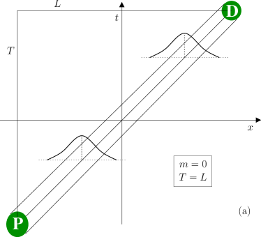
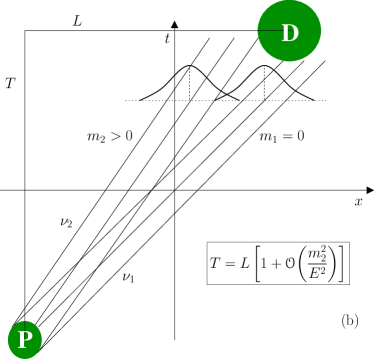
Figure 1: Space-time diagram representing schematically the propagation of the wave packet of a massless particle (a) and the propagation of the wave packets of a superposition of a massless and a massive ultrarelativistic particle (b) from a production process P to a detection process D.

The propagation of a massless particle between localized production and detection processes separated by $T\simeq L$ is illustrated schematically in the space-time diagram in Fig. 1a. The interesting case of propagation of a superposition of two neutrinos with definite masses, one massless ($\nu_{1}$) and one massive but ultrarelativistic ($\nu_{2}$) is illustrated schematically in Fig. 1b. One can note that in these diagrams both the production and detection processes occupy a finite region in space-time, called the coherence region, in which the propagating particles are produced or detected coherently. Indeed, the uncertainty principle implies that any interaction process $I$ has a space uncertainty $\sigma_{x}^{\text{I}}$ related to the momentum uncertainty $\sigma_{p}^{\text{I}}$ by

$$\sigma_{x}^{\text{I}}\,\sigma_{p}^{\text{I}}\sim\frac{1}{2}\,.$$ (36)

A point-like process would have an infinite momentum uncertainty and a process with definite momentum would be completely delocalized in space. The momentum uncertainty can be estimated as the quadratic sum of the uncertainties of the momenta of the localized particles taking part in the process:

$$(\sigma_{p}^{\text{I}})^{2}\sim\sum_{i}(\sigma_{p}^{i})^{2}\,.$$ (37)

The sum is over the initial particles and the final particles which are localized through interaction with the environment. Their momentum uncertainties $\sigma_{p}^{i}$ are related to the size $\sigma_{x}^{i}$ of their wave packets by uncertainty relations analogous to Eq. (36),

$$\sigma_{x}^{i}\,\sigma_{p}^{i}\sim\frac{1}{2}\,.$$ (38)

Therefore, the space uncertainty of the process is given by

$$(\sigma_{x}^{\text{I}})^{-2}\sim\sum_{i}(\sigma_{x}^{i})^{-2}\,.$$ (39)

It is clear that the particle with larger momentum uncertainty and associated smaller space uncertainty gives the dominant contribution.

The coherence time $\sigma_{t}^{\text{I}}$ of an interaction process $I$ is the time over which the wave packets of the interacting particles overlap. If the process is the decay of a particle in vacuum, the localization of such particle and its decay products is very poor and the coherence time $\sigma_{t}^{\text{I}}$ is of the order of the particle lifetime. On the other hand, if the decay occurs in a medium where the decaying particle and its products are well localized or if the production process is a scattering process, the coherence time can be estimated by

$$(\sigma_{t}^{\text{I}})^{-2}\sim\sum_{i}\left(\frac{\sigma_{x}^{i}}{v_{i}}\right)^{-2}\,,$$ (40)

where $v_{i}$ is the velocity of the particle $i$, because $\sigma_{t}^{\text{I}}$ must be dominated by the particle with smaller ratio $\sigma_{x}^{i}/v_{i}$, which is the first to leave the interaction region. Therefore, in general $\sigma_{t}^{\text{I}}\gtrsim\sigma_{x}^{\text{I}}$, in agreement with the physical expectation that the coherence region of a process must be causally connected.

As illustrated in Fig. 1, one can estimate the size of the wave packet of a massive neutrino created in a production process P as the coherence time $\sigma_{t}^{\text{P}}$ of the production process,

$$\sigma_{x}^{\nu}\sim\sigma_{t}^{\text{P}}\,.$$ (41)

Let us emphasize that there is a profound difference between the behavior of final neutrinos and other particles in the production process. The initial particles have wave packets which are determined by their creation process or by previous interactions. The initial particles and the final particles which interact with the environment contribute to the coherence time $\sigma_{t}^{\text{P}}$ through their contribution to the momentum uncertainty in Eq. (37). An initial decaying particle contributes directly to the coherence time $\sigma_{t}^{\text{P}}$ with its lifetime. On the other hand, neutrinos are stable and leave the production process without interacting with the environment. Therefore, they do not contribute to the determination of the coherence time $\sigma_{t}^{\text{P}}$ and the size of their wave packets is determined by $\sigma_{t}^{\text{P}}$.

Considering now the detection process $D$, if there is only one particle propagating between the production and detection processes, as shown in Fig. 1a, the coherence size of the detection process is determined by Eq. (37), with the sum over all the participating particles which interact with the environment and the propagating particle, which is described by a wave packet. In the case of neutrino mixing, the neutrino propagating between the production and detection processes is in general a superposition of massive neutrino wave packets which propagate with different phase velocity, as illustrated in Fig. 1b. In this case, in the detection process, the wave packets of different massive neutrinos are separated by a distance $\Delta{x}=\Delta{v}\,T$, where $\Delta{v}$ is the velocity difference. If the source–detector distance is very large, the separation of the massive neutrino wave packets at detection may be larger than their size, leading to the lack of overlap Nussinov (1976). In this case, the effective coherence size of the neutrino wave function at the detection process is

$$\sigma_{x,\text{eff}}^{\nu}\sim\sqrt{(\sigma_{x}^{\nu})^{2}+(\Delta{x})^{2}}\sim\sqrt{(\sigma_{t}^{\text{P}})^{2}+(\Delta{v}\,T)^{2}}\,.$$ (42)

However, Eq. (39) shows that the particle with smaller space uncertainty gives the dominant contribution to the coherence size of the detection process. Therefore, if the effective coherence size in Eq. (42) of the neutrino wave function is dominated by the separation of the wave packets ($\Delta{v}\,T\gg\sigma_{t}^{\text{P}}$) and there is another particle participating in the detection process which has much smaller space uncertainty, the different massive neutrinos cannot be detected coherently. In this case, there cannot be any interference between the different massive neutrino contributions to the detection process and the probability of transitions between different flavors reduces to the incoherent transition probability

$$P_{\alpha\beta}^{\text{incoherent}}=\sum_{k}|U_{{\alpha}k}|^{2}\,|U_{{\beta}k}|^{2}\,,$$ (43)

which does not oscillate as a function of the source–detector distance. On the other hand, if all the other particles participating in the detection process have space uncertainties which are larger than effective coherence size in Eq. (42) of the neutrino wave function, the different massive neutrinos are detected coherently Kiers et al. (1996), leading to the interference of their contributions to the detection process which manifests itself as oscillations of the probability of flavor transitions, according to Eq. (8).

These considerations show that a wave-packet treatment of massive neutrinos is important in order to understand the coherence properties of neutrino oscillations.

6 Quantum-Mechanical Wave-Packet Model

In this section we present a simple one-dimensional quantum-mechanical wave-packet model Giunti et al. (1991); Giunti and Kim (1998) in which the momentum uncertainties of the states which describe the produced and detected massive neutrinos are approximated by Gaussian distributions. More complete three-dimensional models in which the neutrino momentum uncertainties are obtained from a quantum field theoretical calculation of the production and detection processes are discussed in Refs. Giunti et al. (1993, 1998); Kiers and Weiss (1998); Cardall (2000); Beuthe (2002); Giunti (2002a).

Neglecting mass effects in the production and detection processes, we describe the produced and detected neutrinos in a $\nu_{\alpha}\to\nu_{\beta}$ experiment with the wave-packet flavor states

$$|\nu_{\alpha}^{\text{P}}\rangle=\sum_{k}U_{\alpha k}^{*}\int\mathrm{d}p\,\psi^{\text{P}}_{k}(p)\,|\nu_{k}(p)\rangle\,,\qquad|\nu_{\beta}^{\text{D}}\rangle=\sum_{k}U_{\beta k}^{*}\int\mathrm{d}p\,\psi^{\text{D}}_{k}(p)\,|\nu_{k}(p)\rangle\,,$$ (44)

with the Gaussian momentum distributions

$$\psi^{\text{P}}_{k}(p)=\frac{1}{\left(2\pi(\sigma_{p}^{\text{P}})^{2}\right)^{\frac{1}{4}}}\exp\left[-\frac{\left(p-p_{k}\right)^{2}}{4(\sigma_{p}^{\text{P}})^{2}}\right]\,,\quad\psi^{\text{D}}_{k}(p)=\frac{1}{\left(2\pi(\sigma_{p}^{\text{D}})^{2}\right)^{\frac{1}{4}}}\exp\left[-\frac{\left(p-p_{k}\right)^{2}}{4(\sigma_{p}^{\text{D}})^{2}}\right]\,.$$ (45)

The average momenta $p_{k}$ of the massive neutrinos are determined by the kinematics of the production process. They are the same in the detection process because of causality. On the other hand, the energy-momentum uncertainties in the production and detection processes, $\sigma_{p}^{\text{P}}$ and $\sigma_{p}^{\text{D}}$, may be quite different.

The flavor transition amplitude is given by

$$A_{\alpha\beta}(T,L)=\hbox{} \hbox{}\langle\nu_{\beta}^{\text{D}}|\,e^{-i\mathsf{E}T+i\mathsf{P}L}\,|\nu_{\alpha}^{\text{P}}\rangle$$

$$\propto\hbox{} \hbox{}\sum_{k}U_{\alpha k}^{*}\,U_{\beta k}\,\int\mathrm{d}p\,\exp\left[-iE_{k}(p)T+ipL-\frac{\left(p-p_{k}\right)^{2}}{4\sigma_{p}^{2}}\right]\,,$$ (46)

with the massive neutrino energies

$$E_{k}(p)=\sqrt{p^{2}+m_{k}^{2}}\,.$$ (47)

and the global energy-momentum uncertainty

$$\frac{1}{\sigma_{p}^{2}}=\frac{1}{(\sigma_{p}^{\text{P}})^{2}}+\frac{1}{(\sigma_{p}^{\text{D}})^{2}}\,.$$ (48)

This expression has a correct behavior from the physical point of view, because the smaller energy-momentum uncertainty must dominate in the determination of the total uncertainty. On the other hand, the global space-time uncertainty $\sigma_{x}=1/2\sigma_{p}$ is dominated by the largest of the space-time uncertainties $\sigma_{x}^{\text{P}}=1/2\sigma_{p}^{\text{P}}$ and $\sigma_{x}^{\text{D}}=1/2\sigma_{p}^{\text{D}}$ of the production and detection processes:

$$\sigma_{x}=(\sigma_{x}^{\text{P}})^{2}+(\sigma_{x}^{\text{D}})^{2}\,.$$ (49)

Since in practice the massive neutrino wave packets are always sharply peaked at the average momentum ($\sigma_{p}\ll E_{k}^{2}(p_{k})/m_{k}$), we can approximate

$$E_{k}(p)\simeq E_{k}+v_{k}\left(p-p_{k}\right)\,,$$ (50)

where $E_{k}$ and $v_{k}$ are, respectively, the average energy and the group velocity given by

$$E_{k}=E_{k}(p_{k})=\sqrt{p_{k}^{2}+m_{k}^{2}}\,,\qquad v_{k}=\left.\frac{\partial E_{k}(p)}{\partial p}\right|_{p=p_{k}}=\frac{p_{k}}{E_{k}}\,.$$ (51)

With this approximation, the integration over $\mathrm{d}p$ in Eq. (46) is Gaussian, leading to

$$A_{\alpha\beta}(T,L)\propto\sum_{k}U_{\alpha k}^{*}\,U_{\beta k}\,\exp\left[-iE_{k}T+ip_{k}L-\frac{\left(L-v_{k}T\right)^{2}}{4\sigma_{x}^{2}}\right]\,.$$ (52)

Comparing with Eq. (34), one can notice the additional suppression factor for $|L-v_{k}T|\gtrsim\sigma_{x}$ due to the wave packets.

Finally, integrating the space-time dependent oscillation probability $P_{\alpha\beta}(T,L)=|A_{\alpha\beta}(T,L)|^{2}$ over the unobserved propagation time $T$, we obtain, for ultrarelativistic neutrinos,

$$P_{\alpha\beta}(L)=\sum_{k,j}U_{\alpha k}^{*}\,U_{\beta k}\,U_{\alpha j}\,U_{\beta j}^{*}\,\exp\left[-2\pi i\,\frac{L}{L^{\mathrm{osc}}_{kj}}-\left(\frac{L}{L^{\mathrm{coh}}_{kj}}\right)^{2}-2\pi^{2}\xi^{2}\left(\frac{\sigma_{x}}{L^{\mathrm{osc}}_{kj}}\right)^{2}\right]\,,$$ (53)

with the oscillation and coherence lengths

$$L^{\mathrm{osc}}_{kj}=\frac{4\pi E}{\Delta{m}^{2}_{kj}}\,,\qquad L^{\mathrm{coh}}_{kj}=\frac{4\sqrt{2}E^{2}}{|\Delta{m}^{2}_{kj}|}\,\sigma_{x}\,.$$ (54)

The coefficient $\xi$, which is the only quantity in Eq. (53) depending on the production process, comes from the general ultrarelativistic approximation Giunti et al. (1991); Giunti and Kim (2001b); Giunti (2001b, 2002b, 2007); Giunti and Kim (2007)

$$p_{k}\simeq E-\left(1-\xi\right)\frac{m_{k}^{2}}{2E}\,,\qquad E_{k}\simeq E+\xi\,\frac{m_{k}^{2}}{2E}\,.$$ (55)

In the limit of negligible wave packet effects, i.e. for $L\ll L^{\text{coh}}_{kj}$ and $\sigma_{x}\ll L^{\text{osc}}_{kj}$, the oscillation probability in the wave packet approach reduces to the standard one in Eq. (8), obtained in the plane wave approximation. The additional localization and coherence terms

$$P_{kj}^{\text{loc}}=\exp\left[-2\pi^{2}\xi^{2}\left(\frac{\sigma_{x}}{L^{\mathrm{osc}}_{kj}}\right)^{2}\right]\,,\qquad P_{kj}^{\text{coh}}=\exp\left[-\left(\frac{L}{L^{\mathrm{coh}}_{kj}}\right)^{2}\right]\,,$$ (56)

have the following physical meaning Giunti et al. (1991); Giunti and Kim (1998); Beuthe (2003); Giunti (2002a, 2004a); Giunti et al. (1993, 1998); Cardall (2000); Beuthe (2002); Giunti (2004b, 2007).

The localization term $P_{kj}^{\text{loc}}$ suppresses the oscillations due to $\Delta{m}^{2}_{kj}$ if $\sigma_{x}\gtrsim L^{\text{osc}}_{kj}$. This means that in order to measure the interference of the massive neutrino components $\nu_{k}$ and $\nu_{j}$ the production and detection processes must be localized in space-time regions much smaller than the oscillation length $L^{\text{osc}}_{kj}$. In practice this requirement is satisfied in all neutrino oscillation experiments.

The localization term allows one to distinguish neutrino oscillation experiments from experiments on the measurement of neutrino masses. As first shown in Ref. Kayser (1981), neutrino oscillations are suppressed in experiments which are able to measure, through energy–momentum conservation, the mass of the neutrino. Indeed, from the energy–momentum dispersion relation in Eq. (4) the uncertainty of the mass determination is

$$\delta{m_{k}}^{2}=\sqrt{\left(2\,E_{k}\,\delta{E_{k}}\right)^{2}+\left(2\,p_{k}\,\delta{p_{k}}\right)^{2}}\simeq 2\sqrt{2}\,E\,\sigma_{p}\,,$$ (57)

where the approximation holds for ultrarelativistic neutrinos. If $\delta{m_{k}}^{2}<|\Delta{m}^{2}_{kj}|$, the mass of $\nu_{k}$ is measured with an accuracy better than the difference $\Delta{m}^{2}_{kj}$. In this case the neutrino $\nu_{j}$ is not produced or detected and the interference of $\nu_{k}$ and $\nu_{j}$ which would generate oscillations does not occur. The localization term automatically suppresses the interference of $\nu_{k}$ and $\nu_{j}$, because

$$-2\pi^{2}\left(\frac{\sigma_{x}}{L^{\text{osc}}_{kj}}\right)^{2}=-\left(\frac{\Delta{m}^{2}_{kj}}{4\sqrt{2}E\sigma_{p}}\right)^{2}\simeq-\frac{1}{4}\left(\frac{\Delta{m}^{2}_{kj}}{\delta{m_{k}}^{2}}\right)^{2}\,.$$ (58)

If the condition

$$\sigma_{x}\ll L^{\text{osc}}_{kj}\,,$$ (59)

which is necessary for unsuppressed interference of $\nu_{k}$ and $\nu_{j}$, is satisfied, as usual in neutrino oscillation experiments, the localization term can be neglected, leading to the flavor transition probability

$$P_{\alpha\beta}(L)=\sum_{k,j}U_{\alpha k}^{*}U_{\alpha j}U_{\beta k}U_{\beta j}^{*}\exp\left[-2\pi i\frac{L}{L^{\text{osc}}_{kj}}-\left(\frac{L}{L^{\text{coh}}_{kj}}\right)^{2}\right]\,,$$ (60)

which is a function of the distance $L$, depending on the oscillation and coherence lengths in Eq. (54).

Figure 2: Schematic illustration of the separation of two wave packets with different group velocities, produced coherently at $L=0$ with widths $\sigma_{x}^{\text{P}}$ determined by the coherence size of the production process. The coherence size of the detection process is assumed to be negligible.

In Eq. (60), each $k,j$ term contains, in addition to the standard oscillation phase, the coherence term $P_{kj}^{\text{coh}}$, which suppresses the interference of the massive neutrinos $\nu_{k}$ and $\nu_{j}$ for distances larger than the corresponding coherence length, i.e. for $L\gg L^{\text{coh}}_{kj}$. This suppression is due to the separation of the different massive neutrino wave packets, which propagate with different velocities, as illustrated in Figs. 1b and 2. When the wave packets of $\nu_{k}$ and $\nu_{j}$ are so much separated that they cannot both overlap with the detection process, the massive neutrinos $\nu_{k}$ and $\nu_{j}$ cannot be absorbed coherently Nussinov (1976); Kiers et al. (1996). In this case, only one of the two massive neutrinos contributes to the detection process and the interference effect which produces the oscillations is absent. However, in general, the flavor transition probability does not vanish. For example, if $L\gg L^{\text{coh}}_{kj}$ for all $k$ and $j$, the flavor transition probability reduces to the incoherent transition probability in Eq. (43).

7 Conclusions

We have reviewed the standard theory of neutrino oscillations, highlighting the three main assumptions: (A1) the definition of the flavor states, (A2) the equal-momentum assumption and (A3) the time $=$ distance assumption.

We have shown that the flavor neutrino state that describes a neutrino produced or detected in a charged-current weak interaction process depends on the process under consideration. The standard flavor states are correct approximations of these states in oscillation experiments, which are not sensitive to the dependence of neutrino interactions on the different neutrino masses.

We have presented a covariant plane-wave theory of neutrino oscillations in which both the evolutions in space and in time of the neutrino state are taken into account, leading to the standard probability of flavor transitions. In this model, no assumption on the energies and momenta of the propagating massive neutrinos is needed. Moreover, the derivation of the Lorentz-invariant flavor transition probability is manifestly Lorentz invariant.

We have argued that the time $=$ distance assumption derives from the wave-packet character of the propagating neutrinos. We have discussed the necessity of a wave-packet treatment of neutrino oscillations for the description of the localization of the production and detection processes and the coherence of the oscillations. We have also presented a simple quantum-mechanical wave-packet model which leads to the standard probability of flavor transitions with additional localization and coherence terms which have important physical meaning.

In conclusion, we would like to emphasize that the insight of the founders of the theory of neutrino oscillations led them to the correct standard expression for the flavor transition probability. Our more modest task has been to clarify the assumptions and to try to improve the derivation hoping to elucidate the deep physical nature of neutrino oscillations.

References

- Pontecorvo (1957) B. Pontecorvo, Sov. Phys. JETP 6, 429 (1957).
- Pontecorvo (1958) B. Pontecorvo, Sov. Phys. JETP 7, 172–173 (1958).
- Pontecorvo (1968) B. Pontecorvo, Sov. Phys. JETP 26, 984–988 (1968).
- Danby et al. (1962) G. Danby, et al., Phys. Rev. Lett. 9, 36–44 (1962).
- Pontecorvo (1960) B. Pontecorvo, Sov. Phys. JETP 10, 1236–1240 (1960).
- Schwartz (1960) M. Schwartz, Phys. Rev. Lett. 4, 306–307 (1960).
- Maki et al. (1962) Z. Maki, M. Nakagawa, and S. Sakata, Prog. Theor. Phys. 28, 870 (1962).
- Bilenky and Pontecorvo (1978) S. M. Bilenky, and B. Pontecorvo, Phys. Rep. 41, 225 (1978).
- Cleveland et al. (1998) B. T. Cleveland, et al., Astrophys. J. 496, 505–526 (1998).
- Gribov and Pontecorvo (1969) V. N. Gribov, and B. Pontecorvo, Phys. Lett. B28, 493 (1969).
- Eliezer and Swift (1976) S. Eliezer, and A. R. Swift, Nucl. Phys. B105, 45 (1976).
- Fritzsch and Minkowski (1976) H. Fritzsch, and P. Minkowski, Phys. Lett. B62, 72 (1976).
- Bilenky and Pontecorvo (1976a) S. M. Bilenky, and B. Pontecorvo, Sov. J. Nucl. Phys. 24, 316–319 (1976a).
- Bilenky and Pontecorvo (1976b) S. M. Bilenky, and B. Pontecorvo, Nuovo Cim. Lett. 17, 569 (1976b).
- Bilenky and Petcov (1987) S. M. Bilenky, and S. T. Petcov, Rev. Mod. Phys. 59, 671 (1987).
- Bilenky et al. (1999) S. M. Bilenky, C. Giunti, and W. Grimus, Prog. Part. Nucl. Phys. 43, 1 (1999), \href{http://arxiv.org/abs/hep-ph/9812360}{\url{arXiv:hep-ph/9812360}}.
- Alberico and Bilenky (2004) W. M. Alberico, and S. M. Bilenky, Phys. Part. Nucl. 35, 297 (2004), \href{http://arxiv.org/abs/hep-ph/0306239}{\url{arXiv:hep-ph/0306239}}.
- Giunti and Kim (2007) C. Giunti, and C. W. Kim, Fundamentals of Neutrino Physics and Astrophysics, Oxford University Press, 2007.
- Bilenky et al. (2003) S. M. Bilenky, C. Giunti, J. A. Grifols, and E. Masso, Phys. Rep. 379, 69–148 (2003), \href{http://arxiv.org/abs/hep-ph/0211462}{\url{arXiv:hep-ph/0211462}}.
- Giunti and Laveder (2003) C. Giunti, and M. Laveder (2003), in “Developments in Quantum Physics – 2004”, p. 197-254, edited by F. Columbus and V. Krasnoholovets, Nova Science Publishers, Inc., \href{http://arxiv.org/abs/hep-ph/0310238}{\url{arXiv:hep-ph/0310238}}.
- Giunti (2002a) C. Giunti, JHEP 11, 017 (2002a), \href{http://arxiv.org/abs/hep-ph/0205014}{\url{arXiv:hep-ph/0205014}}.
- Winter (1981) R. G. Winter, Lett. Nuovo Cim. 30, 101–104 (1981).
- Giunti et al. (1991) C. Giunti, C. W. Kim, and U. W. Lee, Phys. Rev. D44, 3635–3640 (1991).
- Giunti and Kim (2001a) C. Giunti, and C. W. Kim, Found. Phys. Lett. 14, 213–229 (2001a), \href{http://arxiv.org/abs/hep-ph/0011074}{\url{arXiv:hep-ph/0011074}}.
- Giunti (2001a) C. Giunti, Mod. Phys. Lett. A16, 2363 (2001a), \href{http://arxiv.org/abs/hep-ph/0104148}{\url{arXiv:hep-ph/0104148}}.
- Giunti (2004a) C. Giunti, Found. Phys. Lett. 17, 103–124 (2004a), \href{http://arxiv.org/abs/hep-ph/0302026}{\url{arXiv:hep-ph/0302026}}.
- Bilenky and Mateev (2006) S. M. Bilenky, and M. D. Mateev (2006), \href{http://arxiv.org/abs/hep-ph/0604044}{\url{arXiv:hep-ph/0604044}}.
- Grossman and Lipkin (1997) Y. Grossman, and H. J. Lipkin, Phys. Rev. D55, 2760–2767 (1997), \href{http://arxiv.org/abs/hep-ph/9607201}{\url{arXiv:hep-ph/9607201}}.
- Stodolsky (1998) L. Stodolsky, Phys. Rev. D58, 036006 (1998), \href{http://arxiv.org/abs/hep-ph/9802387}{\url{arXiv:hep-ph/9802387}}.
- Lipkin (2004) H. J. Lipkin, Phys. Lett. B579, 355–360 (2004), \href{http://arxiv.org/abs/hep-ph/0304187}{\url{arXiv:hep-ph/0304187}}.
- Giunti et al. (1992) C. Giunti, C. W. Kim, and U. W. Lee, Phys. Rev. D45, 2414–2420 (1992).
- Bilenky and Giunti (2001) S. M. Bilenky, and C. Giunti, Int. J. Mod. Phys. A16, 3931–3949 (2001), \href{http://arxiv.org/abs/hep-ph/0102320}{\url{arXiv:hep-ph/0102320}}.
- Giunti (2004b) C. Giunti (2004b), \href{http://arxiv.org/abs/hep-ph/0402217}{\url{arXiv:hep-ph/0402217}}.
- Giunti (2007) C. Giunti, J. Phys. G: Nucl. Part. Phys. 34, R93–R109 (2007), \href{http://arxiv.org/abs/hep-ph/0608070}{\url{arXiv:hep-ph/0608070}}.
- Giunti (2004c) C. Giunti, Am. J. Phys. 72, 699 (2004c), \href{http://arxiv.org/abs/physics/0305122}{\url{arXiv:physics/0305122}}.
- Born and Wolf (1959) M. Born, and E. Wolf, Principles of Optics, Pergamon Press, 1959.
- Jenkins and White (1981) F. A. Jenkins, and H. E. White, Fundamentals of Optics, McGraw-Hill, 1981.
- Schiff (1955) L. I. Schiff, Quantum Mechanics, McGraw-Hill, 1955.
- Bohm (1959) D. Bohm, Quantum Theory, Prentice Hall, 1959.
- Kayser (1981) B. Kayser, Phys. Rev. D24, 110 (1981).
- Kiers et al. (1996) K. Kiers, S. Nussinov, and N. Weiss, Phys. Rev. D53, 537–547 (1996), \href{http://arxiv.org/abs/hep-ph/9506271}{\url{arXiv:hep-ph/9506271}}.
- Nussinov (1976) S. Nussinov, Phys. Lett. B63, 201–203 (1976).
- Giunti and Kim (1998) C. Giunti, and C. W. Kim, Phys. Rev. D58, 017301 (1998), \href{http://arxiv.org/abs/hep-ph/9711363}{\url{arXiv:hep-ph/9711363}}.
- Giunti et al. (1993) C. Giunti, C. W. Kim, J. A. Lee, and U. W. Lee, Phys. Rev. D48, 4310–4317 (1993), \href{http://arxiv.org/abs/hep-ph/9305276}{\url{arXiv:hep-ph/9305276}}.
- Giunti et al. (1998) C. Giunti, C. W. Kim, and U. W. Lee, Phys. Lett. B421, 237–244 (1998), \href{http://arxiv.org/abs/hep-ph/9709494}{\url{arXiv:hep-ph/9709494}}.
- Kiers and Weiss (1998) K. Kiers, and N. Weiss, Phys. Rev. D57, 3091–3105 (1998), \href{http://arxiv.org/abs/hep-ph/9710289}{\url{arXiv:hep-ph/9710289}}.
- Cardall (2000) C. Y. Cardall, Phys. Rev. D61, 073006 (2000), \href{http://arxiv.org/abs/hep-ph/9909332}{\url{arXiv:hep-ph/9909332}}.
- Beuthe (2002) M. Beuthe, Phys. Rev. D66, 013003 (2002), \href{http://arxiv.org/abs/hep-ph/0202068}{\url{arXiv:hep-ph/0202068}}.
- Giunti and Kim (2001b) C. Giunti, and C. W. Kim, Found. Phys. Lett. 14, 213–229 (2001b), \href{http://arxiv.org/abs/hep-ph/0011074}{\url{arXiv:hep-ph/0011074}}.
- Giunti (2001b) C. Giunti, Mod. Phys. Lett. A16, 2363 (2001b), \href{http://arxiv.org/abs/hep-ph/0104148}{\url{arXiv:hep-ph/0104148}}.
- Giunti (2002b) C. Giunti, JHEP 11, 017 (2002b), \href{http://arxiv.org/abs/hep-ph/0205014}{\url{arXiv:hep-ph/0205014}}.
- Beuthe (2003) M. Beuthe, Phys. Rep. 375, 105–218 (2003), \href{http://arxiv.org/abs/hep-ph/0109119}{\url{arXiv:hep-ph/0109119}}.