Resonating plaquette phases in large spin cold atom systems

Abstract

Large spin cold atom systems can exhibit novel magnetic properties which do not appear in usual spin-1/2 systems. We investigate the $SU(4)$ resonating plaquette state in the three dimensional cubic optical lattice with spin-3/2 cold fermions. A novel gauge field formalism is constructed to describe the Rokhsar-Kivelson type of Hamiltonian and a duality transformation is used to study the phase diagram. Due to the proliferation of topological defects, the system is generally gapped for the whole phase diagram of the quantum model, which agrees with the recent numerical studies. A critical line is found for the classical plaquette system, which also corresponds to a quantum many-body wavefunction in a “plaquette liquid phase”.

I Introduction

Quantum fluctuations and non-Neel ordering magnetic states in low dimensional spin-1/2 antiferromagnets are important topics in strongly correlated physics. The quantum dimer model (QDM) constructed by Rokhsar-Kivelson (RK) in which each dimer represents an $SU(2)$ singlet provides a convenient way to investigate novel quantum magnetic states such as the exotic topological resonating valence bond (RVB) states Rokhsar and Kivelson (1988). The QDM in the 2d square lattice generally exhibits crystalline ordered phase except at the RK point where the ground state wavefunction is a superposition of all possible dimer coverings Fradkin and Kivelson (1990). In contrast, a spin liquid RVB phase has been shown in the triangular lattice in a finite range of interaction parameters by Moessner et al Moessner and Sondhi (2001). The 3d RVB type of spin liquid states have also been studied by using the QDM Huse et al. (2003); Hermele et al. (2005).

Recently, there is a considerable interest on large spin magnetism with cold atoms in optical lattices Zhou (2003); Demler and Zhou (2002); Wu et al. (2003); Wu (2006, 2005); Chen et al. (2005), whose physics is fundamentally different from its counterpart in solid state systems. In solid state systems, the large spin on each site is formed by electrons coupled by Hund’s rule. The corresponding magnetism is dominated by the exchange of a single pair of spin-1/2 electrons, and thus quantum fluctuations are suppressed by the large $S$ effect. In contrast, it is a pair of large spin atoms that is exchanged in cold atom systems, thus quantum fluctuations can even be stronger than those in spin-1/2 systems. In particular, a hidden and generic $Sp(4)$ symmetry has been proved in spin-3/2 systems without of fine-tuning by Wu et al. Wu et al. (2003); Wu (2006). This large symmetry enhances quantum fluctuations and brings many novel magnetic physics Wu (2006); Wu and Zhang (2005); Chen et al. (2005); Tu et al. (2006, 2007).

Below we will focus on a special case of spin-3/2 fermions at the quarter-filling (one particle per site) in the 3D cubic lattice with an $SU(4)$ symmetry which just means that all of the four spin components are equivalent to each other. The exchange model is the $SU(4)$ antiferromagnetic Heisenberg model with each site in the fundamental representation. Its key feature is that at least four-sites are required to form an $SU(4)$ singlet two sites, i.e., two sites cannot form such a singlet. This $SU(4)$ model was also constructed in spin-1/2 systems with orbital degeneracy Li et al. (1999); van den Bossche et al. (2001). This model is different from the previous large-$N$ version of the $SU(N)$ Heisenberg model defined in the bipartite lattices where two neighboring sites are with complex-conjugate representations and the $Sp(2N)$ Heisenberg model defined in non-bipartite lattice Arovas and Auerbach (1988); Sachdev and Read (1991), both of which can have singlet dimers. The natural counterpart of the dimer here is the $SU(4)$ singlet plaquette state as $\frac{1}{4!}\epsilon_{\alpha\beta\gamma\delta}\psi^{\dagger}_{\alpha}(1)\psi^{\dagger}_{\beta}(2)\psi^{\dagger}_{\gamma}(3)\psi^{\dagger}_{\delta}(4)$, where $\alpha,\beta,\gamma,$ and $\delta$ take the value of $S_{z}$ as $\pm\frac{3}{2}$ and $\pm\frac{1}{2}$. Recently, the crystalline ordered $SU(4)$ plaquette state has been investigated in quasi-1D ladder and 2D square lattice systems Bossche et al. (2000); van den Bossche et al. (2001); Chen et al. (2005). The resonating quantum plaquette model (QPM) in 3D has been constructed in Ref. Pankov et al. (2007) where quantum Monte-Carlo simulation shows that the ground state is solid in the entire phase diagram. The $SU(N)$ plaquette generalizations of the Affleck-Kennedy-Lieb-Tasaki (AKLT) states Affleck et al. (1987) have also been given in Ref. Arovas (2007).

In this article, we will formulate a novel gauge field representation to the resonating plaquette model based on $SU(4)$ antiferromagnetic Heisenberg model in 3D cubic lattice. Unlike the QDM in 3d cubic lattice, this QPM is generally gapped for the whole phase diagram, due to the unavoidable proliferation of topological defects. We study the novel gauge field in the dual language, where a local description of topological defects is possible. The classical ensemble of the plaquette system is also discussed, and unlike its quantum version, our theory predicts the classical ensemble can have an algebraic liquid phase by tuning one parameter. Classification of topological sectors of the QPM is also discussed.

II Quantum plaquette model

The QPM model in the 3D cubic lattice can be represented as follows. The effective Hilbert space is constructed by all the plaquette configurations allowed by the constraint: every site in the cubic lattice is connected to one and only one plaquette. Three flippable plaquette configurations exist in each unit cube corresponding to the pairs of faces of left and right, top and bottom, and front and back denoted as $A$, $B$ and $C$ in Fig. 1, respectively. The RK-type Hamiltonian Rokhsar and Kivelson (1988) reads:

$$H = -t\sum_{\mbox{each cube}}\big{\{}|A\rangle\langle B|+|B\rangle\langle C|+|B\rangle\langle C|+h.c.\big{\}}$$ (1)

$$+ V\sum_{\mbox{each cube}}\big{\{}|A\rangle\langle A|+|B\rangle\langle B|+|C\rangle\langle C|\big{\}},$$

where $t$ has been shown to be positive in Ref. Pankov et al. (2007), and we leave the value of $V/t$ arbitrary for generality. Eq. 1 can be represented as

$$H = t\sum_{\mbox{each cube}}\big{\{}|Q_{1}\rangle\langle Q_{1}|+|Q_{2}\rangle\langle Q_{2}|\big{\}}+(V-2t)$$ (2)

$$\times \sum_{\mbox{each cube}}\big{\{}|A\rangle\langle A|+|B\rangle\langle B+|C\rangle\langle C|\big{\}},$$

where $|Q_{1}\rangle=|A\rangle+\omega|B\rangle+\omega^{2}|C\rangle$ , $|Q_{2}\rangle=|A\rangle+\omega^{2}|B\rangle+\omega|C\rangle$, and $\omega=e^{i\frac{2\pi}{3}}$. As a result, at $V=2t$ (the RK point), the ground state wavefunction should be annihilated by the projectors $|Q_{1}\rangle\langle Q_{1}|$ and $|Q_{2}\rangle\langle Q_{2}|$, i.e., the equal weight superposition between all the plaquette configurations which can be connected to each other through finite steps of local resonances, i.e., all the configurations within one topological sector. At $V/t>2$ all the plaquette configurations without flippable cubes are eigenstates of the Hamiltonian, one of which is the staggered plaquette state. The phase diagram of this RK model has been studied numerically in Ref. Pankov et al. (2007). In particular, the classical Monte Carlo simulation performed shows that at this RK point a weak crystalline order of resonating cubes is formed which forms a cubic lattice with doubled lattice constant. At $V/t<2$ the system starts to favor flippable cubes. For instance, at $-V/t\gg 1$ the ground states are twelve fold degenerate with columnar ordering. All the transitions between different phases are of the first order.

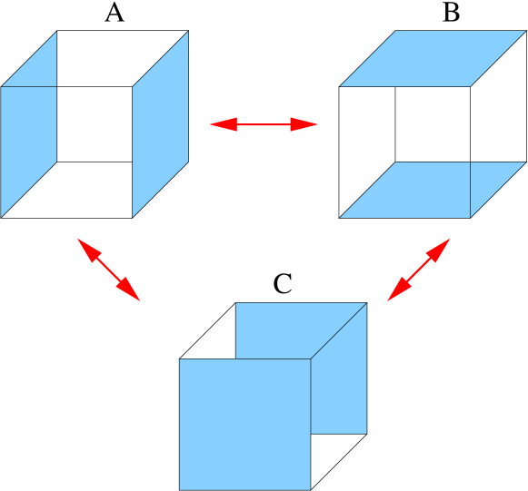
Figure 1: Three flippable configurations in one cube. The resonance is represented in the $t$-terim in Eq. 1.

The original RK Hamiltonian for quantum dimer model can be mapped to the compact $U(1)$ gauge theory Read and Sachdev (1990); Fradkin and Kivelson (1990), from which one can show that the 2+1 dimensional QDM is gapped except for one special RK point, while 3+1 dimensional QDM has a deconfined algebraic liquid phase Moessner and Sondhi (2003). By contrast, the quantum plaquette model in the cubic lattice can be mapped into a special type of lattice gauge field theory as follows. We denote all the square faces parallel to $XZ$ plane of the cubic lattice by the sites to the left and bottom corner of the face: $i+\frac{1}{2}\hat{x}+\frac{1}{2}\hat{z}$, and denote faces parallel to $XY$ and $YZ$ plane in a similar way. Then we define the boson number $n$ with integer values on every face of the cubic lattice. $n=1$ corresponds to a face with plaquette, and $n=0$ otherwise. A strong local potential term $U(n_{i+\frac{1}{2}\hat{\mu}+\frac{1}{2}\hat{\nu}}-\frac{1}{2})^{2}$ is turned on at every face to guarantee the low energy subspace of the boson Hilbert space is identical to the Hilbert space with all the plaquette configurations. Since every site is connected to one and only one plaquette, the summation of $n$ over all twelve faces sharing one sites needs to be $1$. Next, we define the rank-2 symmetric traceless tensor electric field on the lattice as

$$E_{i,\mu\nu}=\eta(i)(n_{i+\frac{1}{2}\hat{\mu}+\frac{1}{2}\hat{\nu}}-\frac{1}{2}),\ \ \ E_{\mu\nu}=E_{\nu\mu}(\mu\neq\nu),$$ (3)

where $\eta(i)=(-1)^{i_{x}+i_{y}+i_{z}}$ equals $1$ when $i$ belongs to one of the two sublattices of the cubic lattice and equals $-1$ otherwise. It is straightforward to check that the one-site-one-plaquette local constraint on the Hilbert space can be written compactly as

$$\nabla_{x}\nabla_{y}E_{xy}+\nabla_{y}\nabla_{z}E_{yz}+\nabla_{z}\nabla_{x}E_{zx}=5\eta(i),$$ (4)

where $\nabla$ is lattice derivative with the usual definition $\nabla_{\mu}f=f(i+\hat{\mu})-f(i)$.

The canonical conjugate variable of $E_{i,\mu\nu}$ is denoted as the vector potential of $A_{i,\mu\nu}$,

$$A_{i,\mu\nu}=\eta(i)\ \theta_{i+\frac{1}{2}\hat{\mu}+\frac{1}{2}\hat{\nu}},\ A_{\mu\nu}=A_{\nu\mu},\ (\mu\neq\nu).$$ (5)

$\theta_{i+\frac{1}{2}\hat{\mu}+\frac{1}{2}\hat{\nu}}$ is the canonical conjugate variable of boson number $n_{i+\frac{1}{2}\hat{\mu}+\frac{1}{2}\hat{\nu}}$, which is also the phase angle of boson creation operator. $A_{\mu\nu}$ and $E_{\mu\nu}$ satisfy

$$[E_{i,\mu\nu},A_{j,\rho\sigma}] = i\delta_{ij}(\delta_{\mu\rho}\delta_{\nu\sigma}+\delta_{\mu\sigma}\delta_{\nu\rho}).$$ (6)

Because $E_{\mu\nu}$ only takes values with an integer step, $A_{\mu\nu}$ is an compact field with period of $2\pi$. Due to the commutator

$$[E_{i,\mu\nu},\exp(iA_{j,\nu\sigma})]=(\delta_{\mu\rho}\delta_{\nu\sigma}+\delta_{\mu\sigma}\delta_{\nu\rho})\exp(iA_{j,\nu\sigma}),$$ (7)

operators $\exp(iA_{j,\nu\sigma})$ changes the eigenvalue of $E_{i,\mu\nu}$ by 1. As a result, the plaquette flipping process can be represented as

$$H_{t}= - t\big{\{}\cos(\nabla_{z}A_{xy}-\nabla_{x}A_{yz})$$

$$+ \cos(\nabla_{x}A_{yz}-\nabla_{y}A_{zx})$$

$$+ \cos(\nabla_{y}A_{zx}-\nabla_{z}A_{xy})\big{\}},$$ (9)

which is invariant under the gauge transformation of

$$A_{\mu\nu}\rightarrow A_{\mu\nu}+\nabla_{\mu}\nabla_{\nu}f,$$ (10)

which is already implied by the local constraint (4). $f$ is an arbitrary scalar function. The low energy Hamiltonian of the system can be written as

$$H = H_{t}+U\sum_{\mbox{each cube}}(E_{xy}^{2}+E_{yz}^{2}+E_{zx}^{2})$$

$$+ V\sum_{\mbox{each cube}}\Big{\{}(\nabla_{x}E_{yz})^{2}+(\nabla_{y}E_{zx})^{2}+(\nabla_{z}E_{zx})^{2}\Big{\}},$$

(11)

which is subject to the constraint in Eq. 4. Besides the gauge symmetry (10), Hamiltonian (11) together with constraint (4) share another symmetry as follows:

$$\mu\rightarrow-\mu,\ \rho\rightarrow\rho,\ \sigma\rightarrow\sigma,$$ (12)

$$E_{\mu\nu}\rightarrow-E_{\mu\nu},\ E_{\sigma\mu}\rightarrow-E_{\sigma\mu},\ E_{\nu\sigma}\rightarrow E_{\nu\sigma},$$ (13)

$$A_{\mu\nu}\rightarrow-A_{\mu\nu},\ A_{\sigma\mu}\rightarrow-A_{\sigma\mu},\ A_{\nu\sigma}\rightarrow A_{\nu\sigma}.$$ (14)

$\mu$, $\nu$ and $\sigma$ are three space coordinates. This symmetry forbids terms like $E_{xy}E_{yz}$ to be generated under RG flow at low energy.

III Duality transformation

A major question in which we are interested is whether the Hamiltonian Eq. 1 and Eq. 11 have an intrinsic liquid phase, just like the 3d QDM in the cubic lattice Moessner and Sondhi (2003). A liquid state here corresponds to a gapless Gaussian state in which we are allowed to expand the cosine functions in Eq. 11 at their minima, i.e., a “spin wave” treatment. However, the Gaussian phase could also be a superfluid phase which breaks the conservation of boson numbers (or effectively the plaquette numbers) with $\langle\exp(i\theta)\rangle\neq 0$. In our current problem a superfluid phase is not possible because $\langle\exp(i\theta)\rangle\neq 0$ necessarily breaks the local gauge symmetry (10) of Hamiltonian (11). In other words, a superfluid state is a coherent state of boson phase $\theta$ implying a strong fluctuation of boson numbers, which obviously violates the local one-site-one-plaquette constraint.

In this type of lattice bosonic models, because bosonic phase variable $A_{\mu\nu}$ is compact, the biggest obstacle of liquid phase is the proliferation of topological defect, which tunnels between two minima of the cosine function in Eq. 9. Since the topological defects are nonlocal, the best way to study them is go to the dual picture, in which the topological defects become local vertex operators of the dual height variables. similar duality transformations have been used widely in studying all types of bosonic rotor models, such as in proving the intrinsic gap of 2D QDM Fradkin and Kivelson (1990); Fradkin et al. (2004), showing the existence of “bose metal phase” Paramekanti et al. (2002) as well as the deconfine phase of 3d QDM Moessner and Sondhi (2003), and very recently the stable liquid phase of three dimensional “graviton” model Xu (2006).

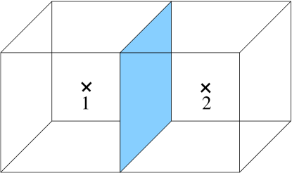
Figure 2: The duality transformation defined in Eq. 15. On dual site $1$ and $2$ there are three components of dual vector height $h_{\mu}$, and the dual transformation for the shaded face is $E_{yz}=(h_{y}-h_{z})_{2}-(h_{y}-h_{z})_{1}=\nabla_{x}(h_{y}-h_{z})$.

Besides the topological defects, another convenience one gains from the dual formalism is the solution of the constraint, i.e., we are no longer dealing with a Hilbert space with a strict one-site-one-plaquette constraint in Eq. 4. The dual variables are defined on the dual lattice sites $\bar{i}$, which are the centers of the unit cubes. In order to solve the constraint completely, one needs to introduce three components of the height field $h_{\mu}$ ($\mu=1$, 2, 3) on every dual site $\bar{i}$, which is the center of a unit cubic of the original lattice:

$$E_{xy} = \nabla_{z}(h_{x}-h_{y})+E_{xy}^{0},$$

$$E_{yz} = \nabla_{x}(h_{y}-h_{z})+E_{yz}^{0},$$

$$E_{zx} = \nabla_{y}(h_{z}-h_{x})+E_{zx}^{0},$$ (15)

whose geometric illustration is shown in Fig. 2. $h_{x,y,z}$ are fields only take discrete integer vaules. $E^{0}_{xy}$,$E^{0}_{yz}$ and $E^{0}_{zx}$ are background charges satisfying the constraint Eq. 4. We can just take the configuration of the columnar phase to define the value of the background charges as

$$E^{0}_{xy}(i,j,k) = \left\{\begin{array}[]{l}\frac{(-)^{k}}{2}\ \ \ (\mbox{when both i and j are even})\\ \frac{(-)^{i+j+k+1}}{2}\ \ \ (\mbox{otherwise})\end{array}\right.$$ (18)

$$E^{0}_{yz}(i,j,k) = E^{0}_{zx}(i,j,k)=\frac{(-)^{i+j+k+1}}{2}$$ (19)

The canonical momenta $\pi_{\mu}$ to the dual fields $h_{\mu}$ on each dual site are

$$\pi_{x} = \nabla_{y}A_{zx}-\nabla_{z}A_{xy},$$ (20)

$$\pi_{y} = \nabla_{z}A_{xy}-\nabla_{x}A_{yz},$$

$$\pi_{z} = \nabla_{x}A_{yz}-\nabla_{y}A_{zx}.$$ (21)

One can check the commutation relation and see that $\pi_{\mu}$ and $h_{\mu}$ are a pair of conjugate variables. Then the dual Hamiltonian of (11) reads

$$H = \sum_{\mu=x,y,z}-t\cos\pi_{\mu}+U\sum_{\mu\nu\rho}\zeta_{\mu\nu\rho}[\nabla_{\mu}(h_{\nu}-h_{\rho})-E^{0}_{\nu\rho}]^{2}$$ (22)

$$+ V\sum_{\mu\nu\rho}\zeta_{\mu\nu\rho}[\nabla_{\mu}(\nabla_{\mu}(h_{\nu}-h_{\rho})-E^{0}_{\nu\rho})]^{2}$$

$\zeta_{\mu\nu\rho}$ is a fully symmetric rank-3 tensor which equals zero when any two of its three coordinates equal, and equals one otherwise. On each dual lattice site $\bar{i}$, the $\pi_{\mu}$ fields satisfy the relation that $\sum_{\mu=x,y,z}\pi_{\mu,\bar{i}}=0$.

The symmetry transformations of Hamiltonian Eq. 22 can be extracted from the duality transformation Eq. 15 and Eq. 21:

$$h_{x}\rightarrow h_{x}+f(x,y,z)+g_{1}(x),$$ (23)

$$h_{y}\rightarrow h_{y}+f(x,y,z)+g_{2}(y),$$ (24)

$$h_{z}\rightarrow h_{z}+f(x,y,z)+g_{3}(z),$$ (25)

where $f$ is a function of three spatial coordinates and $g_{1,2,3}$ only depends on one spatial coordinate. This type of symmetry is a quasilocal symmetry, which also exists in the Bose metal states Paramekanti et al. (2002) and $p$-band cold atom systems Xu and Fisher (2007).

The main purpose of this paper is to study whether Hamiltonian (22) and (11) have a liquid phase which preserves all the lattice symmetries, just like the deconfined algebraic liquid phase of 3D QDM. In this kind of algebraic liquid phase, one can expand the cosine functions in equation (11) and relax the discrete values of the $h_{\mu}$ fields, the long distance physics can be described by a field theory which only involves coarsed grained mode of $h_{\mu}$, let us denote the long scale mode as $\tilde{h}_{\mu}$. In this Gaussian phase one can also define continuous tensor electric field $\tilde{E}_{\mu\nu}$ as the coarse grained mode of $E_{\mu\nu}$, the relation between $\tilde{E}_{\mu\nu}$ and $\tilde{h}_{\mu}$ is $\tilde{E}_{\mu\nu}=\zeta_{\mu\nu\rho}\partial_{\rho}(\tilde{h}_{\mu}-\tilde{h}_{\nu})$. A Gaussian field theory of $\tilde{h}_{\mu}$ should satisfy the continuous version of symmetries listed in Eq. 25 : $\tilde{h}_{\mu}\rightarrow\tilde{h}_{\mu}+\tilde{f}(x,y,z)+\tilde{g}_{\mu}(r_{\mu})$, now $\tilde{h}_{\mu}$ as well as functions $\tilde{f}$ and $\tilde{g}_{\mu}$ can all take continuous values. A low energy field theory action is conjectured to be

$$L=\sum_{\mu}\frac{K}{2}(\partial_{\tau}\tilde{h}_{\mu})^{2}+\frac{K}{2}\sum_{\mu\nu\rho}\zeta_{\mu\nu\rho}(\nabla_{\mu}(\tilde{h}_{\nu}-\tilde{h}_{\rho}))^{2}+\cdots,$$ (26)

where the $\tilde{h}_{x,y,z}$ fields take continuous real values. No other quadratic terms of $\tilde{h}_{\mu}$ with second spatial derivative is allowed by symmetry in this action. Notice that in Eq. 26 we have rescaled the space time coordinates to make the coefficients of the first and second term equal. The action (26) describes a state with enlarged conservation laws of $\pi_{\mu}$. If there is a state described by the Gaussian action (26), $\pi_{x}$, $\pi_{y}$ and $\pi_{z}$ are conserved within each $YZ$, $ZX$ and $XY$ plane respectively. So any operator with nonzero expectation values at this state has to satisfy the special 2d planar conservation law of $\pi_{\mu}$.

The Gaussian part of action (26) has one unphysical pure gauge mode which corresponds to function $f$ in Eq. 25, and two gapless physical modes, with low energy dispersion :

$$\omega^{2}_{1}\sim k_{x}^{2}+k_{y}^{2}+k_{z}^{2}+$$ (28)

(29)

$$\sqrt{k_{x}^{4}+k_{y}^{4}+k_{z}^{4}-k_{x}^{2}k_{y}^{2}-k_{y}^{2}k_{z}^{2}-k_{x}^{2}k_{z}^{2}},$$ (30)

(31)

$$\omega^{2}_{2}\sim k_{x}^{2}+k_{y}^{2}+k_{z}^{2}-$$ (32)

(33)

$$\sqrt{k_{x}^{4}+k_{y}^{4}+k_{z}^{4}-k_{x}^{2}k_{y}^{2}-k_{y}^{2}k_{z}^{2}-k_{x}^{2}k_{z}^{2}}.$$ (34)

The second mode $\omega_{2}$ vanishes at every coordinate axis of reciprocal space $(k_{x},k_{y},k_{z})$. The strong directional nature of $\omega_{2}$ roots directly in the quasilocal gauge symmetries in Eq. 25. The same modes can be obtained from the continuum Gaussian limit action of Hamiltonian (11):

$$L=\sum_{\mu\neq\nu}\frac{1}{2K}\{(\partial_{\tau}\tilde{A}_{\mu\nu})^{2}-\zeta_{\mu\nu\rho}(\partial_{\mu}\tilde{A}_{\nu\rho}-\partial_{\nu}\tilde{A}_{\rho\mu})^{2}\}.$$ (35)

In this action $\tilde{A}_{\mu\nu}$ is the coarse grained mode of $A_{\mu\nu}$, and $\tilde{A}_{\mu\nu}$ is no longer a compactified quantity. The fact that $\omega_{2}$ vanishes at every coordinate axis plays very important role in our following analysis, since it will create infrared divergence along each axis in the momentum space, instead of only at the origin. Similar directional modes are also found in other systems with quasilocal symmetries Paramekanti et al. (2002); Xu and Fisher (2007).

The ellipses in Eq. 26 contain the non-Gaussian vertex operators denoted as $L_{v}$, which manifests the discrete nature of $h_{\mu}$. Since $h_{\mu}$ only takes integer values, a periodic potential $\cos(2\pi h_{\mu})$ can be turned on in the dual lattice Hamiltonian (22). At low energy the Non-Gaussian term $L_{v}$ generated by $\cos(2\pi h_{\mu})$ has to satisfy all the symmetries in Eq. 25, the simplest form it can take is $\cos[2\pi\tilde{h}_{\mu}]$. However, this vertex operator only has lattice scale correlation at the Gaussian fixed point, because it violates the gauge symmetry of action (26). Thus the simplest vertex operator with possible long range correlation is

$$L_{v}=\sum_{\mu\neq\nu}-\alpha\cos[2\pi(\tilde{h}_{\mu}-\tilde{h}_{\nu})+\mathcal{B}_{\mu\nu}(\bar{i})].$$ (36)

and $\mathcal{B}(\bar{i})$ is a function of dual sites, which is interpreted as the Berry’s phase. The specific form of the Berry’s phase of the vertex operators depends on the background charge of the original gauge field formalism, which determines the crystalline pattern of the gapped phase Fradkin et al. (2004). However, since the liquid phase is a phase in which the vertex operators are irrelevant, whether a liquid phase exists or not does not depend on the Berry’s phase, thus in the current work we will not give a complete analysis of the Berry’s phase of our problem. In the continuum limit the most relevant vertex operators are the ones with multi-defects processes without Berry’s phase and consistent with symmetries (25): $\cos[2\pi N(\tilde{h}_{\mu}-\tilde{h}_{\nu})]$, let us denote this vertex operators as $V_{N,\mu\nu}$, and integer $N$ can be determined from detailed analysis of the Berry’s phase. The correlation function between two vertex operators with arbitrary $N$ separated in space time is calculated as follows:

$$\langle V_{N,\mu\nu}(0)V_{N,\mu\nu}(r)\rangle$$ (37)

(38)

$$\sim\exp\{-(2\pi)^{2}N^{2}\langle(\tilde{h}_{\mu}(0)-\tilde{h}_{\nu}(0))\ (\tilde{h}_{\mu}(r)-\tilde{h}_{\nu}(r))\rangle\}=$$ (39)

(40)

$$\delta_{r_{\mu}}\delta_{r_{\nu}}\exp\{-\frac{2(2\pi)^{2}N^{2}}{K}\int\frac{d^{4}k}{(2\pi)^{4}}\frac{(2k_{0}^{2}+3k_{\mu}^{2}+3k_{\nu}^{2})e^{i\vec{k}\cdot\vec{r}}}{(k^{2}_{0}+\omega_{1}^{2})(k^{2}_{0}+\omega_{2}^{2})}\}$$ (41)

(42)

(43)

$$\rightarrow\delta_{r_{\mu}}\delta_{r_{\nu}}\mathrm{Const}\ \ (r\rightarrow+\infty).$$ (44)

The correlation function $\langle\tilde{h}(r)\ \tilde{h}(r^{\prime})\rangle$ is evaluated at the Gaussian fixed point described by the continuum limit action (26) without $L_{v}$. The delta function $\delta_{r_{\mu}}\delta_{r_{\nu}}$ in Eq. 44 is due to the continuous quasilocal symmetry of action (26), or in other words the conservation of $\pi_{\mu}$ within each planes. For instance, correlation function $\langle e^{i2\pi N\{\tilde{h}_{x}(0)-\tilde{h}_{y}(0)\}}e^{-i2\pi N\{\tilde{h}_{x}(r)-\tilde{h}_{y}(r)\}}\rangle$ can only be nonzero when $r_{x}=r_{y}=0$, otherwise $\pi_{x}$ conservation within every $YZ$ plane will be violated once $r_{x}\neq 0$.

Since the correlation function calculated in Eq. 44 reaches a finite constant in the long distance limit, the vertex operators are very relevant at the Gaussian fixed point described by the action Eq. 26, and the system is generally gapped with crystalline order in the whole phase diagram. Since this result is applicable to any $N$ and independent of the Berry’s phase, the same conclusion is applicable to all the QPM with a definite number of plaquette connected to each site. The specific crystalline order can be determined from the detailed analysis of the Berry’s phase.

IV Classical RK point

At the RK point, the ground state wave-function is an equal weight superposition of all the configurations allowed by constraint (4). All the static physics of this state is mathematically equivalent to a classical ensemble, with partition function defined as summation of all the plaquette configurations with equal Boltzman weights. Since there is no energetic terms in the partition function, all that rules is the entropy. If we define the tensor electric field as Eq. 3, the classical ensemble can be written as

$$Z=\sum_{E_{i,\mu\nu}}\delta\{\sum_{\mu\neq\nu}\ \nabla_{\mu}\nabla_{\nu}E_{\mu\nu}-5\eta(i)\}$$ (45)

$$\times\exp\{-U\sum_{i}\sum_{\mu\neq\nu}(E_{i,\mu\nu})^{2}\}.$$ (46)

The delta function enforces the constraint, and the term $-U\sum_{\mu\neq\nu}(E_{i,\mu\nu})^{2}$ in the exponential makes sure all the low energy $E_{\mu\nu}$ configurations are one-to-one mapping of the plaquette configurations. Now solving the constraint by introducing dual height field $h_{\mu}$, the classical partition function can be rewritten as

$$Z=\sum_{h_{\bar{i},\mu}}\exp\{-U\sum_{\bar{i}}\sum_{\mu\nu\rho}\zeta_{\mu\nu\rho}[\nabla_{\mu}(h_{\bar{i},\nu}-h_{\bar{i},\rho})-E^{0}_{\nu\rho}]^{2}\}.$$ (47)

Again we are mainly interested in whether this classical ensemble is an algebraic liquid state, or by tuning parameters one can reach an algebraic liquid phase. We can conjecture a low energy classical field theory generated by entropy, allowed by symmetry (25). The same strategy has been used to study classical six-vertex model, classical three-color model and four color model J.Kondev and C.L.Henley (1996). Here the simplest low energy effective classical field theory reads

$$F=\sum_{\mu\nu\rho}\frac{\tilde{K}}{2}\zeta_{\mu\nu\rho}(\nabla_{\mu}(\tilde{h}_{\nu}-\tilde{h}_{\rho}))^{2}+\cdots.$$ (48)

The number $\tilde{K}$ cannot be determined from our field theory. This is the simplest free energy allowed by symmetry. The physical meaning of this free energy is that, the total number of plaquette configurations (entropy) in a three dimension volume is larger if the average tensor electric field $E_{\mu\nu}$ is small, i.e. the entropy favors zero average tensor electric field.

The ellipses in equation (48) includes the vertex operators in equation (36). The relevance of the vertex operators can be checked by calculating the scaling dimensions of the vertex operators at the Gaussian fixed point action (48). Let us denote vertex operator $\cos[2\pi N(\tilde{h}_{\mu}-\tilde{h}_{\nu})]$ as $V_{N,\mu\nu}$. Due to the symmetry (25), $V_{N,xy}$ can only correlates with itself along the same $\hat{z}$ axis, and $V_{N,zx}$ and $V_{N,yz}$ can never have nonzero correlation between each other when they are separated spatially along $\hat{z}$ axis.

The leading order correlation functions are

$$\langle V_{N,xy,(0,0,0)}V_{N,xy,(0,0,z)}\rangle$$ (49)

(50)

$$\sim\exp\{-\frac{(2\pi)^{2}N^{2}2}{\tilde{K}}\int\frac{d^{3}k}{(2\pi)^{3}}\frac{(k_{x}^{2}+k_{y}^{2})e^{ik_{z}z}}{k_{x}^{2}k_{y}^{2}+k_{y}^{2}k_{z}^{2}+k_{z}^{2}k_{x}^{2}}\}$$ (51)

(52)

$$=\frac{1}{z^{8\pi N^{2}/\tilde{K}}}.$$ (53)

In the above calculations we have chosen the simplest regularization: replacing spatial derivative on the lattice by momentum $ik_{x}$. It has been shown that the scaling dimensions of operators in these type of models with extreme anisotropy can depend on the regularization on the lattice Paramekanti et al. (2002). Here the scaling dimension of operator $V_{N,\mu\nu}$ is regularization independent. These vertex operators are irrelevant if $\tilde{K}<\tilde{K}_{c}=4\pi N^{2}$, in this parameter regime the contribution of $V_{N,xy}$ to various correlation functions can be calculated perturbatively.

Some other vertex operators can be generated under renormalization group flow, but these vertex operators all have algebraic correlations, with a regularization dependent scaling dimension proportional to $1/\tilde{K}$. For instance, vertex operator $\cos[2\pi N\nabla^{n}_{mx}(\tilde{h}_{x}-\tilde{h}_{y})]$ has nonzero algebraic correlation function in the $YZ$ plane at long distance. Here lattice derivative $\nabla_{mx}$ is defined as $\nabla_{mx}f(\vec{r})=f(\vec{r}+m\hat{x})-f(\vec{r})$. If we regularize the theory by replacing lattice derivative $\nabla_{mx}$ with $i2\sin(mk_{x}/2)$ in the momentum space, the scaling dimension of $V_{N,mx,xy}=\cos[2\pi N\nabla^{n}_{mx}(\tilde{h}_{x}-\tilde{h}_{y})]$ with $n=1$ and arbitrary integer $m$ is $4\pi N^{2}/\tilde{K}$, and the scaling dimension is isotropic in the whole $YZ$ plane:

$$\langle V_{N,mx,xy,(0,0,0)}V_{N,mx,xy,(0,y,z)}\rangle\sim\frac{c(\theta)}{(y^{2}+z^{2})^{4\pi N^{2}/\tilde{K}}}.$$ (54)

Here $c(\theta)$ is a positive function of $\theta=\arctan(z/y)$. Notice that the rotation symmetry in the $YZ$ plane is not restored even at long length scale. The scaling dimension of $\cos[2\pi N\nabla^{n}_{mx}(\tilde{h}_{x}-\tilde{h}_{y})]$ increases rapidly with number $n$. Thus all the vertex operators are irrelevant when $\tilde{K}$ is small enough, and there is a critical $\tilde{K}_{c}$ separating a crystalline order and the algebraic liquid phase. At the liquid line the crystalline order parameter should have algebraic correlation functions. Coefficient $\tilde{K}$ can be tuned from adding energetic terms in the system. Recall that now the configurations with zero average $E_{\mu\nu}$ are favored by entropy, if we want to reduce $\tilde{K}$, we can add energetic terms which disfavor zero average $E_{\mu\nu}$. For instance, if we give the flippable cubics a smaller weight than the unflippable cubics, coefficient $\tilde{K}$ should be reduced.

The above results can be roughly understood from simple physical argument. Notice that all the flippable cubes have zero average electric field, so the entropy effectively favors flippable cubes. If $\tilde{K}>\tilde{K}_{c}$, the entropy strongly favors flippable cubes, the system will develop crystalline order which maximize the number of flippable cubes. This kind of effect is usually called “order by disorder”. It is also natural that the crystalline order tends to be weakened or even melt if we reduce $K$. Since the melting transition of the crystalline order is driven by the proliferation of defect operators, the universality class of this transition is very similar to the Kosterlitz-Thouless transition of the 2D XY model, the correlation length between operators $V_{N,\mu\nu}$ diverges as $\xi\sim\exp[\sqrt{b/(\tilde{K}-\tilde{K}_{c})}]$. Unusual KT like transition in 3d or higher dimensions have also been discussed in other systems with similar quasilocal symmetries Paramekanti et al. (2002), where the dimensionality of the system is effectively reduced to 2d.

Recent Monte Carlo simulation Pankov et al. (2007) shows that the whole phase diagram of RK Hamiltonian (1) is gapped with crystalline order, including the RK point. Our results based on duality is consistent with this numerical results, and the equal weight classical partition function should have $\tilde{K}>\tilde{K}_{c}$. Our theory also predicts that if we turn on energetic terms which favors unflippable cubes, there is a critical line described by Gaussian field theory (48). This prediction can be checked by classical Monte Carlo simulations. Another prediction which in principle can be made in our formalism is the most favored crystalline order when $\tilde{K}$ is slightly larger than $\tilde{K}_{c}$. This requires a detailed analysis of the Berry’s phase of the vertex operators in the dual theory, which we leave to future studies.

V topological sector

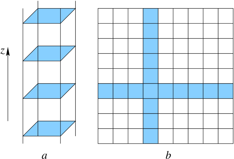
Figure 3: ($a$), the conserved quantity $m_{xy}$ is defined as the summation of all $E_{xy}$ on all the shaded squares along one $z$ axis. ($b$), the view of the 3d lattice from the top. If the quantity $m_{xy}$ is fixed on all the shaded squares shown in this figure, $m_{xy}$ is determined on the whole lattice.

Now let us discuss the topological sector, within which every configuration can be connected to each other through finite local movings depicted in Fig. 1. Topological sectors are especially useful when one is dealing with a quantum liquid state, where Landau’s classification of phases are no longer applicable. In the original quantum dimer model on square lattice, the topological sector on a torus is specified by two integers Rokhsar and Kivelson (1988), which can be interpreted as winding numbers of electric fields. Here we choose a lattice with even number of sites in each axis and impose the periodic boundary condition. To specify a topological sector one needs to know the conserved quantities under local movings. It is straightforward to check that quantity $m_{i_{x},i_{y},xy}=\sum_{i_{z}}E_{i,xy}$ for any 2d coordinate $(i_{x},i_{y})$ is a conserved quantity. Notation $\sum_{i_{z}}$ means summation over all the sites with the same $x$ and $y$ coordinates (Fig. 3). However, these quantities are not independent. For instance, using constraint (4) we have the following identity:

$$m_{0,0,xy} - m_{1,0,xy}+m_{1,1,xy}-m_{0,1,xy}=\sum_{i_{z}}\nabla_{x}\nabla_{y}E_{xy}$$ (55)

$$= \sum_{i_{z}}5\eta(i)-(\nabla_{y}\nabla_{z}E_{yz}+\nabla_{z}\nabla_{x}E_{zx})=0.$$ (57)

Thus as long as one fix the quantity $m_{xy}$ for one column and one row in the $XY$ plane, their values for the whole lattice are determined. Conserved quantities associated with $E_{zx}$ and $E_{yz}$ can be treated in the same way. Thus we conclude that one needs infinite number of integers to specify a topological sector on a three dimension torus, and the number scales with the linear size of the lattice.

VI Summary and comparison with other models

This work studies a three dimensional quantum resonating plaquette model, motivated from a special SU(4) invariant point in spin-3/2 cold atom system. The effective low energy physics of the problem can be mapped to a special type of lattice gauge field. Our current QPM together with previously studied 3d QDM Moessner and Sondhi (2003) and soft-graviton model Xu (2006) all have local constraint and low energy gauge field description without gapless matter fields. Unlike the QDM and the soft-graviton model, the QPM almost always suffers from the proliferation of topological defects, and a generic stable algebraic liquid state as an analogue of the photon phase of 3d QDM does not exist.

The reason of the existence of a stable liquid phase of 3d QDM as well as the 3d soft-graviton model have been discussed in reference Xu (2006). Both models with stable liquid phases are self-dual gauge theories, with strong enough gauge symmetries in both the original description of the problem or the dual theories, i.e. one cannot write down a gauge invariant vertex operator which gaps out the liquid phase. In our current QPM, the symmetry of the dual theory does not rule out all the vertex operators, and gauge invariant vertex operators are very relevant. Thus in this type of bosonic quantum rotor models, large enough gauge symmetries are necessary for both sides of the duality to guarantee the existence of a stable liquid phase if gapless matter field is absent.