Comparative Analysis of Control Strategies

Abstract

Different ways of modelling quantum control systems, formulating control problems and solving the resulting problems are considered and compared. In particular, we compare the performance of geometric and optimal control, as well as iterative techniques for optimal control design versus local gradient optimization using a Lyapunov-type potential function for two problems of general interest: global control of qubits and entanglement generation in the form of Bell state preparation.

I Introduction

Motivated in part by the rapid growth of nanofabrication techniques and nanotechnology, as well as a surge of interest in novel applications of quantum effects such as quantum information processing, the control of quantum systems is a subject that has received considerable attention recently. Many control strategies for quantum systems have been proposed, from open-loop strategies for Hamiltonian engineering involving usually off-line design of control fields based on a model of the system, assuming knowledge of the initial state and the control objective, to closed-loop strategies mostly based on conditional quantum trajectories and continuous weak measurements [1]. Some variants of open-loop Hamiltonian engineering have enjoyed considerable success in various experimental settings [2, 3] in the form of adaptive open-loop techniques such as direct laboratory optimization [4, 5]. However, despite the obvious practical importance of selecting the best strategy, very little work has been done in comparing different control strategies in terms of their effectiveness, efficiency and robustness. This is the topic of this paper. We will restrict ourselves here to comparing open-loop control strategies, and focus specifically on geometric, Lyapunov and iterative optimal control design techniques.

There are many ways of formulating problems in quantum control as optimal control problems, from time-optimal control [6] to variational techniques [7, 8, 9, 10] incorporating various constraints, e.g., on pulse energies, amplitudes and frequencies. In addition, many quantum control problems can be formulated either as state control problems (using either a pure state vector, wave-function, density operator or real coherence vector representation), as optimization of observables problems, or as process control problems (e.g. producing a desired quantum logic gate). Unfortunately, although these mathematical models are often equally valid, if not equivalent, ways of describing the system and control objective, we find that different formulations of the problem can lead to different solutions for the optimal control field. This is significant, as the solutions are not always equally desirable from a practical or physical point of view. Different formulations have different complexities when it comes to solving the resulting equations, either numerically or analytically.

Finally, once a particular model and problem formulation have been chosen, there are various ways of solving the resulting control problem, ranging from direct single-step control design methods based on Lyapunov potential functions [11, 12], to iterative techniques for control field design using gradient-based optimization algorithms such as GRAPE [10] and other monotonically convergent algorithms [7, 8, 9]. Unfortunately, again, even if the formulation of the control problem is the same, different techniques can yield very different solutions. The choice of algorithm for a particular control problem may depend on further factors. Certain algorithms are more flexible, allowing more realistic models to be used, such as the inclusion of non-Hamiltonian processes or a realistic restriction on the capabilities of the pulse-shaping equipment. Other algorithms are numerically and computationally far simpler—finding a global optimal solution is simpler for geometric control (where it is equivalent to finding a geodesic, and has an analytic solution for many systems) than for an optimal control problem (where the numerical solution and discretization of the solution is non-trivial to globally optimize). The techniques also have different degrees of robustness to errors in our models of the systems. These competing issues of numerical accuracy, facility of implementation and robustness to modelling and systematic error must be appreciated to find the best practical solution.

Since we obviously cannot address all of these problems in a single paper, we will illustrate some of the issues considering two typical problems of significance in quantum computing scenarios: simultaneous, selective control of several qubits using global control pulses, and controlled entanglement of coupled qubits. We will compare geometric and optimal control design, based on direct optimization of a Lyapunov function and iterative optimal control design using monotonically convergent algorithms. Before we delve into comparing different control design techniques in Sections IV and V, we briefly consider different ways of modelling quantum control systems and formulating quantum control problems in Sec II, and review the relevant control design techniques in Sec. III.

II Modelling quantum control systems & control problems

As eluded to in the introduction, quantum systems can be modelled in various ways. Systems initially in a pure state, i.e., unentangled with their environment and governed by Hamiltonian evolution can be described by a wavefunction encoding information about the state of the system that evolves according to a control-dependent Schrodinger equation

$$i\hbar|\Psi({\bf x},t)\rangle=H[{\bf x},{\bf f}(t)]|\Psi({\bf x},t)\rangle$$ (1)

where $H[{\bf x},{\bf f}(t)]$ is the control-dependent Hamiltonian and ${\bf f}$ the control field applied. For convenience we will choose units here so that $\hbar=1$. In general, the wavefunction of the system is a normalizable and differentiable complex-valued function of time $t$ and space ${\bf x}$, and $\hat{H}$ is a partial differential operator, but Eq. (1) can be recast as an ordinary differential equation, e.g., by expanding $|\Psi({\bf x},t)\rangle$ in terms of the eigenstates $|n\rangle$ of $\hat{H}_{0}$, the system’s intrinsic Hamiltonian, $|\Psi({\bf x},t)\rangle=\sum_{n=1}^{N}c_{n}|n\rangle$, where $N$ is the dimension of the Hilbert space $\mathcal{H}$, in which case we simply obtain a linear matrix ODE

$$\dot{{\bf c}}(t)=-i\hat{H}[{\bf f}(t)]{\bf c}(t),$$ (2)

where ${\bf c}$ is a complex column vector, usually normalized to unity, $\|{\bf c}\|=1$, and $\hat{H}[{\bf f}(t)]$ is simply a control-dependent $N\times N$ Hermitian matrix. The dependence of the Hamiltonian on the control fields is furthermore often assumed to be linear so that

$$\hat{H}[{\bf f}(t)]=\hat{H}_{0}+\sum_{m=1}^{M}f_{m}(t)\hat{H}_{m},\quad M<\infty.$$ (3)

This the standard model for pure-state quantum control.

We can also represent the state of the system by an operator $\hat{\rho}(t)$ acting on the Hilbert space $\mathcal{H}$. For a pure-state system represented by $|\Psi({\bf x},t)\rangle\equiv{\bf c}(t)$, we have simply $\hat{\rho}(t)=|\Psi({\bf x},t)\rangle\langle\Psi({\bf x},t)|\equiv{\bf c}{\bf c}^{\dagger}$, where ${\bf c}^{\dagger}$ is the Hermitian conjugate of ${\bf c}$, from which we can immediately deduce the evolution equation

$$\dot{\hat{\rho}}(t)=-i\left[\hat{H}[{\bf f}(t)],\hat{\rho}(t)\right],$$ (4)

where $[A,B]=AB-BA$ is the matrix commutator. For a pure-state system subject to Hamiltonian evolution the latter formulation is equivalent to Eq. (2). Its main advantage is that it can be extended to systems initially entangled with their environment, i.e., in a non-pure quantum state, or can interact (non-coherently) with their environment by adding a non-Hermitian super-operator ${\text{\liouvop L}}_{D}[\hat{\rho}(t)]$ to the RHS of Eq. (4).

Finally, we can represent the state of a quantum system in terms of the (real) expectation values of a complete set of (Hermitian) observables. There are obviously many choices for the set of observables but a very convenient choice are the normalized Pauli matrices

$$\hat{\sigma}_{rs}^{x} = \frac{1}{\sqrt{2}}(|r\rangle\langle s|+|s\rangle\langle r|)$$

$$\hat{\sigma}_{rs}^{y} = \frac{i}{\sqrt{2}}(-|r\rangle\langle s|+|s\rangle\langle r|)$$

$$\hat{\sigma}_{r}^{z} = \sqrt{\frac{1}{r+r^{2}}}\left(\sum_{k=1}^{r}|k\rangle\langle k|-r|r+1\rangle\langle r+1|\right)$$

for $1\leq r\leq N-1$ and $r<s\leq N$. It is easy to show that the $N^{2}-1$ trace-zero matrices $\hat{\sigma}_{k}$ above, together with the normalized identity operator $\hat{\sigma}_{0}=\frac{1}{\sqrt{N}}\hat{I}$, form a complete orthonormal basis for the Hermitian operators on $\mathcal{H}$, and hence we have $\hat{\rho}=\sum_{n=0}^{N^{2}-1}s_{n}\hat{\sigma}_{k}$ with $s_{k}=\langle\hat{\sigma}_{k}\mid\hat{\rho}\rangle=\operatorname{Tr}(\hat{\sigma}_{k}^{\dagger}\hat{\rho})$. Thus, we can represent any quantum state $\hat{\rho}$ by a real $N^{2}-1$ vector ${\bf s}=(s_{k})_{k=1}^{N^{2}-1}$, where $s_{0}=1/\sqrt{N}$ is omitted as it is constant. The vector ${\bf s}$ is generally called the Bloch or coherence vector in the physical literature, or the Stokes tensor in the mathematical literature. This Bloch representation is very popular especially for two-level systems as it permits visualization of quantum states as points inside a ball in $\mathbb{R}^{3}$.  It is very easy to see that Eq. (4) thus gives rise to the so-called Bloch equation

$$\dot{{\bf s}}(t)=A[{\bf f}(t)]{\bf s}(t),$$ (5)

and Eq. (3) implies $A=A_{0}+\sum_{m=1}^{M}f(t)A_{m}$, where $A_{m}$ are real-orthogonal matrices given by $A_{m}=\mbox{ad}_{\hat{H}_{m}}$ for $m=0,\ldots,M$, for Hamiltonian systems. For dissipative systems one can derive an affine-linear Bloch equation $\dot{{\bf s}}(t)=A[{\bf f}(t)]{\bf s}(t)+{\bf b}$, although we shall not discuss this case here.

As this brief overview shows, there are several ways of modelling quantum systems, which are often equally valid or even mathematically equivalent descriptions of the system. We shall see, however, that they are not necessarily equally desirable from a practical point of view, and depending on the problem considered, some may in fact be highly preferable to others.

But even if we have chosen a particular way to model the system, most quantum control problems can be formulated in many different ways. For instance, the three ‘canonical’ control problems

• State control: Steer the system from a given initial state to a desired target state

• Process control: Implement a desired quantum process (unitary operator for Hamiltonian systems)

• Observable control: Drive the system such as to optimize the expectation value of an observable

are inter-convertible. E.g., a pure state control problem can be formulated as observable optimization problem where the observable is the projector onto the desired pure state. A mixed-state control problem can be formulated as an observable optimization problem with $\hat{A}=\hat{\rho}$. An observable optimization problem can be translated into the problem of simultaneously driving a set of basis states to coincide with the desired eigenstates of the observable, etc. In addition to many obvious choices, there are often less obvious ones that may turn out to be easier to solve than the more obvious choices.

III Control design techniques for quantum systems

Before we compare control design techniques, we briefly review the relevant techniques. The simplest control design strategy, with a long history of successful application in nuclear magnetic resonance experiments, is the use of geometric control pulse sequences. Although it is rarely formulated this way in NMR spectroscopy, the basic idea of geometric control is to find a target (unitary) operator that will achieve the control objective—be that the implementation of a particular process, or the preparation of a quantum state, etc—and to decompose or factorize it, using standard techniques such as the generalized Euler angle or Cartan decomposition, into elementary operations that can be practically realized by applying simple geometric control pulses such as piecewise constant controls or Gaussian pulses, for example. Typically, geometric control sequences can be visualized as performing a sequence of rotations on Bloch vectors in $\mathbb{R}^{N^{2}-1}$, whence the name geometric control.

An alternative to simple geometric pulse sequences is the use of temporally or spectrally shaped pulses optimized for a particular task. The design of optimally shaped pulses is a non-trivial problem, which is usually solved numerically using one of a number of (similar) iterative techniques [7, 8, 9, 10]. The particular algorithm we will employ in the following involves iteratively solving an initial value problem for a variational trial function $S_{v}^{(n)}(t)$ representing the state of the system

$$\dot{S}_{v}^{(n)}(t)={\text{\liouvop L}}[{\bf f}^{(n)}(t),S_{v}^{(n)}(t)],\qquad S_{v}^{(n)}(t_{0})=S_{0},$$ (6)

followed by a final value problem for a variational trial function $A_{v}^{(n)}(t)$ (usually representing an observable)

$$\dot{A}_{v}^{(n)}(t)={\text{\liouvop L}}[{\bf f}^{n}(t),A_{v}^{(n)}(t)],\qquad A_{v}^{(n)}(t_{F})=A_{F},$$ (7)

while updating the control field in each step according to

$$f^{(n)}_{m}(t) = (1-\alpha)\tilde{f}_{m}^{(n-1)}-\frac{i\alpha}{\lambda}\frac{\delta\mathcal{J}(A_{v}^{(n-1)},S_{v}^{(n)},f_{m}^{(n)})}{\delta f_{m}}$$

$$\tilde{f}_{m}^{(n)}(t) = (1-\beta)f_{m}^{(n)}-\frac{i\beta}{\lambda}\frac{\delta\mathcal{J}(A_{v}^{(n)},S_{v}^{(n)},f_{m}^{(n)})}{\delta f_{m}}$$

starting with an initial trial field ${\bf f}^{(0)}(t)$, and setting

$$\frac{\delta\mathcal{J}(A_{v},S_{v},f_{m})}{\delta f_{m}}\equiv\langle A_{v}(t)\mid\partial_{f_{m}(t)}{\text{\liouvop L}}[{\bf f}(t),S_{v}(t)]\rangle.$$ (8)

In the abstract notation above, $S_{v}$ could be a pure state $|\Psi_{v}\rangle$, a density matrix $\hat{\rho}_{v}$, a real Bloch vector ${\bf s}_{v}$, or even a unitary operator $\hat{U}_{v}$; $A_{v}$ is a suitable conjugate variable. The super-operator ${\text{\liouvop L}}[{\bf f}(t),S_{v}(t)]$ depends on the chosen model. For a Hamiltonian pure-state system

$${\text{\liouvop L}}[{\bf f}(t),S_{v}(t)]\equiv-i\hat{H}[{\bf f}(t)]|\Psi_{v}(t)\rangle,$$

for a general mixed-state system

$${\text{\liouvop L}}[{\bf f}(t),S_{v}(t)]\equiv-i\left[\hat{H}[{\bf f}(t)],\hat{\rho}_{v}(t)\right]+{\text{\liouvop L}}_{D}[\hat{\rho}_{v}(t)],$$

and for a unitary operator control problem $-i\hat{H}[{\bf f}(t)]\hat{U}_{v}(t)$, etc. For a system with control-linear Hamiltonian (3) the derivatives of the dynamic operator with respect to $f_{m}(t)$ are explicitly

$$\langle A_{v}(t)\mid\partial_{f_{m}}{\text{\liouvop L}}[{\bf f}(t),S_{v}(t)]\rangle\equiv\langle\chi_{v}(t)|\hat{H}_{m}|\Psi_{v}(t)\rangle$$ (9)

for a pure-state system,

$$\langle A_{v}(t)\mid\partial_{f_{m}}{\text{\liouvop L}}[{\bf f}(t),S_{v}(t)]\rangle\equiv\operatorname{Tr}\left(A_{v}(t)[\hat{H}_{m},\rho_{v}(t)]\right),$$ (10)

for a mixed-state system, etc. $\alpha$, $\beta$, $\lambda$ and the target time $t_{F}$ are non-negative real parameters with $0\leq\alpha,\beta<2$ to ensure convergence. It is possible to let $\alpha$, $\beta$ and $\lambda$ be positive functions rather than constants but we shall assume constant values in this paper.

The third technique we consider is model-based (open-loop) control design using Lyapunov functions. This approach essentially involves choosing the control field at every point in time such as to ensure the dynamical evolution results in the monotonic decrease of a Lyapunov potential $V$, which has a minimum at our target state. If the objective is to reach a given target state, an obvious choice for $V$ is a monotonic function of the distance between the current and target states of the system, e.g., $V(\rho,\rho_{d})=\|\rho-\rho_{d}\|^{2}$, if we use the density operator formulation, $V(\psi,\psi_{d})=\|\psi-\psi_{d}\|^{2}$ in the pure state formulation, or $V({\bf s},{\bf s}_{d})=\|{\bf s}-{\bf s}_{d}\|^{2}$ if we use the Bloch vector representation of the state. Regardless of the precise formulation, one easily obtains a simple rule for choosing the control field. For instance, in the Bloch representation, given a system satisfying $\dot{{\bf s}}(t)=A[f(t)]{\bf s}(t)$ with $A[f(t)]=A_{0}+f(t)A_{1}$ where $A_{0}$ and $A_{1}$ are dynamical generators, we can easily obtain the rule $f(t)=\kappa{\bf s}_{d}(t)^{T}A_{1}{\bf s}(t)$, where $\kappa$ is a positive constant. The obvious advantage of this approach is that we obtain an explicit control law, and under certain conditions, asymptotic convergence from a near-global set of target states to the target state can be proved [11, 12].

IV Geometric vs optimal control

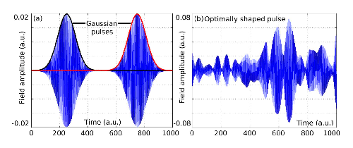
Figure 1: (a) Two Gaussian wave-packets with ‘pulse area $\pi$’ with frequencies $\omega_{1}$ (pulse 1, black envelope) and $\omega_{3}$ (pulse 2, red envelope), respectively. (b) Optimally shaped pulse to achieve simultaneous selective excitation of dots $1$ and $3$ while minimizing the (final) excitation of all other dots.

As an explicit problem in this section we consider an ensemble of five quantum dots, which will be modelled as a two-level systems (qubits) with slightly different energy levels. Obviously, this is a simplification. Real systems will have more energy levels but it is a good model system to study the limitations of frequency selective geometric control and explore what improvements might be gained using optimally shaped pulses. The control objective is simultaneous, selective control of all qubits using global control pulses, i.e., the ability to simultaneously perform selective gate operations on several qubits without any local addressing. For the first example we consider local operations and assume negligible inter-qubit coupling on the time-scales relevant for single qubit gates.

If the individual qubits have different resonance frequencies, due to variations in size, shape or composition of the dots (as fabricated systems such as quantum dots usually do), the simplest control approach is to employ frequency-selective geometric control pulses to selectively induce desired single-qubit rotations without local addressing. This approach is attractive due to its simplicity, and frequency-selective geometric control pulse sequences have been used successfully in nuclear magnetic resonance (NMR) applications, and to a lesser extent in electron spin resonance experiments. However, in practice such simple control pulse sequences are generally not optimal (for gate operation times and other figures of merit), and problems are expected to arise, e.g., when the frequency separation between the individual qubits is small, and fast control operation is desired to minimize gate operation times and deleterious effects of decoherence. In this case, we expect optimal control designs to out-perform the simple geometric schemes. Indeed, simulations show that this is generally the case.

To consider a concrete example, we compare the Bloch trajectories for a simple geometric pulse sequence and an optimally shaped pulse for the problem of performing simultaneous bit flips on two qubits (here $1$ and $3$) without affecting the others. (The bit flip operation was chosen as it is easy to visualize on the Bloch sphere. Similar results hold for other single qubit gates.) The geometric control solution in this case is simple: apply a sequence of two $\pi$ pulses resonant with the transition frequencies of the two target dots. If the control pulses are sufficiently long, the geometric control pulse sequence produces very good results. However, as we reduce the pulse lengths and increase the pulse strengths, off-resonant excitation becomes a problem, as Fig. 1 shows. The left column (a) shows the ideal evolution of each dot in the rotating frame subject to the fields in Fig 1 (a). Target dots $1$ and $3$ follow a smooth path from south to north pole, the others are unaffected. However, the middle column (b), which shows the actual evolution of the quantum dots in the stationary lab frame when subjected to the control fields in Fig 1 (a), shows clearly that the applied pulses induce far more complex evolution. Dots $1$ and $3$ are resonantly excited, leading to population transfer from the south to the north pole along a spiral path in the stationary frame, as desired. However, there is also significant off-resonant excitation of the remaining dots, all of which are left in various excited states at the final time. The right column (c) shows the path of the dots subject to field 1 (b): despite following complicated trajectories both target dots finish at the north pole and all the other dots are returned to the south pole (ground state) at the final time, leaving no unwanted excitations.

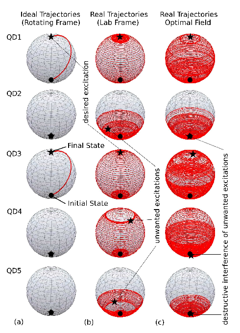
Figure 2: Bloch sphere trajectories for five quantum dots (with resonance frequencies of $1.32$, $1.35$, $1.375$, $1.38$, $1.397$ eV, respectively) subject to two Gaussian pi pulses of approximately 2 pico-seconds each (a,b), and a shaped pulse designed using iterative optimal control (c). The actual trajectories for the geometric control pulse sequence (b) differ significantly from the ideal model trajectories (a).

The optimal pulse shown in Fig 1 (b) was designed by formulating the problem as an optimization problem for the observable $\hat{A}=\operatorname{diag}(0,1,0,-1,0,1,0,-1,0,-1)$, defined on the Hilbert space $\mathcal{H}=\oplus_{k=1}^{5}\mathcal{H}_{k}$, where $\mathcal{H}_{k}$ is the single qubit Hilbert space. Although for five qubits the problem of directly optimizing the average gate fidelity on the 32-dimensional direct product space $\otimes_{k=1}^{5}\mathcal{H}_{k}$ is computationally still tractable on modern computers, our rather unintuitive formulation was considerably more efficient here. Since we assumed inter-dot coupling to be negligible for pico-second pulses in our example, it is sufficient to model the evolution of the individual dots (for the purpose of implementing single qubit gates) on the direct sum Hilbert space $\mathcal{H}=\oplus_{k=1}^{5}\mathcal{H}_{k}$, which has only dimension $10$. Furthermore, the observable $\hat{A}$ here assumes its maximum exactly when dots $1$ and $3$ are in the excited state $|1\rangle$ and all others are in the ground state $|0\rangle$. Since all our dots are initially in the ground state $|0\rangle$, optimizing $\langle A\rangle$ requires implementing a unitary operator $\hat{U}$ such that $\hat{U}|0\rangle_{k}=|1\rangle_{k}$ for $k=1,3$ and $\hat{U}|0\rangle_{k}=|0\rangle_{k}$ for $k=2,4,5$. For this simple example it is easy to see that the only unitary operator (in $\oplus_{k=1}^{5}\mathfrak{SU}(2)$) that achieves this (on the direct sum Hilbert space) is indeed $\hat{U}=\hat{X}\oplus\hat{I}\oplus\hat{X}\oplus\hat{I}\oplus\hat{I}$ where $X=\begin{pmatrix}0&1\\ 1&0\end{pmatrix}$ is the bit flip operator—the operator we wanted to implement. Similar observables can be constructed to implement simultaneous local operations on $N$ uncoupled qubits, although the approach does not straightforwardly generalize to qudit systems.

The optimal control problem thus defined was solved using the iterative optimal control design algorithm described in Sec. III. The Liouville operator for the system under consideration was

$${\text{\liouvop L}}[f(t),\rho(t)]=[\hat{H}_{0}+f(t)\hat{H}_{1},\hat{\rho}(t)],$$ (11)

where $\hat{H}_{m}=\operatorname{diag}(H_{m}^{(k)})$, $k=1,\ldots,5$, $m=0,1$, and single qubit Hamiltonians

$$\hat{H}_{0}^{(k)}=\begin{pmatrix}0&0\\ 0&\epsilon_{k}\end{pmatrix},\quad\hat{H}_{1}^{(k)}=\frac{1}{\sqrt{2}}\begin{pmatrix}0&1-i\\ 1+i&0\end{pmatrix}.$$

The optimal pulse shown in Fig. 1 (b) was obtained specifically for $f^{(0)}(t)=0.559\sin(t)$ with $\alpha=\beta=1$ and $\lambda=4$. Convergence for this choice of control parameters was comparatively slow (500 iterations), but it was found that choices for $\alpha,\beta,\lambda$ that resulted in faster convergence tended to produce pulses with undesirable features such as high frequencies or high amplitudes, or lower gate fidelities. The relationship between $\alpha,\beta$, $\lambda$ and the initial trial field, and the solution obtained, in particular its suitability for implementation, versus algorithm convergence time are complex, important and worthy of further investigation.

V Optimal control: Lyapunov vs iterative control design

In the previous section we showed that optimal control design can yield significant improvements over geometric control for certain problems, and that unconventional formulations of a control problem may significantly reduce the complexity of a problem and improve the quality of the results. In this section, we will compare two basic strategies for optimal control design: the iterative approach that was employed in the previous section and the mathematically more elegant and computationally less expensive approach based on Lyapunov functions.

Although we could consider the same problem as in the previous section, for variety we shall instead consider the problem of preparing a Bell state $|\Psi_{d}\rangle=\frac{1}{\sqrt{2}}(|00\rangle+|11\rangle)$ starting with a product state $|00\rangle$ for two weakly-coupled spins evolving under the control-dependent Hamiltonian

$$\hat{H}[f(t)]=f(t)\left(0.9\sigma_{x}^{(1)}+\sigma_{x}^{(2)}\right)+0.1\sigma_{z}\otimes\sigma_{z},$$ (12)

a typical (model) Hamiltonian for systems involving nuclear spins, e.g., in NMR. In this case we formulated the problem as a straightforward state control problem. Fig. 3 (top) shows the results produced by the iterative optimal control algorithm for $\hat{A}$ chosen to be the projection onto the target state and $\alpha=\beta=\lambda=1$ for a target pulse duration of $t_{F}=200$ time units. While the correct choice of the parameters $\alpha$, $\beta$, $\lambda,f^{(0)}$, …in the iterative scheme appears to be crucial to obtain good results, and finding suitable parameters is not always a trivial task, in most cases it was obvious very quickly when we had chosen the parameters poorly, allowing us to adjust the parameters. After some tuning, the control pulses obtained from the iterative scheme were efficient in steering the system very close to the target state and had desirable characteristics, as the example shown in Fig. 3 shows, despite the fact that system (12) is not controllable. The distance from the target state at the specified target time is very small, and the plot of the populations and relevant coherence $|\rho_{14}|$ shows smooth trajectories approaching the target values almost monotonically. Thus, the pulse is highly efficient in steering the system to the target state, near energy optimal, and has desirable characteristics such as limited variation in amplitude (no spikes) and a narrow frequency spectrum centered around the transition frequencies of the system.

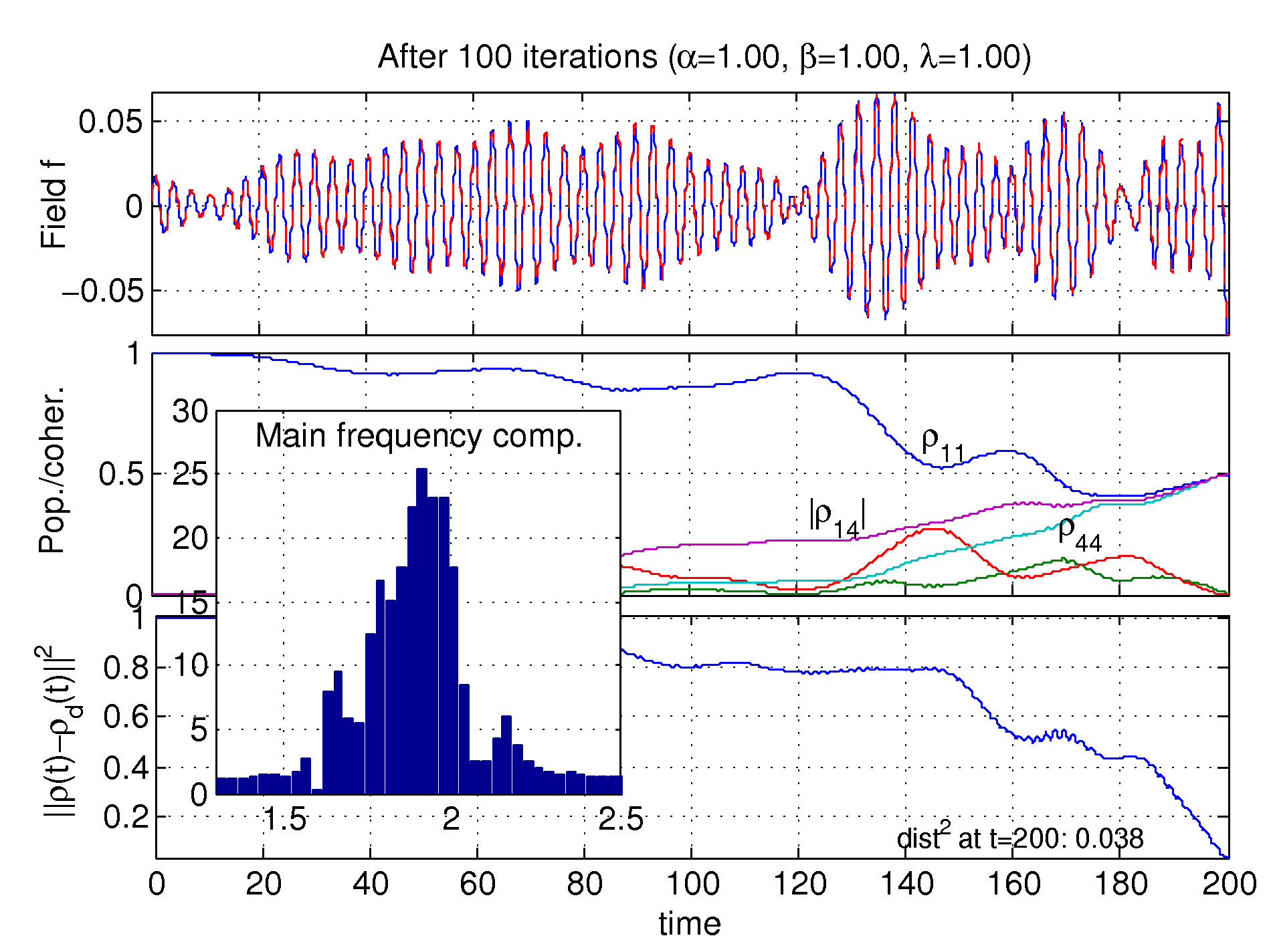
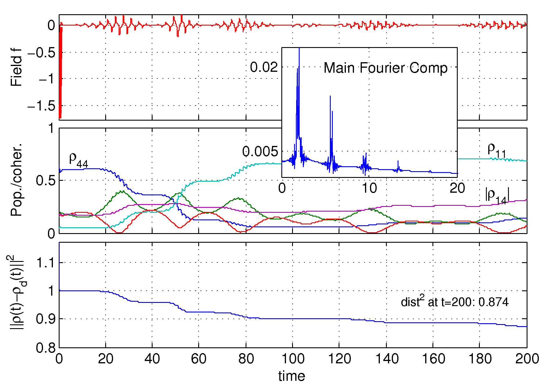
Figure 3: Control pulse, corresponding evolution of the populations $\rho_{kk}$, $k=1,2,3,4$, and crucial coherence $|\rho_{14}|$, and distance from the target state as a function of time for an optimal control pulse obtained from an iterative scheme (top) and a Lyapunov-derived pulse (bottom). Insets shows the main Fourier components of the pulse.

The Lyapunov potential approach proved considerably more problematic. Firstly, many initial states of interest such as the separable state $|00\rangle$ in our example, lie within the set of states for which convergence does not occur as $\langle\Psi_{d}(0)|H_{1}|\Psi(0)\rangle=0$, and hence the Lyapunov derived control field $f\equiv 0$. We can overcome this problem by applying a random initial pulse to kick the system out of its initial equilibrium state. Even with this modification, however, in all our experiments the controls derived from the Lyapunov potential function performed significantly worse than those derived from iterative schemes, both in terms of the rate of convergence to the target state, and the characteristics of the pulses. In fact, in our example, the distance from the target trajectory, although monotonically decreasing as a function of time, exhibits plateaux where the system appears to be trapped in ’false’ semi-stable states for long periods of time. Furthermore, the control fields we obtained, a typical example of which is shown in Fig. 3 (bottom), tended to be generally spiky and spectrally more complex than those derived from iterative schemes.

In our particular example (and a number of other cases we have studied so far) we found that the iterative algorithm allowed us to find control pulses that steer the system to a state very close to the target state in a relatively short time, as Fig. 3 shows. This applied even to some systems that are not generally controllable, provided that the control objective was dynamically realizable, and in cases where it was not attainable, we were often able to steer the system to reachable states that maximized the expectation value of the target observable subject to the dynamical constaints.

The local optimization approach on the other hand, despite recent claims of strong global convergence [12, 13], seemed to fare significantly worse in our simulations. The system often got trapped for long periods in semi-stable critical points, and convergence to the target state was slow at best. Thus, while asymptotic convergence may be an attractive property mathematically, it appears to be less useful in practice, especially where gate-operation and state preparation times are critical, although further work is necessary to assess whether the cases we have studied are anomalous, and whether the performance of the local gradient optimization can be improved, e.g., by choosing different Lyapunov potentials. The latter question is significant as local optimization techniques can in principle be adapted for measurement-based based feedback control in the context of stochastic differential equations [14, 15].

VI Conclusion

We have considered different ways of modelling quantum control systems, formulating open-loop control problems and techniques for solving them. The preliminary results presented here strongly suggest that model-based optimal control design tends to produce control pulses that are more effective, robust and efficient, than simpler schemes based on geometric pulses. However, the quality of the pulses obtained can vary significantly depending on the choice of model, problem formulation and the technique used for control design.

We have seen in particular that control design based on instantaneous minimization of a Lyapunov potential function, despite attractive features such as simplicity and asymptotic convergence properties, tends to produce fields inferior to those obtained from common iterative optimal control schemes in various regards, from rate of convergence to robustness and what might be termed energy and spectral optimality. Preliminary results suggest that iterative optimal control design produces far better results.

Nonetheless, instantaneous optimization techniques remain of interest due to the potential to adapt these techniques in the context of model-based feedback control. More work is necessary to understand how model choice, problem formulation and algorithmic parameters affect the convergence behavior and characteristics of the fields obtained, in particular for instantaneous optimization techniques, and how these characteristics might be improved, e.g., by choosing more sophisticated Lyapunov potentials.

References

- [1] H. M. Wiseman, Quantum theory of continuous feedback, Phys. Rev. A 49, 2133 (1994).
- [2] J. L. Herek et al., Quantum control of energy flow in light. Nature 417, 533 (2002).
- [3] A. Assion et al., Control of chemical reactions by feedback-optimized phase-shaped femtosecond laser pulses, Science 282, 919 (1998).
- [4] G. Turinici, C. Le Bris, H. Rabitz, Efficient algorithms for laboratory discovery of optimal control controls, Phys. Rev. E 70, 016704 (2004).
- [5] B. J. Pearson, J. L. White, T. C. Weinacht, P. H. Bucksbaum, Coherent control using adaptive learning algorithms, Phys. Rev. A 63, 063412 (2001).
- [6] N. Khaneja, R. Brockett, S. J. Glaser, Time-optimal control in spin systems, Phys. Rev. A 63, 032308 (2001).
- [7] Y. Ohtsuki, W. Zhu, H. Rabitz, Monotonically convergent algorithm for quantum control with dissipation, J. Chem. Phys. 110, 9825 (1999).
- [8] S. G. Schirmer, M. D. Girardeau, J. V. Leahy, Efficient algorithm for optimal control of mixed-state systems, Phys. Rev. A 61, 012101 (2000).
- [9] Y. Maday, G. Turinici, New formulations of monotonically convergent quantum control algorithms, J. Chem. Phys. 118, 8191 (2003).
- [10] N. Khaneja, T. Reiss, C. Kehlet, T. Schulte-Herbrueggen, S. J. Glaser, Optimal control of coupled spin dynamics: design of NMR pulse sequences by gradient ascent algorithms, J. Mag. Resonance 172, 296 (2005).
- [11] M. Mirrahimi, P. Rouchon, Trajectory tracking for quantum systems: a Lyapunov approach, in Proceedings of the MTNS04 (2004).
- [12] C. Altafini, Feedback control of spin systems, quant-ph/0601016 (2006).
- [13] C. Altafini, Feedback stabilization of quantum ensembles: a global convergence analysis on manifolds, quant-ph/0506268 (2005).
- [14] C. Altafini, F. Ticozzi, Almost global stochastic feedback stabilization of conditional quantum dynamics, quant-ph/0510222 (2005).
- [15] M. Mirrahimi, R. von Handel, Stabilizing feedback controls for quantum systems, SIAM J. Control Optim. 46, 445-467 (2007).