Hausdorff clustering

Abstract

A clustering algorithm based on the Hausdorff distance is introduced and compared to the single and complete linkage. The three clustering procedures are applied to a toy example and to the time series of financial data. The dendrograms are scrutinized and their features confronted. The Hausdorff linkage relies of firm mathematicl grounds and turns out to be very effective when one has to discriminate among complex structures.

I Introduction

Clustering is the classification of objects into different groups according to their degree of similarity fukunaga . A number of criteria can be used to define this intuitive (and central) concept, leading in general to different partitions. Due to this arbitrariness, clustering is an inherently ill-posed problem, as a given data set can be partitioned in many different ways without any particular reason to prefer one solution to another. It is clear that a clustering technique can be profoundly influenced by the strategy adopted by the observer and his/her own ideas and preconceptions on the problem.

Clustering algorithms can be classified in different ways according to the criteria used to implement them jain0 :

(A) If, for example, one focuses on the solution, a fundamental distinction can be drawn between hierarchical and partitive techniques. Hierarchical methods yield nested partitions, in which any cluster can be further divided in order to observe its underlying structure. Typical examples are the agglomerative and divisive algorithms that produce dendrograms jain . On the other hand, partitional methods provide only one definite partition which cannot be analyzed in further details.

(B) By contrast, if one focuses on data representation, two schemes are possible: central central and pairwise duda ; hofmann clustering. In central clustering, the data are described by their explicit coordinates in the feature space and each cluster is represented by a prototype (for instance, the mean vector and the corresponding spread). In pairwise clustering, the data are indirectly represented by a dissimilarity matrix, which provides the pairwise comparison between different elements. Clearly, the choice of the measure of dissimilarity is not unique and the performance of any pairwise method strongly depends on it.

(C) Finally, if one focuses on the strategy of the algorithm, two approaches can be adopted: parametric and non-parametric clustering. Parametric algorithms are adopted when some a priori knowledge about the clusters is available and this information is used to make some assumptions on the underlying structure of the data. Vice versa, the non-parametric approach to clustering may represent the optimal strategy when there is no prior knowledge about the data. In general, these methods follow some local criterion for the construction of the clusters, such as, for instance, the identification of high density regions in the data space fukunaga .

From the mathematical point of view, given a set of objects $\mathcal{S}\equiv\{s\}$, an allocation function $m:s\in\mathcal{S}\rightarrow\{1,2,\dots,k\}$, must be defined so that $m(s)$ is the class label and k the total number of clusters (which we assume to be finite for simplicity); k may be chosen a priori or computed within the algorithm. The aim of a clustering procedure is to select, among all possible allocation functions, the one performing the best partition of the set ${\cal S}$ into subsets $\mathcal{G}_{\alpha}\equiv\{s\in\mathcal{S}:m(s)=\alpha\}$   $(\alpha=1,\ldots,k)$, relying on some measure of similarity. The space of any clustering solution is the set $\mathcal{M}$ of all possible allocation functions.

In this article we will focus on a class of clustering techniques called linkage algorithms. Linkage algorithms are hierarchical, agglomerative and non-parametric methods that merge, at each step, the two clusters with the smallest dissimilarity, starting from clusters made of a single element, ending up in one cluster collecting all data. We will analyze the so-called single and complete linkage methods and will introduce a linkage method based on Hausdorff’s distance. We will use as a mathematical definition of dissimilarity a suitable metric in the space of the partitions of the given data set BBDFPP . Notice that in general a similarity measure need not be a distance in the mathematical sense; on the other hand, if one aims at clustering in a parameter space, a distance could be the best choice because it does not introduce any degree of arbitrariness. It is worth stressing that alternative philosophies are also possible, in which the clustering algorithm is governed by purely topological notions and unveils efficient collective dynamics in animal behavior parisi . A comparison among these methods belongs to the realm of statistical mechanics and is beyond the scope of this article. See virasoro for an excellent discussion.

We will focus on finite sets and clusters, although we will keep our analysis on the metric features of the relevant spaces as general as possible. We will start in Sec. II by reviewing and clarifying some mathematical concepts concerning distance and linkage methods, focusing on the single and complete linkage algorithms in Sec. III. The Hausdorff distance and the related clustering procedure will be introduced in Sec. IV. Section V is devoted to the comparison of the different methods on some data sets, including both a toy problem and a case study on financial time series. Some conclusions are drawn in Sec. VI.

II Preliminares

II.1 Distances and pseudodistances

We start by recalling the mathematical definition of distance. Given a set ${\cal S}$, a distance (or a metric) $\delta$ is a non-negative application

$$\delta:{\cal S}\times{\cal S}\longrightarrow\mathbb{R}_{+}$$ (1)

on $\mathbb{R}_{+}=[0,\infty)$, endowed with the following properties, valid $\forall x,y\in{\cal S}$:

$$\delta(x,y)=0\quad\Longleftrightarrow\quad x=y,$$ (2)

$$\delta(x,y)=\delta(y,x),$$ (3)

$$\delta(x,y)\leq\delta(x,z)+\delta(y,z),\quad\forall z\in{\cal S}$$ (4)

Incidentally, notice that symmetry (3), as well as non-negativity, are not independent assumptions, but easily follow from (2) and the triangular inequality (4). If the triangular inequality is written as

$$\delta(x,y)\leq\delta(x,z)+\delta(z,y),\quad\forall z\in{\cal S},$$ (5)

as is often the case, symmetry (3) must be independently postulated. We will henceforth denote a metric space by $(\mathcal{S},\delta)$.

An application (1) is a pseudometric barile if property (2) is weakened:

$$x=y\quad\Longrightarrow\quad\delta(x,y)=0~{}.$$ (6)

In such a case, distinct elements of the set ${\cal S}$ can be at a null distance. A set endowed with a (pseudo)metric is called a (pseudo)metric space.

II.2 Linkage algorithms

Linkage algorithms are hierarchical methods, yielding a clustering structure that is usually displayed in the form of a tree or dendrogram jain . We will adopt an agglomerative algorithm, where the clusters are linked through an iterative process, whose successive steps are the following. Given a data set ${\cal S}$, made up of $n$ elements, at the first level (leaves of the dendrogram) the number of classes is equal to the number of elements. We assume (without loss of generality) that ${\cal S}$ is a metric space . At the first iteration the two closest elements are clustered together, reducing the number of classes to $n-1$ (if more than two elements are at the closest distance, we pick a random couple among them). At the second iteration one has to tackle the subtler problem of defining a distance between the remaining elements of ${\cal S}$ and the first cluster formed. When this is done, the distances are recomputed and the two closest objects are joined. At the following iterations one has to tackle the much more subtle problem of defining a distance among classes. Clearly, this can be done in a variety of different ways and entails further elements of arbitrariness. Assume that this procedure can be carried out consistently. After $n$ steps, all the points are grouped together in one cluster, corresponding to the whole data set. The agglomerative procedure is reversed in a straightforward way in the so-called divisive approach: starting from one single cluster, this is iteratively divided into smaller and smaller ones, until single elements are obtained.

The most commonly used algorithms of this type are the “complete” and the “single” linkage, that differ in the definition of “distance” between subsets of points. In the next section we will briefly review these two algorithms.

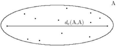
Figure 1: For a set $A$ containing more than one element, $d_{c}(A,A)\neq 0$ and neither (2) nor (6) are valid.

III Complete and Single Linkage

III.1 “Distances”

Linkage algorithms differ from each other for the different similarity criteria used to build the clusters. An optimal criterium would rely on a metric $d$ defined on the subsets of the parent space ${\cal S}$:

$$d:\mathcal{K}({\cal S})\times\mathcal{K}({\cal S})\longrightarrow\mathbb{R}_{+},$$ (7)

where $\mathcal{K}({\cal S})$ is the collection of all the nonempty compact subsets of ${\cal S}$. (We restrict the metric to the above class of subsets in order to avoid some patologies, see later.) Such a metric can be defined in a natural way by using the original metric $\delta$ defined on ${\cal S}$. If $A$ and $B$ are two non empty compact subsets of ${\cal S}$, the complete and single linkage ansatzs make use of the following “distances”

$$d_{c}(A,B)=\sup_{a\in A,b\in B}\delta(a,b),$$ (8)

$$d_{s}(A,B)=\inf_{a\in A,b\in B}\delta(a,b),$$ (9)

respectively. However, it is easy to check that neither one of the above functions is a bona fide distance in the mathematical sense. The function (8) is obviously nonnegative and symmetric, so (3) is valid. Moreover, the triangular inequality (4) is satisfied:

$$d_{c}(A,B) = \sup_{a\in A,b\in B}\delta(a,b)$$ (10)

$$\leq \sup_{a\in A,b\in B,c\in C}(\delta(a,c)+\delta(b,c))$$

$$\leq \sup_{a\in A,b\in B,c\in C}\delta(a,c)+\sup_{a\in A,b\in B,c\in C}\delta(b,c)$$

$$= \sup_{a\in A,c\in C}\delta(a,c)+\sup_{b\in B,c\in C}\delta(b,c)$$

$$= d_{c}(A,C)+d_{c}(B,C)~{}.$$

Yet, property (2) is not valid in general, as for a set $A$ made up of more than one element, the distance of $A$ from itself equals the distance between its farthest objects:

$$d_{c}(A,A)\neq 0~{}.$$ (11)

This is graphically displayed in Fig. 1 and shows that (8) is not even a pseudodistance .

Intuitively, this is not an important issue for “small” sets, but it becomes an increasingly serious problem for “larger” sets. Clearly, the notions of “small” and “large” must be properly defined: for a compact metric space of size $R$, we may say that a subset of size $r$ is small if $r\ll R$ (say by at least one order of magnitude) . This situation will directly concern us in the next sections.

Consider now the second function (9), which is non negative and symmetric, so (3) is valid. Notice that the pseudometric property is satisfied

$$A=B\quad\Longrightarrow\quad d_{s}(A,B)=0,$$ (12)

although the converse is not true [so that property (2) is not valid]: consider for instance two sets $A$ and $B$ such that $A\cap B\neq\varnothing$: in this case $d_{s}(A,B)=0$, as this is, by definition, the distance $\delta$ of a common element from itself. Finally, the triangular inequality (4) is not verified, as can be easily inferred by looking at the counterexample in Fig. 2, for which

$$d_{s}(A,B)>d_{s}(A,C)+d_{s}(B,C).$$ (13)

The function $d_{s}$ is therefore neither a metric nor a pseudometric. As we shall see in Sec. III.3, this problem gives rise to the chaining effect.

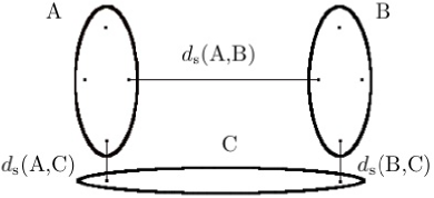
Figure 2: Three sets $A$, $B$, $C$, containing each two elements, for which $d_{s}$ does not satisfy the triangular inequality: $d_{s}(A,B)>d_{s}(A,C)+d_{s}(B,C)$.

III.2 Finite sets

We will look explicitly at the practical case in which (8) and (9) are evaluated on finite sets. It is therefore convenient to specialize the formulas of the preceding section to such a situation. Let $A=\{a_{i}\}_{i=1,\ldots,I}$ and $B=\{b_{j}\}_{j=1,\ldots,J}$ be two finite sets and

$$\delta_{ij}=\delta(a_{i},b_{j})$$ (14)

the distance between any two elements of $A$ and $B$. The $\delta_{ij}$’s can be arranged in a $I\times J$ “distance” matrix. Equations (8) and (9) read then

$$d_{s}(A,B)=\underset{i\in A}{\min}~{}\underset{j\in B}{\min}~{}\delta_{ij},$$ (15)

$$d_{c}(A,B)=\underset{i\in A}{\max}~{}\underset{j\in B}{\max}~{}\delta_{ij},$$ (16)

for the single and complete linkage algorithms, respectively. In practice, this amounts to determine the smaller and the larger value among the rows and the columns of the distance matrix, respectively, a task that can be performed in a polynomial time. These formulas will be applied in the following examples.

III.3 Comments

It is worth commenting on the features of the two clustering ansatzs introduced, emphasizing their limits and positive aspects. The single linkage algorithm tends to yield elongated clusters, which are sometimes difficult to understand and poorly significant jain : this is known as chaining effect. On the contrary, the complete linkage has the advantage of clustering “compact” groups and produces well localized classes. In general, the partitions obtained using it are more significant. Its major disadvantage is that it does not set equal to zero the distance of a “compact” set from itself [see Eq. (11) and Fig. 1], performing de facto a coarse graining. In few words, $d_{c}$ looks at the data points with a “minimal resolution” (that is also, unfortunately, cluster dependent) and is unable to recognize the complexity of a finely structured cluster and to extract “nested” clusters, such as those displayed in Fig. 3 domany . Notice that, by contrast, such “nested” clusters are very efficiently detected by the single linkage algorithm, as shown in Fig. 3.

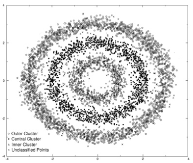
Figure 3: Concentric clusters analyzed in terms of the single linkage algorithm. This procedure is very efficient in discriminating nested structures of this kind. For the same reason, it suffers from the so-called “chaining effect.”

In the next section we shall introduce a procedure that is somewhat “in between” single and complete linkage and makes use of an underlying bona fide distance. This will have some advantages, also from a conceptual viewpoint, as it enables one to rest on firm mathematical background.

IV Hausdorff distance and Hausdorff linkage

In the light of the discussion of the preceding section, it appears convenient to approach the clustering problem from a “neutral” perspective, by looking for a linkage algorithm based on a well-defined mathematical similarity criterium. In order to do this, we will use a distance function introduced by Hausdorff hausdorff .

IV.1 Hausdorff distance

Given a metric space $({\cal S},\delta)$, the distance between a point $a\in{\cal S}$ and a (nonempty and compact) subset $B\in\mathcal{K}({\cal S})$ is naturally given by

$$\tilde{d}(a;B)=\inf_{b\in B}\delta(a,b)$$ (17)

Given a subset $A\in\mathcal{K}({\cal S})$, consider the function

$$\tilde{d}(A;B)=\sup_{a\in A}\tilde{d}(a;B)=\sup_{a\in A}\inf_{b\in B}\delta(a,b),$$ (18)

that measures the largest distance $\tilde{d}(a;B)$, with $a\in A$. Note that here the strategy is opposite to that used with the single linkage “distance” (9), where one considers instead the smallest distance $\tilde{d}(a;B)$, with $a\in A$. The function (18) is not symmetric, $\tilde{d}(A;B)\neq\tilde{d}(B;A)$, and therefore is not a bona fide distance, as it does not satisfy (3). The Hausdorff distance hausdorff between two sets $A,B\in\mathcal{K}({\cal S})$ is defined as the largest between the two numbers:

$$d_{\rm H}(A,B)=\max\{\tilde{d}(A;B),\tilde{d}(B;A)\},$$ (19)

namely,

$$d_{\rm H}(A,B)={\max}\{\sup_{a\in A}\inf_{b\in B}\delta(a,b),\sup_{b\in B}\inf_{a\in A}\delta(a,b)\},$$ (20)

that is clearly symmetric and satisfies all axioms (2)-(4).

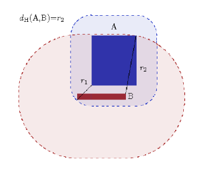
Figure 4: Hausdorff distance between two sets $A$ (a square) and $B$ (a rectangle). The open neighborhoods $N_{r_{1}}(A)$ and $N_{r_{2}}(B)$ are shaded, $r_{1}=\tilde{d}(B;A)$, $r_{2}=\tilde{d}(A;B)$. The Hausdorff distance is $r_{2}$.

It is worth discussing a bit more the mathematical features of $d_{\rm H}$. This will help us grasp its interesting properties, towards physical applications.

Given a set $A\in\mathcal{K}({\cal S})$ and a positive real number $r>0$, define the open r-neighborhood of $A$ as:

$$N_{r}(A)=\{y:\tilde{d}(y;A)<r\}~{}.$$ (21)

The Hausdorff distance between two sets $A,B\in\mathcal{K}({\cal S})$ can be reexpressed as

$$d_{\rm H}(A,B)={\inf}\{r:A\subseteq N_{r}(B)~{}\mbox{and}~{}B\subseteq N_{r}(A)\}~{}.$$ (22)

Indeed

$$d_{\rm H}(A,B)$$

$$={\inf}\{r:A\subseteq N_{r}(B),~{}B\subseteq N_{r}(A)\}$$

$$={\inf}(\{r:A\subseteq N_{r}(B)\}\cap\{r:B\subseteq N_{r}(A)\})$$

$$={\max}\{{\inf}\{r:A\subseteq N_{r}(B)\},~{}{\inf}\{r:B\subseteq N_{r}(A)\}\}$$

and since

$${\inf}\{r:A\subseteq N_{r}(B)\} = \underset{x\in A}{\sup}~{}\inf\{r:x\in N_{r}(B)\}$$ (24)

$$= \underset{x\in A~{}~{}y\in B}{\sup~{}\inf}~{}\delta(x,y)~{},$$

and analogously for ${\inf}\{r:B\subseteq N_{r}(A)\}$, one gets again (20). Stated differently, the Hausdorff distance can also be defined as the smallest radius $r$ such that $N_{r}(A)$ contains $B$ and at the same time $N_{r}(B)$ contains $A$.

In words, the Hausdorff distance between $A$ and $B$ is the smallest positive number $r$, such that every point of $A$ is within distance $r$ of some point of $B$, and every point of $B$ is within distance $r$ of some point of $A$. The geometrical meaning of the Hausdorff distance is best understood by looking at an example, such as that in Fig. 4. We emphasize that the Hausdorff metric on the subsets of ${\cal S}$ is defined in terms of the metric $\delta$ on the points of ${\cal S}$.

The Hausdorff distance enjoys a number of interesting features, that are worth discussing. We have defined $d_{\rm H}$ only on nonempty compact sets for the following reasons. Consider for example the real line. Then, by adopting the convention ${\inf}\{\varnothing\}=\infty$ , one gets $\forall x,d_{\rm H}(\varnothing,x)=\infty$, which is not allowed by any definition of metric. This suggests that we should restrict our attention to nonempty sets. Moreover, $d_{\rm H}(\{0\},[0,\infty))=\infty$, which is again not allowed. We then restrict the use of $d_{\rm H}$ only to bounded sets. Finally, the Hausdorff distance between two not equal sets could vanish [which would make $d_{\rm H}$ a pseudometric, see (6)]: for instance $d_{\rm H}((0,1),[0,1])=0$. Therefore we will restrict the application of $d_{\rm H}$ only to closed sets.

More generally, it is easy to prove the following
Theorem: The Hausdorff function $d_{\rm H}$ is a metric on the set ${\cal K}({\cal S})$. Moreover, if $({\cal S},\delta)$ is a complete metric space, then the space $({\cal K}({\cal S}),d_{\rm H})$ is also complete.

Although of an abstract nature, this is of physical significance, as it enables one to be confident about the metric properties of ${\cal K}({\cal S})$ even for fine-structured clusters. Notice that the property of completeness could not even be conceived for the “distance” $d_{c}$ used for the complete linkage in the last section. In conclusion,

$$d_{\rm H}:{\cal K}({\cal S})\times{\cal K}({\cal S})\longrightarrow\mathbb{R}_{+}$$ (25)

is a complete metric. In the cases of interest, ${\cal S}$ will be a complete metric space, e.g., an Euclidean space.

We close this section with two remarks. First, if the data set is finite and consists of $N$ elements, all distances can be arranged in a $N\times N$ matrix $\delta_{ij}$ and Eq. (20) reads

$$d_{\rm H}(A,B)=\max\{\max_{i\in A}\min_{j\in B}\delta_{ij}~{},\max_{j\in B}\min_{i\in A}\delta_{ij}\},$$ (26)

which is a very handy expression, as it amounts to finding the minimum distance in each row (column) of the distance matrix, then the maximum among the minima. The two numbers are finally compared and the largest one is the Hausdorff distance. This sorting algorithm is efficient and can be easily implemented.

Second, $\forall A,B\in\mathcal{K}({\cal S})$

$$d_{s}(A,B)\leq d_{\rm H}(A,B)\leq d_{c}(A,B).$$ (27)

This is a simple consequence of (20) and the definitions (8) and (9) [or (26), (16) and (15) in the discrete case]. In some sense, $d_{c}$ overestimates the distance between two given sets, essentially because it includes in such a distance the very “size” (11) of the set (see Fig. 1). On the other hand, $d_{s}$ underestimates it. As we shall see, this has important consequences when one clusters complex and/or large sets.

IV.2 Hausdorff linkage

We shall take the Hausdorff distance as our dissimilarity measure. This distance naturally translates in a linkage algorithm: at the first level each element is a cluster, the Hausdorff distance between any pair of points reads

$$d_{\rm H}(\{i\},\{j\})=\delta_{ij}$$ (28)

and coincides with the underlying metric. The two elements of ${\cal S}$ at the shortest distance are then joined together in a single cluster. The Hausdorff distance matrix is recomputed, considering the two joined elements as a single set. This iterative process goes on until all points belong to a single final cluster.

Clearly, when evaluating distances among single elements (points), the three procedures $d_{\rm H}$, $d_{s}$, $d_{c}$ yield the same result. The output of the single linkage algorithm will clearly differ very quickly from the other two, due to the drawbacks of the chaining effect. On the other hand, the differences between Hausdorff and complete linkage will become apparent only later in the clustering process. This is a consequence of the fact that the functions $d_{\rm H}$ and $d_{c}$ yield the same value when evaluated on a single element $\{a\}$ and a composite set $B$. Indeed, from (20):

$$d_{\rm H}(\{a\},B)$$

$$={\max}\{\underset{x\in\{a\}~{}y\in B}{\sup~{}\inf}~{}\delta(x,y),\underset{~{}~{}y\in B~{}x\in\{a\}}{\sup~{}\inf}\delta(x,y)\}$$

$$={\max}\{\underset{y\in B}{\inf}~{}\delta(a,y),~{}\underset{y\in B}{\sup}~{}\delta(a,y)\}$$

$$=\underset{y\in B}{\sup}~{}\delta(a,y)$$

$$=d_{c}(\{a\},B)~{}.$$ (29)

As a consequence of this property, at the lowest levels the Hausdorff linkage will yield a partition that is very similar to that obtained by the complete linkage algorithm. As the clustering procedure goes on, the two methods will differ from each other, because of their different criteria in evaluating distances, leading to different aggregations of more complex classes. It is at this point that the output of the complete linkage becomes less reliable, as a consequence of (11) and (27). As discussed after Eq. (11), we expect this problem to become serious for “large” sets, of size comparable to that of the parent space.

The partitions obtained by the Haudorff linkage algorithm will be intermediate between those obtained by the other two procedures. We shall now compare the three clustering methods, first on an artificial set of points in a two dimensional Euclidean space, then on financial time series.

A final comment is in order. Given a distance matrix, any clustering procedure will yield a tree and an ultrametric, entailing a loss of information on the data set. However, this appears necessary and is inherent in any clustering procedure.

V Applications

V.1 Two-dimensional data set

Let us analyze the effect of the single, complete and Hausdorff linkage algorithms on the data set shown in Fig. 5. This is a discrete set of points in the plane, resembling a pair of “glasses” (each one made up of 31 points) connected by a short horizontal “bar” (5 points) and two “pupils” (each one made up of 2 points), for a total of $n=71$ points.

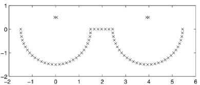
Figure 5: A two-dimensional toy sample: a pair of “glasses” (each one made up of 31 points) connected by a short horizontal “bar” (5 points) and two “pupils” (each one made up of 2 points), for a total of $n=71$ points.

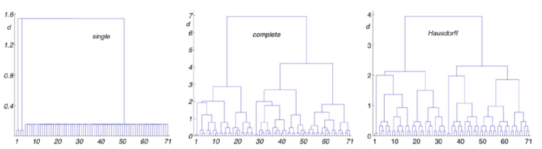
Figure 6: Dendrograms generated by the single, complete and Hausdorff linkage, for the data set of Fig. 5.

This example aims at showing how difficult it can be to discriminate between complete and Hausdorff linkage: while the single linkage will obviously suffer from the chaining effect (and will cluster points at the opposite sides of the figure), the other two procedures will perform in a similar fashion at the beginning, yielding different clusters only when the classes become more complex.

The dendrograms generated by the three algorithms are shown in Fig. 6. The chaining effect of the single linkage is apparent. This can be an advantage if one wants to bring to light the presence of a “continuous” line of points; it is a drawback in a parameter space because data characterized by opposite values of the parameter on the abscissa in Fig. 5 are clustered together. As anticipated, a discrimination between the two other methods is more difficult. However, as discussed after Eq. (11), the differences should become apparent for “large” sets, of size comparable to that of the parent space: for a parent space made up of $n=71$ (approximately linearly distributed) points, we expect this effect to show up for sets made up of more than 7 points, as one can see in Fig. 6.

A proper way to cut the dendrograms could be to search for a stable partition among the whole hierarchy yielded by the algorithms, in correspondence to an approximately constant value of the cluster entropy in a certain range of the dissimilarity measure d kaneko

$$S(d)=-\sum_{k=1}^{N_{d}}P_{d}(k)\ln P_{d}(k)~{},$$ (30)

where $P_{d}(k)$ is the fraction of elements belonging to cluster $k$, and $N_{d}$ the number of clusters at level $d$ in the dendrogram. The complete and Hausdorff entropies corresponding to the dendrograms in Fig. 6 are shown in Fig. 7. We emphasize that, for the case at hand, the data set was intentionally chosen so that one cannot expect an obvious partition into “sensible” clusters. For this very reason, the entropies in Fig. 7 display no “plateau.” The optimal cut is then chosen according to a visual optimization of the clustering solution. Figure 8 shows the selected partitions: while the single linkage yields a clear chaining effect, both complete and Hausdorff methods share the positive aspect of clustering rather “compact” sets. Moreover, all other clusters being roughly similar, the Hausdorff procedure is also able to discriminate the two-points “pupils” in Fig. 5: in this respect it enjoys the positive spin-offs of the single linkage algorithm. On the other hand, the complete linkage algorithm clusters each “pupil” together with a part of its nearest “glass.”

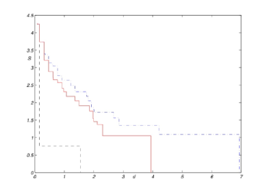
Figure 7: Cluster entropies of the dendrograms of Fig. 6. Dashed black line: single; continuous red line: Hausdorff; blue dot-dashed line: complete.

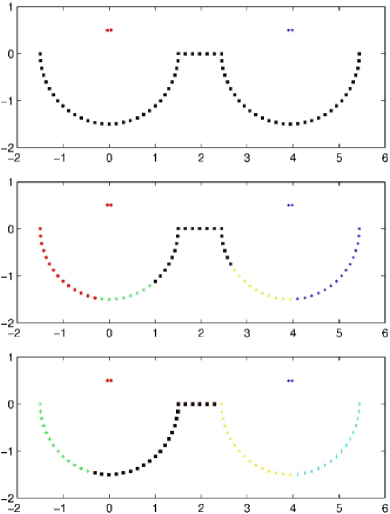
Figure 8: Clustering results for single (up), complete (middle), and Hausdorff (bottom) linkage. Objects belonging to the same cluster share the same symbol: for example the complete algorithm groups the “pupil” on the left (red full circles) with 14 point belonging to its nearest “glass” (red full circles).

V.2 Financial Data

The use of clustering algorithms can improve the reliability of a financial portfolio mantegna_cluster . Here we apply the Hausdorff algorithm to the analysis of financial time series BBDFPP . In particular, we focus on the $N=30$ shares composing the DJIA index, collecting the daily closure prices of its stocks for a period of 5 years (1998-2002). The companies of the DJIA stock market are reported in Appendix A, together with the corresponding industrial areas.

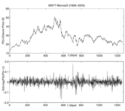
Figure 9: Time evolution of the closure price $P(t)$ and the logarithm of the ratio of consecutive closure prices $X(t)$ [see Eq. (31)] of a stock value (MSFT), for the period 1998-2002.

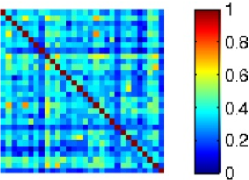
Figure 10: Correlation matrix $\rho(X,Y)$ computed for the year 1998: each element is displayed in a color scale ranging from blu (minimum value) to red (maximum value)

We consider the temporal series of the logarithm of the ratio of two consecutive closure prices

$$X(t)\equiv\ln\frac{P(t)}{P(t-1)},$$ (31)

where $P(t)$ is the closure price of a stock at day $t$. Both $P$ and $X$ are very irregular functions of time, as one can see in Fig. 9, that displays the typical behavior of a stock value (MSFT) for the investigated time period. In order to use the linkage algorithm, we quantify the degree of similarity between two time series X and Y by means of the correlation coefficients computed over the investigated time period:

$$\rho(X,Y)=\frac{\mathrm{cov}(X,Y)}{\sigma_{X}\sigma_{Y}}=\frac{E[(X-\mu_{X})(Y-\mu_{Y})]}{\sigma_{X}\sigma_{Y}}$$ (32)

where $E$ is the expectation value over the time interval of interest (one year in our case), $\mu_{X}=E[X]$ and $\sigma_{X}=\sqrt{E[X^{2}]-\mu_{X}^{2}}$. Figure 10 shows the correlation matrix $\rho(X,Y)$ computed for the year 1998: each element is displayed in a color scale ranging from blu (minimum value) to red (maximum value). It is worth stressing that almost all correlation coefficients are positive, with values not too close to 1, thus confirming that, in many cases, stocks belonging to the same market do not move independently from each other, but rather share a similar temporal behavior.

The metric function we adopted to quantify the time synchronicity between two stocks is the following mantegna ; mant_stan ; Grilli1 :

$$d(X,Y)=\sqrt{2(1-\rho(X,Y))}~{}.$$ (33)

The distance (33) is a proper metric in the parent space, ranging from 0 for perfectly correlated series $[\rho(X,Y)=+1]$ to 2 for anticorrelated stocks $[\rho(X,Y)=-1]$. The representative points lie on a hypersphere and $d(X,Y)$ measures the Euclidean (and not the geodesic) distance between $X$ and $Y$. Figure 11 shows the distance matrix $d(X,Y)$ computed for the year 1998: each element is displayed in a color scale ranging from blu ($d=0$) to red ($d=\sqrt{2}$). The tree structure obtained for this set was already scrutinized and discussed in Ref. BBDFPP . We shall focus here on the features of the dendrograms.

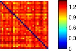
Figure 11: Distance matrix $d(X,Y)$ computed for the year 1998: each element is displayed in a color scale ranging from blu ($d=0$) to red ($d=\sqrt{2}$)

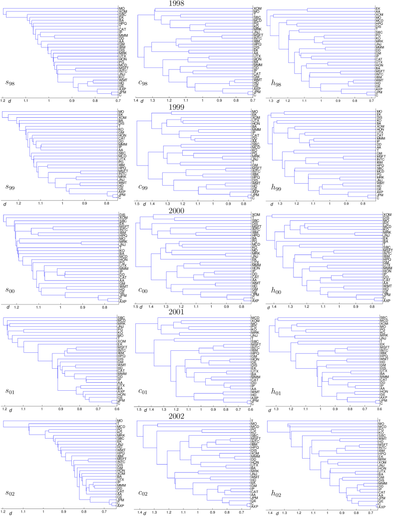
Figure 12: Dendrograms obtained by clustering the stocks from 1998 to 2002 for: single linkage (from $s_{98}$ to $s_{02}$), complete linkage (from $c_{98}$ to $c_{02}$) and Hausdorff linkage (from $h_{98}$ to $h_{02}$). The acronyms are explained in Appendix A. Some “backsteps” can be clearly observed in $h_{02}$. A mathematical explanation of this phenomenon is given in Appendix B.

Figure 12 shows the dendrograms obtained by clustering the stocks yearly from 1998 to 2002, with the single, complete and Hausdorff linkage. Some considerations are in order. As expected, the single linkage algorithm suffers from the chaining effect jain , which yields elongated clusters: different points merge into a large cluster almost one at time during the iterative procedure, with the result of obtaining a poorly defined tree structure, as it can be clearly observed in Fig. 12 (from $s_{98}$ to $s_{02}$). Wherever one would choose to cut the dendrogram, no meaningful partition would emerge out of the hierarchical tree. On the other hand, the dendrograms obtained by means of both the complete and Hausdorff algorithms show clear inner structures, corresponding to the branches of the hierarchical tree. One recognizes the clusters corresponding to homogeneous (from the industrial viewpoint) groups of companies, belonging to the same industrial area: this is the case of the money center banks {C, JPM  AXP}, retail companies {HD, WMT}, companies dealing with basic materials {AA, IP, DD}, and the technological core {IBM, INTC, MSFT}.

The classification of stocks in terms of their economic homogeneity as well as the presence of superclusters and homogeneous subgroups was already discussed in BBDFPP and will not be analyzed here. However, there are characteristic features of the dendrograms that deserve additional attention. An interesting phenomenon, consisting in “backsteps” in the dendrograms, sometimes appears in the Hausdorff clustering, as shown in $h_{02}$ of Fig. 12, the dendrogram obtained by clustering the financial time series in 2002. This pattern is mathematically spelled out in Appendix B, where its significance is elucidated in terms of an elementary example (see Fig. 13). We take this phenomenon as an indicator of the potentialities of a clustering algorithm based on the Hausdorff distance, that could be exploited in a non-hierarchical algorithm, allowing backsteps and hierarchy breaking.

VI Summary

Clustering is a common practice in the analysis of complex data and reflects a human compulsion towards classifying objects or physical phenomena. This can be a difficult task when the phenomena are complicated and the underlying correlations difficult to bring to light. We have introduced and analyzed a clustering procedure based on a bona fide distance introduced by Hausdorff. The method, that relies on an underlying distance among the elements that make up the “parent” set, has been compared with both the single and complete linkage procedures, which only rely on an underlying dissimilarity measure (not a distance). We first looked at a toy problem, in which the Hausdorff method has evident advantages in comparison with the other ones. We then clustered the financial time series of the DJIA stock market, observing the formation of clusters of “homogeneous” companies: the results obtained are significant from an economical point of view.

An important application of the method introduced here is certainly in portfolio optimization elton ; laloux ; onnela2 ; mantegna_cluster ; onnela , where the key issue is to select one (or a few) stocks that are representative of a given cluster, characterized by economic homogeneity, reducing maintenance costs and optimizing risk. Among the possible future developments, one should test the stability of the method against noise effects aste ; tumminello and endeavor to understand the practical consequences of hierarchy breaking due to the backsteps discussed in the previous section.

Appendix A Dow Jones stock market companies

AA:

Alcoa Inc. - Basic Materials

AXP:

American Express Co. - Financial

BA:

Boeing - Capital Goods

C:

Citigroup - Financial

CAT:

Caterpillar - Capital Goods

DD:

DuPont - Basic Materials

DIS:

Walt Disney - Services

EK:

Eastman Kodak - Consumer Cyclical

GE:

General Electrics - Conglomerates

GM:

General Motors - Consumer Cyclical

HD:

Home Depot - Services

HON:

Honeywell International - Capital Goods

HPQ:

Hewlett-Packard - Technology

IBM:

International Business Machine - Technology

INTC:

Intel Corporation - Technology

IP:

International Paper - Basic Materials

JNJ:

Johnson & Johnson - Healthcare

JPM:

JP Morgan Chase - Financial

KO:

Coca Cola Inc. - Consumer Non-Cyclical

MCD:

McDonalds Corp. - Services

MMM:

Minnesota Mining - Conglomerates

MO:

Philip Morris - Consumer Non-Cyclical

MRK:

Merck & Co. - Healthcare

MSFT:

Microsoft - Technology

PG:

Procter & Gamble - Consumer Non-Cyclical

SBC:

SBC Communications - Services

T:

AT&T Gamble - Services

UTX:

United Technology - Conglomerates

WMT:

Wal-Mart Stores - Services

XOM:

Exxon Mobil - Energy

Appendix B

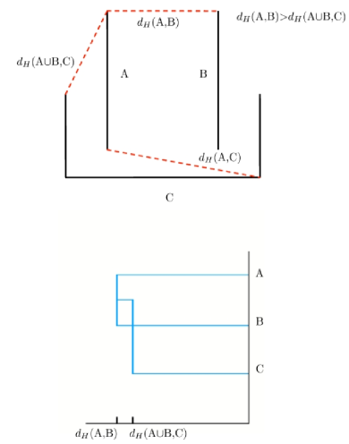
Figure 13: Example of a backstep in the Hausdorff linkage. Given three sets $A$ (a segment), $B$ (another segment) and $C$ (a “U”) , the Hausdorff linkage algorithm links $A$ and $B$ at a distance $d_{\rm H}(A,B)$, then links $A\cup B$ and $C$ at a distance $d_{\rm H}(A\cup B,C)<d_{\rm H}(A,B)$. The set $C$ is nearer to $A\cup B$ than it is to $A$ and $B$ separately. The corresponding dendrogram is drawn below.

We explain here the phenomenon of the backsteps observed in the Hausdorff dendrogram of Fig. 12 (see panel $h_{02}$) and argue that the Hausdorff hierachical clustering does not exploit all the potentialities of the Hausdorff distance.

Let us consider the three compact sets of the Euclidean plane shown in Fig. 13. Set $A$ is a segment, $B$ is another segment and $C$ is a polygonal “U”. They are arranged in such a way that

$$d_{\rm H}(A,B)<d_{\rm H}(A,C),\quad\mathrm{and}\quad d_{\rm H}(A,B)<d_{\rm H}(B,C).$$ (34)

Therefore, the Hausdorff linkage algorithm starts off by linking $A$ and $B$ at a distance $d_{\rm H}(A,B)$ into a cluster $D=A\cup B$. But now it happens that the Hausdorff distance between $C$ and cluster $D$ is smaller than the Hausdorff distance between $A$ and $B$, namely

$$d_{\rm H}(D,C)=d_{\rm H}(A\cup B,C)<d_{\rm H}(A,B).$$ (35)

Therefore, the set $C$ is nearer to $D=A\cup B$ than it is to $A$ and $B$ separately,

$$d_{\rm H}(A\cup B,C)<d_{\rm H}(A,C),\;d_{\rm H}(B,C),$$ (36)

and the corresponding dendrogram exhibits a backstep.

It can therefore happen that two sets, after their aggregation, become Hausdorff-closer to a third set than they were separately. This explains (from a mathematical viewpoint) the phenomenon of the backsteps observed in Fig. 12 (see panel $h_{02})$.

Therefore, backsteps are a direct consequence of the very definition of the Hausdorff distance. The existence of backsteps implies that $d_{\rm H}$ cannot be used as the Hausdorff hierarchy’s aggregation index. Indeed, an aggregation index is a positive function $f$ defined on the hierarchy $Y$ satisfying (i) $f(y)=0$ if and only if $y$ is reduced to a single element of $S$ and (ii) $f(y)<f(y^{\prime})$ if $y\in y^{\prime}$. Equation (36) is at variance with condition (ii). On the other hand, the complete and single hierarchical algorithm generate a hierarchy indexed through $d_{c}$ and $d_{s}$ respectively. Nonetheless, the Hausdorff hierarchy can be indexed through a proper choice of the aggregation index $f$. This will be clarified in a forthcoming article. From a more intuitive (physical) perspective, condition (36) can become valid when the sets are rather intertwined, and can be taken as an indication that, although always mathematically consistent, the clustering procedure itself at this level of the dendrogram becomes doubtful, in particular for inherently complex problems, such as that of clustering stock market companies.

References

- (1) K. Fukunaga: Introduction to Statistical Pattern Recognition. Academic Press, San Diego (1990).
- (2) A.K. Jain, M.N. Murty and P.J. Flynn, ACM Computing Surveys, 31, 264 (1999).
- (3) A. K. Jain, R. C. Dubes: Algorithms for Clustering Data, Prentice Hall, New York (1988).
- (4) A. Gersho, R. M. Gray: Vector Quantization and Signal Processing. Kluwer Academic Publisher, Boston (1992).
- (5) R. O. Duda, P. E. Hart, D. G. Stork: Pattern Classification. John Wiley & Sons, New York (2002).
- (6) T. Hofmann, J. M. Buhmann, IEEE Transaction on Pattern Analysis and Machine Intelligence, 19, 1 (1997).
- (7) N. Basalto, R. Bellotti, F. De Carlo, P. Facchi, E. Pantaleo and S. Pascazio, Physica A 379, 635 (2007).
- (8) M. Ballerini, N. Cabibbo, R. Candelier, A. Cavagna, E. Cisbani, I. Giardina, V. Lecomte, A. Orlandi, G. Parisi, A. Procaccini, M. Viale and V. Zdravkovic, “Interaction Ruling Animal Collective Behaviour Depends on Topological rather than Metric Distance: Evidence from a Field Study”, arXiv:0709.1916 [stat-mech].
- (9) R. Rammal, G. Toulouse, and M. A. Virasoro, Rev. Mod. Phys. 58, 765 (1986).
- (10) J. L. Kelley, General Topology (New York, Van Nostrand, 1955); Eric W. Weisstein et al. “Pseudometric.” From MathWorld–A Wolfram Web Resource. http://mathworld.wolfram.com/Pseudometric.html
- (11) M. Blatt, S. Wiseman, E. Domany, Neural Computation 9, 1805 (1997).
- (12) F. Hausdorff, Grundzüge der Mengenlehre (von Veit, Leipzig, 1914). [Republished as Set Theory, 5th ed. (Chelsea, New York, 2001).]
- (13) K. Kaneko, Phys. Rev. Lett. 63, 219 (1989); Physica D 41, 137 (1990); Physica D 75, 55 (1994).
- (14) V. Tola, F. Lillo, M. Gallegati and R. N. Mantegna, “Cluster analysis for portfolio optimization”, arXiv:physics/0507006 [physics.soc-ph].
- (15) R. N. Mantegna, Eur. Phys. J. B 11, 193 (1999).
- (16) R. N. Mantegna, H. E. Stanley: Introduction to Econophysics. Cambridge University Press (2000).
- (17) M. Bernaschi, L. Grilli and D. Vergni, Physica A 308, 381 (2002); L. Grilli, Physica A 332, 441 (2004).
- (18) E. J. Elton, M. J. Gruber, Modern Portfolio Theory and Investment Analysis (J. Wiley and Sons, 1995).
- (19) L. Laloux, P. Cizeau, J.-P. Bouchaud and M. Potters, Phys. Rev. Lett. 83, 1467, (1999); V. Plerou, P. Gopikrishnan, B. Rosenow, L. A. N. Amaral and H. E. Stanley, Phys. Rev. Lett. 83, 1471, (1999).
- (20) J.-P. Onnela, A. Chakraborti, K. Kaski, J. Kertesz, European Physical Journal B 30, 285 (2002).
- (21) J.-P. Onnela, A. Chakraborti, K. Kaski, J. Kertesz and A. Kanto, Phys. Rev. E 68, 056110 (2003).
- (22) M. Tumminello, T. Aste, T. Di Matteo, R. N. Mantegna, Proc. Nat. Acad. Sci. USA 102, 10421 (2005).
- (23) M. Tumminello, F. Lillo, R. N. Mantegna, Phys. Rev. E 76, 031123 (2007).