Statistics of local density of states in
the Falicov-Kimball model with local disorder

Abstract

Statistics of the local density of states in the two-dimensional Falicov-Kimball model with local disorder is studied by employing the statistical dynamical mean-field theory. Within the theory the local density of states and its distributions are calculated through stochastic self-consistent equations. The most probable value of the local density of states is used to monitor the metal-insulator transition driven by correlation and disorder. Nonvanishing of the most probable value of the local density of states at the Fermi energy indicates the existence of extended states in the two-dimensional disordered interacting system. It is also found that the most probable value of the local density of states exhibits a discontinuity when the system crosses from extended states to the Anderson localization. A phase diagram is also presented.

I Introduction

Electron interaction and disorder strongly influence the properties of materials. In particular, the motion of charge carrier particles can be suppressed by Coulomb interaction and disorder, and the suppression leads to a metal-insulator transition (MIT). In the pure system without disorder the MIT can occur and is purely driven by electron correlations.Mott The transition is commonly referred to the Mott-Hubbard MIT. In the presence of disorder, the MIT can occur even without electron interactions. The state of system changes from extended phase to the Anderson localization due to coherent backscattering from randomly distributed impurities.Anderson The Mott-Hubbard MIT is characterized by opening a gap of the density of states (DOS) at the Fermi energy, while the Anderson localization is a gapless insulator. At the Anderson localization the spectra change from continuous to dense discrete points. It is characterized by vanishing of the most probable value of the local density of states (LDOS).Anderson ; Anderson1 ; Anderson2 The most probable value of the LDOS discriminates between the metal and insulator phases. The importance of the distribution of the LDOS in the proper description of the Anderson localization was stressed by Anderson.Anderson ; Anderson1 ; Anderson2 The very distribution of the LDOS determines the Anderson localization but not average quantities of the LDOS. From the distribution of the LDOS one can detect both the vanishing of the most probable value of LDOS as well as the gap opening of the total DOS, thus the distribution of the LDOS is a valuable tool for determining the MIT driven by both disorder and correlation.

In recent years, a generalized Curie-Weiss mean-field theory, the dynamical mean-field theory (DMFT) was developed.GKKR The DMFT essentially captures local temporal fluctuations. It has been widely applied to study correlated electron systems. The DMFT describes the Mott-Hubbard MIT well.GKKR However, it works with the arithmetic average of the LDOS, and cannot determine the Anderson localization in disordered systems. A statistical variant of the DMFT, which is usually referred to the statistical DMFT, has been introduced to study systems with both disorder and interaction.Dobrosavljevic ; Dobrosavljevic2 It can be viewed as the DMFT formulated in real space with general inhomogeneous solutions.Tran Within the statistical DMFT, the self energy is a local function of frequency, but it also depends on the site index. In the presence of diagonal disorder, the self energy is also diagonal random variables, and gives additional dynamical random contributions to disorder. It generates a set of self-consistent stochastic equations. The statistical DMFT essentially deals with the LDOS, hence it is capable of studying the Anderson-Mott-Hubbard MIT. In parallel with the statistical DMFT, a typical medium theory (TMT) was also introduced to study the Anderson localization.Dobrosavljevic1 The TMT is based on the DMFT too. However, instead of the arithmetic average DOS, it works with the geometric average DOS. The geometric average DOS is incorporated into the self-consistent stochastic DMFT equations, which result into self-consistent equations of the DMFT fashion. The TMT is essentially a mean-field theory of both disorder and correlation, while in the statistical DMFT disorder is treated exactly, and only the correlation effects are treated in a mean-field manner. The TMT was employed to study the Anderson-Mott-Hubbard MIT in correlated electron systems with local disorder.Byczuk ; Byczuk1

In the presence of disorder the LDOS forms a stochastic ensemble. The stochastic ensemble of the LDOS must have characteristics which discriminate between the metallic and insulator phases, and one has to search the characteristics for determining the MIT. Examples for the characteristics are the most probable value of the LDOS in the original Anderson theory of localizationAnderson ; Anderson1 ; Anderson2 or the geometric average of the LDOS in the TMT.Dobrosavljevic1 However, nearby the critical point of the MIT, quantum fluctuations may induce outliers of the statistical description of the stochastic ensemble of the LDOS. For a random sample an estimator is called robust if it is insensitive to outliers.Bickel The most probable value, arithmetic average, median are the examples of robust estimator. The geometric average is not a robust estimator because it does not fulfil the linear property of the robust estimator.Bickel From the point of view of robust statistics the most probable value is a better estimator of a random sample than the geometric average. Moreover, in general, the geometric average DOS is not the most probable value of the LDOS, hence it does not truly represent a typical DOS, although it is closer to the most probable value of the LDOS than the arithmetic average of the LDOS. The geometric average DOS is sensitive to small values of the LDOS at individual sites, even when these values do not represent the most probable value of the LDOS. A decline of the geometric average DOS with increasing the disorder strength does not necessarily imply the approach to the Anderson localization.Song Nevertheless, when the geometric average is embedded into the self-consistent cycle of the DMFT, the whole method, i.e the TMT, can describe the Anderson localization.Dobrosavljevic1 ; Byczuk ; Byczuk1

The interplay between disorder and correlation in the MIT theory is a long standing problem. In the clean or noninteracting limits the MIT was well studied.GKKR ; Lee However, the correlation effects in disordered systems still remain unclear. In particular, despite experiments found evidences of the metallic behavior in the two dimensional electron systems, in theory it is not clear how electron correlations induce metallic phase in low dimensional disordered systems.Kravchenko In the present paper we consider the interplay of disorder and short range interaction in the MIT. Usually, the short range interaction is modelled by the Hubbard interaction.Hubbard Here we take an alternative point of view. Rather than try to study the Hubbard model we take a simpler model, the spinless Falicov-Kimball model (FKM).Falicov The relation of the FKM to the Hubbard model is analogous to the relation between the Ising and Heisenberg models of magnetism. The FKM describes itinerant electrons interacting via a repulsive contact potential with localized electrons (or ions). It can also be viewed as a simplified Hubbard model where electrons with down spin are frozen and do not hop. Certainly, within the TMT the phase diagram of the Anderson-Mott-Hubbard MIT in the FKM and that in the Hubbard model share common features.Byczuk ; Byczuk1 Moreover, the FKM exhibits a rich phase diagram. In homogeneous phase it exhibits the Mott-Hubbard type of MIT, although the model does not describe the Fermi liquid picture. At low temperature different phases with long-range order may exist depending on the doping and interaction strength.Kennedy ; Uelt ; Freericks The FKM can also be incorporated into different models to study various aspects of electron correlations, for instance the charge ordered ferromagnetism in manganites.Tran1 ; Tran2 ; Ramak In the disordered FKM we can study different realizations of the interplay of disorder and electron correlations. With local disorder the FKM exhibits the Anderson-Mott-Hubbard MIT.Byczuk1 It will be studied in the present paper by employing the statistical DMFT. After solving of the self-consistent equations of the statistical DMFT we obtain the distributions of the LDOS. We determine the most probable value of the LDOS and use it to monitor the Anderson localization. We find extended states which occur in the region from weak to intermediate strengths of interaction and disorder. For intermediate values of disorder or interaction there is a reentrance of the Anderson localization. At strong disorder the system is a gapless insulator, while at strong interaction the system is a Mott-Hubbard insulator. We also find at the crossing point from extended states to localization the most probable value of the LDOS exhibits a discontinuity.

The plan of the present paper is as follows. In Sec. II we present the statistical DMFT through its application to the FKM with local disorder. Numerical results are presented in Sec. III. In Sec. IV conclusion and remarks are presented.

II Statistical dynamical mean-field theory

In this section we describe the statistical DMFT through its application to the FKM with local disorder. The Hamiltonian of the system reads

$$H = \sum_{<i,j>}t_{ij}c^{\dagger}_{i}c_{j}+\sum_{i}\varepsilon_{i}c^{\dagger}_{i}c_{i}-\mu\sum_{i}c^{\dagger}_{i}c_{i}$$ (1)

$$+E_{f}\sum_{i}f^{\dagger}_{i}f_{i}+U\sum_{i}c^{\dagger}_{i}c_{i}f^{\dagger}_{i}f_{i},$$

where $c^{\dagger}_{i}$ ($c_{i}$) and $f^{\dagger}_{i}$ ($f_{i}$) is the creation (annihilation) operator of itinerant and localized electrons at site $i$, respectively. $t_{ij}$ is the hopping integral of itinerant electrons between site $i$ and $j$. In the following we take into account only nearest neighbor hopping, i.e., $t_{ij}=-t$ for nearest neighbor sites, and $t_{ij}=0$ otherwise. We will use $t$ as the energy unit. $U$ is the local interaction of itinerant and localized electrons. $\mu$ is the chemical potential for itinerant electrons. It controls the electron density. $E_{f}$ is the energy level of localized electrons. It also serves as the chemical potential of localized electrons and controls the density of localized electrons. In the following we will consider only the symmetric half filling case. It turns out that it is equivalent to $\mu=U/2$ and $E_{f}=-U/2$.Kennedy $\varepsilon_{i}$ are independent random variables. They represent local disorder in the model. We will consider the random variables with uniform distribution

$$P(\varepsilon_{i})=\frac{1}{W}\Theta\bigg{(}\frac{W}{2}-|\varepsilon_{i}|\bigg{)},$$ (2)

where $\Theta(x)$ is the step function, and $W$ represents the disorder strength. When the disorder is absent, model (1) is the pure FKM. In homogeneous phase which occurs at high temperature it exhibits a Mott-Hubbard MIT.Kennedy ; Uelt ; Freericks When the interaction is absent ($U=0$), itinerant and localized electrons are decoupled, and the itinerant electron part of model (1) represents the Anderson model, and it would exhibit the Anderson localization.Anderson Thus when both disorder and interaction are present, model (1) would exhibit the complex Anderson-Mott-Hubbard MIT transition at high temperature.Byczuk1 The FKM may be realized by loading two kinds of fermion atoms with light and heavy masses in optical lattice. The light atoms play the role of itinerant electrons, while the heavy atoms are kept immobile as the localized electrons.

The main idea of the statistical DMFT is to formulate the DMFT of the system with a realization of disorder in real space.Dobrosavljevic When the disorder is realized, the local Green function is not homogeneous anymore. In this case we can adopt the inhomogeneous DMFTTran for treating the interaction part. Within the approach the disorder is treated exactly, while the effects of electron interaction result into the self energy which is self-consistently calculated by the DMFT equations. However, the self energy depends on the site index. The electron Green function can be written in real space

$$\mathbf{G}(\omega)=[\mathbf{G}_{0}^{-1}(\omega)-\mathbf{\Sigma}(\omega)]^{-1},$$ (3)

where $\Sigma_{ij}(\omega)$ is the self energy of the electron Green function $G_{ij}(\omega)=\langle\langle c_{i}|c^{\dagger}_{j}\rangle\rangle_{\omega}$. $\mathbf{G}_{0}(\omega)$ is the noninteracting Green function. For the FKM with a realization of disorder $\mathbf{G}_{0}(\omega)=[\omega\delta_{ij}-t_{ij}-\varepsilon_{i}+\mu\delta_{ij}]^{-1}$. $\varepsilon_{i}$ is random variables realized accordingly to the probability distribution (2). Equation (3) is just the Dyson equation written in the matrix form. Within the statistical DMFT, the self energy is approximated by a local function of frequency. However, this local function can vary from site to site, i.e.,

$$\Sigma_{ij}(\omega)=\delta_{ij}\Sigma_{i}(\omega).$$ (4)

The approximation is strictly local. In infinite dimensions the self energy is purely local. For finite dimensions the approximation neglects nonlocal correlations. The nonlocal correlations can be systematically incorporated by cluster extensions of the DMFT.Maier The site dependence of the self energy is generated via random variables $\varepsilon_{i}$. As a consequence the self energy $\Sigma_{i}(\omega)$ is also stochastic variables. With this feature the effective mean field and the local Green function also are local stochastic variables. The Dyson equation (3) shows that the self energy gives additional local random contributions to disorder of the system. These contributions are due to both interaction and the interplay between interaction and disorder. However, in difference to the random variables $\varepsilon_{i}$ the contributions are dynamical. They take into account temporal local quantum fluctuations generated by interaction and disorder. They also broaden the random energy levels generated by disorder. The self energy $\Sigma_{i}(\omega)$ is determined from an effective single site. Once the effective single site is solved the self energy is calculated by the Dyson equation

$$\Sigma_{i}(\omega)=\mathcal{G}_{i}^{-1}(\omega)-G_{i}^{-1}(\omega),$$ (5)

where ${\mathcal{G}}_{i}(\omega)$ is the bare Green function of the effective single site and represents the effective mean field acting on site $i$. $G_{i}(\omega)$ is the electron Green function of the effective single site. The self-consistent condition requires that the Green function $G_{i}(\omega)$ of the effective single site must concise with the local Green function of the original lattice. i.e.,

$$G_{i}(\omega)=G_{ii}(\omega).$$ (6)

In the Appendix we show the exact derivation of the self consistent equation for inhomogeneous systems in infinite dimensions. Equations (3)-(6) form the self-consistent system of equations for the lattice Green function and the self energy. They are principal equations of the statistical DMFT. Since the local Green function is stochastic variables, the self-consistent equations are naturally stochastic too. In Eq. (6) the right hand side is a functional of stochastic variables $G_{i}(\omega)$, thus the self-consistent condition (6) generates a stochastic chain of $G_{i}(\omega)$ via the iteration process. The LDOS is defined as usually

$$\rho_{i}(\omega)=-\frac{1}{\pi}\;\text{Im}\;G_{ii}(\omega+i\eta),$$

where $\eta=0^{+}$ is an infinitely small positive number.

For the FKM the effective single site problem has the following action

$$S_{i}[c_{i}^{\dagger},c_{i}] = -\int_{0}^{\beta}d\tau d\tau^{\prime}c_{i}^{\dagger}(\tau)\mathcal{G}_{i}^{-1}(\tau-\tau^{\prime})c_{i}(\tau^{\prime})$$ (7)

$$+\int_{0}^{\beta}d\tau U(c_{i}^{\dagger}c_{i}f_{i}^{\dagger}f_{i})(\tau)+\beta E_{f}f_{i}^{\dagger}f_{i},$$

where $\beta=1/T$ is the inverse of temperature. The partition function corresponding to the action is

$$\mathcal{Z}_{i}=\text{Tr}_{f_{i}}\int\mathcal{D}c_{i}^{\dagger}\mathcal{D}c_{i}e^{-S_{i}[c_{i}^{\dagger},c_{i}]}.$$ (8)

This partition function can be calculated exactly, because the trace over the localized electrons is independent of the dynamics of itinerant electrons. We obtainFreericks

$$\mathcal{Z}_{i}=2\exp\Big{[}\sum_{n}\ln\Big{(}\frac{\mathcal{G}_{i}^{-1}(i\omega_{n})}{i\omega_{n}}\Big{)}e^{i\omega_{n}\eta}\Big{]}+\hskip 42.67912pt$$

$$2\exp\Big{[}-\beta E_{f}+\sum_{n}\ln\Big{(}\frac{\mathcal{G}_{i}^{-1}(i\omega_{n})-U}{i\omega_{n}}\Big{)}e^{i\omega_{n}\eta}\Big{]},$$ (9)

where $\omega_{n}=(2n+1)\pi T$ is the Matsubara frequency. The Green function can directly be calculated from the partition function. Without difficulty one obtains

$$G_{i}(i\omega_{n})=\frac{W_{0i}}{\mathcal{G}_{i}^{-1}(i\omega_{n})}+\frac{W_{1i}}{\mathcal{G}_{i}^{-1}(i\omega_{n})-U},$$ (10)

where $W_{1i}=f(\widetilde{E}_{i})$, $W_{0i}=1-W_{1i}$. Here $f(x)=1/(\exp(\beta x)+1)$ is the Fermi-Dirac distribution function, and

$$\widetilde{E}_{i}=E_{f}+T\sum_{n}\ln\Big{(}\frac{1}{1-U\mathcal{G}_{i}(i\omega_{n})}\Big{)}e^{i\omega_{n}\eta}.$$ (11)

Note that the weight factors $W_{0i}$, $W_{1i}$ are not simply a number. They are functionals of the local Green function. One can show that $W_{1i}=\langle f^{\dagger}_{i}f_{i}\rangle$ is the density of localized electrons at site $i$. So far we have obtained the complete solution of the effective single site. This together with the statistical DMFT equations (3)-(6) fully determine the dynamics of itinerant electrons with a fixed disorder realization. Within the statistical DMFT, the disorder is treated exactly, while the correlation effects are taken into account through the mean field contributions of the DMFT. Once the self-consistent equations of the statistical DMFT are solved we obtain the LDOS. With many different realizations of disorder a data ensemble of the LDOS is obtained. The size of the ensemble depends on the lattice size and the number of disorder realizations. From the ensemble of the LDOS we can determine its probability distributions as well as the most probable value of the LDOS. The most probable value of the LDOS is used to monitor the MIT driven by disorder and correlation.

The present approach proposes a statistical local description of the MIT in disordered interacting systems. The statistical aspect is a proper description since it works directly with the ensemble of LDOS and use the most probable value of the LDOS to monitor the MIT.Anderson ; Anderson1 ; Anderson2 The local treatment in the spirit of DMFT neglects nonlocal correlations. This weakness may be serious in low dimensional systems. However, for the two dimensional FKM nonlocal correlations give nonsignificant contributions to the DOS in the homogeneous phase.Hettler The DMFT calculations for the two-dimensional FKM also show reasonable results.Freericks1 Nevertheless, the statistical DMFT can be considered as a simplest approach incorporating both disorder and correlation to the MIT.

III Numerical results

In this section we present the numerical results of the statistical DMFT equations. In general, the matrix inversion in Eq. (3) can be performed only for a finite size lattice. We consider a two dimensional square lattice with the linear size $L$. Thus, we perform numerical calculations for the lattice of size $L$ and finite number $N_{d}$ of disorder realizations. In particular numerical calculations were performed for $L=12$ and $N_{d}=100$. We take temperature $T=1$ which is high enough for homogeneous phase and avoiding any long-range order. Certainly, the homogeneous phase is insensitive to temperature, however at low temperature it is unstable against the long-range ordered phase.Freericks The Mott-Hubbard like MIT in the FKM occurs only for the homogeneous phase. Strictly speaking, the Anderson localization is well defined only at zero temperature. Here we study the interplay between the Anderson localization and the Mott-Hubbard MIT by investigating the single particle Green function at finite temperature. However, in the absence of long range orders the single particle Green function is insensitive to temperature. Hence, we can consider the single particle Green function at finite temperature as it would be at zero temperature. The symmetric half filling case with fixed $\mu=U/2$ and localized electron density $n_{f}=1/2$ is considered. The energy level $E_{f}$ of localized electrons is determined accordingly by condition $n_{f}=\sum_{i}\langle f^{\dagger}_{i}f_{i}\rangle/L^{2}$ for each disorder realization. We solve the statistical DMFT equations in real frequency by iterations. The small positive number $\eta=0.01$ is used. Without disorder the FKM exhibits the Mott-Hubbard MIT with critical value $U_{c}\approx 4$. Thus when system is clean the system state is metallic for $U<U_{c}$, and is insulator for $U>U_{c}$.

III.1 Total DOS and band edge

Figure 1: The total DOS $\rho_{a}(\omega)$ and its derivative $|d\rho_{a}(\omega)/d\omega|$ for various interactions and disorders.

First we determine the band edge of the system. Usually, the band edge is determined from vanishing condition of the total DOS. The total DOS is defined as the arithmetic average of the LDOS

$$\rho_{a}(\omega)=\frac{1}{N_{d}L^{2}}\sum_{\text{disorder}}\sum_{i}\rho_{i}(\omega).$$ (12)

However, strictly speaking, in the numerical calculations the total DOS never vanishes since $\eta=0.01$ was used. In Fig. 1 we plot the total DOS and its derivative $|d\rho_{a}(\omega)/d\omega|$. One can see that at the band edge the total DOS sharply changes and its derivative exhibits a pronounced peak. We use the position of the peak to determine the band edge. The value of the total DOS at the band edge, $\rho_{be}$, also serves as the cutoff of the DOS. Below this value $\rho_{be}$ the DOS approximately vanishes. For strong interaction and weak disorder, the total DOS opens a gap at the Fermi energy. It is similar to the Mott-Hubbard insulator in the clean case. For such cases we also use the peaks of $|d\rho_{a}(\omega)/d\omega|$ to determine the band gap. For strong interaction and strong disorder, the gap opened at the Fermi energy closes. As we will see later, the system is still localized, but gapless. It is a crossover from the Mott-Hubbard to the Anderson insulator by disorder.

III.2 Anderson-Mott-Hubbard MIT

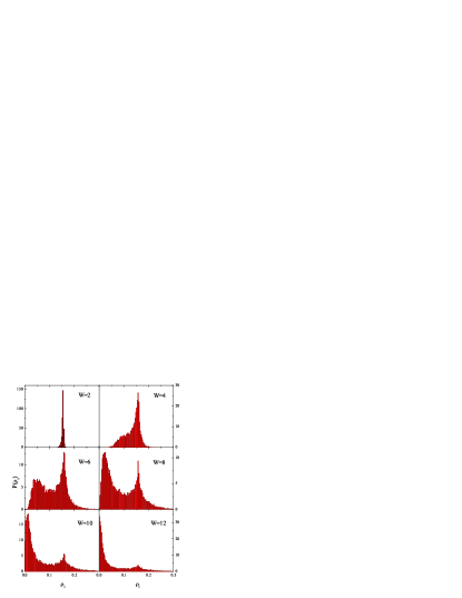
Figure 2: (Color online) Probability distribution $P(\rho_{i})$ of the LDOS $\rho_{i}$ at the Fermi energy for various disorder $W$ in the weak interaction case ($U=2$).

The probability distribution of the LDOS is constructed from statistical data of the LDOS which is obtained after solving the statistical DMFT equations. In Fig. 2 we present the histogram of the probability distribution of the LDOS at the Fermi energy for $U=2$ and various disorders. This value of interaction ($U=2$) corresponds to the metallic phase in the clean limit. For weak disorders the probability distribution has a monomodal structure with a shaped peak at its most probable value. In this regime the most probable value of the LDOS has a finite value, thus the system is in an extended state. This is an unambiguous evidence of the existence of extended states in the two-dimensional disordered interacting system. As the disorder strength increases the peak broadens, and then a second peak is developed. Thus the probability distribution has a bimodal structure. The high value mode is nearly fixed almost independently on the disorder strength. The low value mode moves towards to zero value. Actually, as the disorder strength increases the low value mode becomes the most probable value of the LDOS, and it approximately vanishes at some value of disorder. The vanishing of the most probable value of the LDOS is detected in the sense that its value is below the density cutoff $\rho_{be}$. The vanishing of the most probable value of the LDOS manifests the Anderson localization. Thus the system exhibits a MIT from extended state to the Anderson localization as the disorder strength increases. Perhaps, the bimodal structure of the probability distribution of the LDOS is due to special features of the FKM. The low value mode is due to the Anderson localization when disorder increases. The high value mode reflects the non-Fermi liquid behavior of the FKM in the weak interaction regime. For weak interactions the chemical potential remains pinned at the effective level of $f$ localized electrons.Si In the presence of disorder most of the LDOS still persist with the pinning property, thus most of the LDOS at the chemical potential keep the same value. The bimodal structure may be absent in the systems where the Fermi liquid properties are maintained.

Figure 3: The most probable value $\rho_{\text{mpv}}$, arithmetic average $\rho_{\text{a}}$ and geometric average $\rho_{\text{g}}$ of the LDOS at the Fermi energy via disorder strength $W$ in the weak interaction case ($U=2$).

In principle, we can determine the most probable value as the value at which the probability distribution reaches its global maximum. However, the probability distribution is constructed by histogram, its most probable value is sensitive to the width of histogram bars. To avoid the inaccuracy, we determine the most probable value by the half sample mode algorithm.Bickel This algorithm is a fast routine for locating the most probable value of a finite statistical sample. The half sample mode algorithm is based on finding the smallest interval that contains half number of the sample points. The most probable value must lie in the obtained half sample. Repeat this half sample procedure until obtain the half sample with two or three sample points. Then one can easily locate the most probable value of the sample. In Fig. 3 we plot the most probable value as well as the arithmetic and geometric average of the LDOS at the Fermi energy for comparison. It shows as the disorder strength increases the most probable value shifts from the higher value mode to lower value one. After a critical value of disorder strength ($W_{c}\approx 11.1$) the most probable value approximately vanishes, thus the system changes to the Anderson localized phase. At the crossing point the most probable value exhibits a discontinuity. The most probable value of the LDOS is not an order parameter of MIT, since it does not associate with any symmetry breaking, but the discontinuity of the most probable value of the LDOS may be considered as a sign of the first order phase transition. Figure 3 also shows that both the arithmetic and geometric average of the LDOS never coincide with the most probable value of the LDOS. The arithmetic and geometric averages of the LDOS monotonously decrease as the disorder strength increases. However, the decreases do not necessarily imply the approach to the Anderson localization.Song

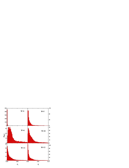
Figure 4: (Color online) Probability distribution $P(\rho_{i})$ of the LDOS $\rho_{i}$ at the Fermi energy for various disorder $W$ in the intermediate interaction case ($U=6$).

In Fig. 4 we present the histogram for the probability distribution of the LDOS at the Fermi energy for various disorders and $U=6$. This value of interaction ($U=6$) corresponds to the insulator phase in the clean limit. In difference to the weak interaction case, at weak disorders the probability distribution of the LDOS at the Fermi energy has almost a delta function like structure. It means that almost all LDOS at the Fermi energy vanish. The total DOS opens a gap at the Fermi energy. It is analogous to the Mott-Hubbard insulator in the clean limit. As the disorder strength increases, the delta peak broadens, and the probability distribution of the LDOS shows a long tail. However, the most probable value of the LDOS still approximately vanishes, while the arithmetic and geometric average are finite. The total DOS now closes the opened gap at the Fermi energy. The system state is still localized, however gapless. It is analogous to the Anderson localized phase in the noninteracting limit. We still refer it to the Anderson localization, although the physics nature may be different. In general, at finite interaction and finite disorder there are no precise definitions of the Mott-Hubbard and Anderson insulating phases.Byczuk These phases rigorously exist only in the clean or noninteracting limits. In disordered interacting systems, both phases are characterized by vanishing of the most probable value of the LDOS at the Fermi energy. However, the total DOS of the Mott-Hubbard insulator opens a gap at the Fermi energy, while the one of the Anderson localization is gapless. The scenario of closing the opened gap by disorder in the strong interaction case can be understood from the atomic limit.Aguiar In the clean atomic limit each site has two energy levels, one single occupancy and one double occupancy, separated by interaction strength $U$. At the half filling, each site is occupied either by one itinerant electron or by one localized electron. The double occupancy levels remain empty, thus the charge gap is equal to $U$. When disorder is added, each of these two energy levels is shifted by randomly fluctuating site energy $-W/2<\varepsilon_{i}<W/2$. For $W<U$ the situation remains unchanged, thus there is still a charge gap for electron excitations. When $W>U$, the double occupancy levels at some sites may be shifted lower than the single occupancy levels. Thus the double occupancy levels of a fraction of sites are either occupied or empty. As a result the charge gap is closed. The phase may be interpreted as a mixture of Anderson and Mott-Hubbard insulators.

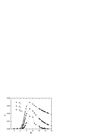
Figure 5: The most probable value $\rho_{\text{mpv}}$, arithmetic average $\rho_{\text{a}}$ and geometric average $\rho_{\text{g}}$ of the LDOS at the Fermi energy via disorder strength $W$ in the strong interaction case ($U=6$).

In contrast to the weak interaction case, where the probability distribution of the LDOS has the bimodal structure, in the intermediate and strong interaction cases the probability distribution of the LDOS keeps its monomodal structure. As the disorder strength increases further, the most probable value of the LDOS first increases from zero value and then decreases back to zero value. In the first stage the system changes from the localized state to extended state, while in the second stage the system changes back from the extended state to localized state. It is a reentry effect of the Anderson localization. In Fig. 5 we plot the most probable value, the arithmetic and geometric average of the LDOS at the Fermi energy as a function of the disorder strength for $U=6$. In difference to the weak interaction case, as the disorder strength increases, the most probable value and the averages of the LDOS increase from zero value, reach their maximum, and then decrease. It also shows that the geometric average of the LDOS approximately vanishes only in the Mott-Hubbard insulator phase. However in this phase the arithmetic average and the most probable value of the LDOS approximately vanish too. In the Anderson localized phase only the most probable value of the LDOS vanishes. In the region of intermediate values of the disorder strength, the most probable value of the LDOS is finite. This evidence unambiguously indicates the existence of extended states for intermediate disorders. It also shows that disorder can drive the system from the insulating state to extended one. However, the insulating state should be the gapless localized state. Disorder cannot drive a Mott-Hubbard insulator directly to extended state. One may speculate the MIT scenario of the intermediate interaction case as a screening of disorder which leads to close the gap at the Fermi energy, and then the standard scenario of the Anderson localization as in the weak interaction case. At the transition point the most probable value also shows a discontinuity like in the weak interaction case. We can use the discontinuity to detect the crossing point from extended to localized states.

Figure 6: Phase diagram for the Mott-Hubbard-Anderson MIT. The dotted line separates the phase region with finite gap in the total DOS.

In Fig. 6 we plot the phase diagram. It clearly distinguishes three phase regions. Extended phase is those states that the most probable value of the LDOS at the Fermi energy is finite. The insulator phase is characterized by the vanishing of the the most probable value of the LDOS at the Fermi energy. This phase is separated into the Anderson localization where the total DOS is gapless and the Mott-Hubbard insulator where the total DOS opens a gap at the Fermi energy. The Anderson localization occurs for strong disorder, while the Mott-Hubbard insulator occurs for strong correlation. The extended phase appears only for weak and intermediate disorder and correlation. For a weak disorder, as the interaction increases, the system changes from the extended phase to the Anderson localization, and finally to the Mott-Hubbard insulator. For an intermediate value of disorder, as the interaction increases, the system changes from the Anderson localization to the extended phase, and then back again to the Anderson localization. This is a reentry effect of the Anderson localization. For a weak interaction as the disorder strength increases the system changes from extended to localized phase. For intermediate and strong interactions there is a crossover from the Mott-Hubbard insulator to the Anderson insulator by closing the gap at the Fermi energy by disorder. For a fixed intermediate interaction there is also the reentry effect of the Anderson localization when the disorder strength is varied. The phase diagram is qualitatively analogous to the one calculated within the TMT.Byczuk1 Although the geometric mean alone does not indicate the Anderson localization, its fully embedding in the self consistent cycle of the DMFT may describe the Anderson localization.Dobrosavljevic1 ; Byczuk ; Byczuk1 However, within the statistical DMFT there is a discontinuity of the most probable value of the LDOS at the phase boundary, whereas within the TMT the geometric average is continuous at the phase boundary. The two limiting cases $W=0$ and $U=0$ are special. In the clean limit $W=0$, there is the Mott-Hubbard MIT, although the metallic phase is not a Fermi liquid. The noninteracting limit $U=0$ is controversial in two dimension. Our result agrees well with the real space renormalization group calculations.Lee1 However, scaling theory did not find any true metallic behavior in the system.Abrahams There is only a crossover from exponentially to logarithmically localized states. Certainly, the present phase diagram is constructed from statistics of the LDOS, and the actual transport properties still remain unclear. Nevertheless, it was demonstrated that the two dimensional disordered Hubbard model can have a delocalizing effect.Denteneer ; Herbut ; Srinivasan ; Heidarian

III.3 Finite size effects

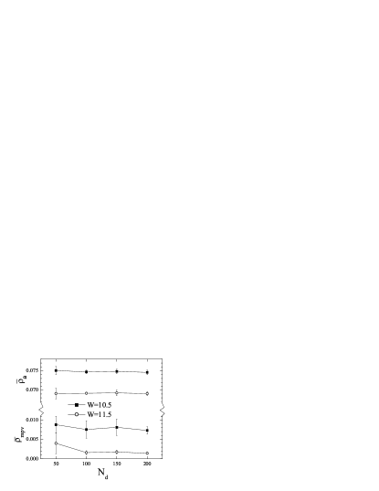
Figure 7: The statistical average of the most probable value (mpv) and the arithmetic average (a) of the LDOS at the Fermi energy via the number of disorder realizations. The error bars are their standard deviations. ($U=2$, $L=12$, $N_{b}=5$).

$L$	$8$	$10$	$12$	$14$	$16$
$N_{d}$	$240$	$150$	$110$	$80$	$60$
$N$	$15680$	$15000$	$15840$	$15680$	$15360$

Table 1: The lattice size $L$, the number of disorder realizations $N_{d}$, and the total number $N$, which are used for study of the finite size effects.

The results of the previous subsections basically permit finite size effects. There are two sources of the finite size effects. One is the finite size $L$ of the lattice, and the second is the finite number $N_{d}$ of disorder realizations. First, we study the finite size effects of $N_{d}$. We fix the lattice size $L=12$, and consider different numbers of disorder realizations. For each $N_{d}$ we generate $N_{b}$ different bins of size $L^{2}N_{d}$ for disorder realizations. For each bin we calculate the most probable value as well as the arithmetic average of the LDOS at the Fermi energy. Then we calculate their statistical average $\overline{\rho}_{\alpha}$ and standard deviation $\sigma_{\alpha}$, i.e.,

$$\overline{\rho}_{\alpha} = \frac{1}{N_{b}}\sum_{n=1}^{N_{b}}\rho_{\alpha}^{(n)},$$

$$\sigma_{\alpha}^{2} = \frac{1}{N_{b}-1}\sum_{n=1}^{N_{b}}\big{(}\rho_{\alpha}^{(n)}-\overline{\rho}_{\alpha}\big{)}^{2},$$

where $\alpha$ denotes the most probable value (mpv) or the arithmetic average (a). $\rho_{\alpha}^{(n)}$ is the most probable value or the arithmetic average of the LDOS, obtained from the nth bin calculations. In Fig. 7 we plot the statistical average and the standard deviation of the most probable value or the arithmetic average of the LDOS at the Fermi energy for various $N_{d}$ and $N_{b}=5$. We choose two values of disorder nearby the transition point. One is in the extended phase, and the other is in Anderson localized phase. Figure 7 shows the arithmetic average of the LDOS (the total DOS) has little fluctuations even for $N_{d}=50$. It almost independent on $N_{d}$ already from $N_{d}=50$. The most probable value of the LDOS fluctuates in the extended phase more strongly than in the localized phase. Certainly, in the localized phase the most probable value of the LDOS approximately vanishes, that the fluctuations of the vanishing value is negligible when $N_{d}$ varies. The most probable value of the LDOS seems to be reasonable from $N_{d}=100$. Thus at $N_{d}=100$ the finite size effects of $N_{d}$ are small and do not significantly change the results.

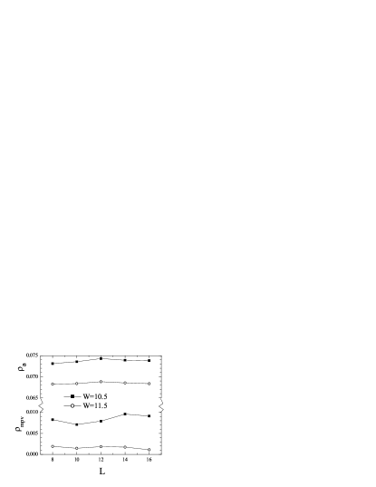
Figure 8: The most probable value $\rho_{mpv}$ and the arithmetic average $\rho_{a}$ of the LDOS at the Fermi energy via the lattice size $L$. The number of disorder realizations for each lattice size is given in Table I. ($U=2$).

Next, we study the finite size effects of the lattice size. The DMFT calculations for clean systems show the finite site effects are small and controllable.Tran In disordered systems, one can notice that the finite size effects of the ensemble of the LDOS depend mostly on the size of the ensemble, i.e., on the number $N=L^{2}N_{d}$. $N$ is the total number of LDOS which are obtained in numerical calculations. Therefore to study the finite size effects of $L$ alone, when the lattice size $L$ is varied, we have to change $N_{d}$ accordingly, that the total number $N$ keeps more or less the same value. In Table I we present several values of $L$, and corresponding values of $N_{d}$ that the total number $N$ is around $15000$. We use the parameter values in Table I for study of the finite size effects of $L$. For all cases the whole bin of disorder realizations is kept more or less the same. We also choose two values of disorder nearby the transition point. One is in the extended phase, and the other is in the localized phase. The most probable value and the arithmetic average of the LDOS at the Fermi energy via the lattice size are plotted in Fig. 8. It shows that the arithmetic average of the LDOS is almost independent on the lattice size, at least from $L=8$. The most probable value of the LDOS also slightly fluctuates as the lattice size varies. These fluctuations mainly are due to the statistical fluctuations of finite size of disorder realizations. As we already showed in Fig. 7, the statistical fluctuations of the most probable value of the LDOS in the extended phase is larger than in the localized phase. This feature is consistent with Fig. 8, where the most probable value of the LDOS fluctuates in the extended phase stronger than in the localized phase. Both results show that the finite size effects in our study are small and do not change significantly the picture of MIT. It is interesting to note that the DMFT can be performed for finite size lattices, and the obtained results are not significantly different from the ones of the thermodynamical limit.Tran

IV Conclusions

In this paper we have studied the Mott-Hubbard-Anderson MIT in the two-dimensional FKM with local disorder by the statistical DMFT. Within the statistical DMFT the correlation effects are resulted into additional dynamical local random variables, which are self-consistently determined from the local single site dynamics. The probability distribution and the most probable value of the LDOS are calculated. The localized phase is detected by vanishing condition of the most probable value of the LDOS at the Fermi energy. The scenario of the MIT in the system depends on the interaction. For weak interactions, which correspond to the metallic phase in the clean limit, the system changes from extended to localized states as the disorder strength increases. For intermediate interactions, which correspond to the insulating phase in the clean limit, as the disorder strength increases the system crosses from the Mott-Hubbard to the Anderson insulator, and then it transits to extended states and goes back again to the Anderson localized phase. Thus there is a reentrance of the Anderson localization. At the crossing point from extended to localized states the most probable value of the LDOS exhibits a discontinuity. For strong interactions only localized states exist. There is only a crossover from the Mott-Hubbard to the Anderson insulator by closing the opened gap at the Fermi energy by disorder. The results also confirm the delocalizing effect in the two dimensional disordered interacting system. However, the phase diagram was determined only by statistics of the LDOS, and the actual transport properties of the system still remain unclear. We leave the problem for further study.

Appendix A Self consistent equation of the inhomogeneous DMFT in infinite dimensions

In this Appendix we present the derivation of the self consistent equation of the inhomogeneous DMFT in infinite dimensions. Formally, we can derive the self consistent equation for inhomogeneous systems in the same way as for homogeneous systems.GKKR Certainly, the derivation for homogeneous systems is based on the cavity method and the Hilbert transform.GKKR Since the cavity method for homogeneous systems is also formulated in real space, we can follow it closely. First a disorder realization is fixed, and then all fermions are traced out except for a single site $l$. In the infinite dimensions we obtain the Green function which represents the effective mean fieldGKKR

$$\mathcal{G}_{l}^{-1}(i\omega_{n}) = i\omega_{n}+\mu-\varepsilon_{l}-\Delta_{l}(i\omega_{n}),$$ (13)

$$\Delta_{l}(i\omega_{n}) = \sum_{ij}t_{li}G^{(l)}_{ij}(i\omega_{n})t_{jl},$$ (14)

where $G_{ij}^{(l)}(i\omega_{n})$ is the Green function of the model with site $l$ removed. $\Delta_{l}(i\omega_{n})$ can be considered as a hybridization function. The cavity Green function can be expressed through the original lattice Green functionGKKR

$$G^{(l)}_{ij}(i\omega_{n})=G_{ij}(i\omega_{n})-\frac{\displaystyle G_{il}(i\omega_{n})G_{lj}(i\omega_{n})}{\displaystyle G_{ll}(i\omega_{n})}.$$ (15)

Inserting Eq. (15) into Eq. (14) one obtains

$$\Delta_{l}(i\omega_{n}) = \big{[}\mathbf{t}\cdot\mathbf{G}(i\omega_{n})\cdot\mathbf{t}\big{]}_{ll}$$ (16)

$$-\frac{\displaystyle\big{[}\mathbf{t}\cdot\mathbf{G}(i\omega_{n})\big{]}_{ll}\big{[}\mathbf{G}(i\omega_{n})\cdot\mathbf{t}\big{]}_{ll}}{\displaystyle G_{ll}(i\omega_{n})},$$

where $\mathbf{t}$ is the hopping matrix. The lattice Green function can be rewritten as

$$\mathbf{G}(i\omega_{n})=\big{[}\mbox{\boldmath{$\xi$}}(i\omega_{n})-\mathbf{t}-\mathbf{\Sigma}(i\omega_{n})\big{]}^{-1},$$ (17)

where $\xi_{ij}(i\omega_{n})=(i\omega_{n}+\mu-\varepsilon_{i})\delta_{ij}$. In infinite dimensions the self energy is purely local,GKKR hence the self energy matrix $\mathbf{\Sigma}(i\omega_{n})$ is diagonal. For homogeneous systems the terms in the right hand side of Eq. (16) are calculated by using the Fourier and Hilbert transforms.GKKR For inhomogeneous systems the Fourier and Hilbert transforms are replaced by the matrix multiplication and inversion in real space. One can notice that

$$\mathbf{t}\cdot\mathbf{G}\cdot\mathbf{t} = \mathbf{t}\cdot\mathbf{G}\cdot\big{[}\mbox{\boldmath{$\xi$}}-\mathbf{\Sigma}-\mathbf{G}^{-1}\big{]}$$ (18)

$$= \mathbf{t}\cdot\mathbf{G}\cdot\big{(}\mbox{\boldmath{$\xi$}}-\mathbf{\Sigma}\big{)}-\mathbf{t},$$

$$\mathbf{t}\cdot\mathbf{G} = \big{[}\mbox{\boldmath{$\xi$}}-\mathbf{\Sigma}-\mathbf{G}^{-1}\big{]}\cdot\mathbf{G}$$ (19)

$$= \big{(}\mbox{\boldmath{$\xi$}}-\mathbf{\Sigma}\big{)}\cdot\mathbf{G}-\mathbf{1}.$$

Using relations (18)-(19), from Eq. (16) we obtain

$$\Delta_{l}(i\omega_{n})=-\big{[}\mbox{\boldmath{$\xi$}}(i\omega_{n})-\mathbf{\Sigma}(i\omega_{n})\big{]}_{ll}$$ (20)

$$+ \Big{[}\big{(}\mbox{\boldmath{$\xi$}}(i\omega_{n})-\mathbf{\Sigma}(i\omega_{n})\big{)}\cdot\mathbf{G}(i\omega_{n})\cdot\big{(}\mbox{\boldmath{$\xi$}}(i\omega_{n})-\mathbf{\Sigma}(i\omega_{n})\big{)}\Big{]}_{ll}$$

$$- \big{[}\big{(}\mbox{\boldmath{$\xi$}}(i\omega_{n})-\mathbf{\Sigma}(i\omega_{n})\big{)}\cdot\mathbf{G}(i\omega_{n})-\mathbf{1}\big{]}_{ll}$$

$$\big{[}\mathbf{G}(i\omega_{n})\cdot\big{(}\mbox{\boldmath{$\xi$}}(i\omega_{n})-\mathbf{\Sigma}(i\omega_{n})\big{)}-\mathbf{1}\big{]}_{ll}/G_{ll}(i\omega_{n}).$$

Here we have used $t_{ll}=0$. Since both matrices $\mbox{\boldmath{$\xi$}}(i\omega_{n})$ and $\mathbf{\Sigma}(i\omega_{n})$ are diagonal, from Eqs. (13) and (20) we obtain

$$\mathcal{G}_{l}^{-1}(i\omega_{n})=\Sigma_{l}(i\omega_{n})+1/G_{ll}(i\omega_{n}).$$ (21)

Equation (21) is just the self consistent equations (5)-(6). It is exact in infinite dimensions for any inhomogeneous system. The above derivation of the self consistent equation can be considered as a generalization of the homogeneous one. In infinite dimensions, the sum in Eq. (14) runs over infinitely many neighbouring sites, that the hybridization function is replaced by its average value. As a consequence, all spatial fluctuations of the environment surrounding a given site are suppressed, thus the Anderson localization is prohibited.Dobrosavljevic2 At infinite dimensions the Anderson localization is absent in any disordered interacting system.

References

- (1) N. F. Mott, Metal-Insulator Transition, 2nd ed. (Taylor and Francis, London, 1990).
- (2) P. W. Anderson, Phys. Rev. 109, 1492 (1958).
- (3) P. W. Anderson, Rev. Mod. Phys. 50, 191 (1978).
- (4) R. Abou-Chacra, P. W. Anderson, and D. J. Thouless, J. Phys. C 6 1734 (1973).
- (5) A. Georges, G. Kotliar, W. Krauth, and M. J. Rozenberg, Rev. Mod. Phys. 68, 13 (1996).
- (6) V. Dobrosavljevic and G. Kotliar, Phys. Rev. Lett. 78, 3943 (1997).
- (7) V. Dobrosavljevic and G. Kotliar, Phil. Trans. R. Soc. Lond. A 356, 57 (1998).
- (8) Minh-Tien Tran, Phys. Rev. B 73, 205110 (2006).
- (9) V. Dobrosavljevic, A. A. Pastor, and B. K. Nikolic, Europhys. Lett. 62, 76 (2003).
- (10) K. Byczuk, W. Hofstetter, and D. Vollhardt, Phys. Rev. Lett. 94, 056404 (2005).
- (11) K. Byczuk, Phys. Rev. B 71, 205105 (2005).
- (12) D. R. Bickel and R. F. Fruhwirth, Comp. Stat. & Data Analysis 50, 3500 (2006).
- (13) Y. Song, W. A. Atkinson, and R. Wortis, Phys. Rev. B 76, 045105 (2007).
- (14) P. A. Lee and T. V. Ramakrishnan, Rev. Mod. Phys. 57, 287 (1985).
- (15) E. Abrahams, S. V. Kravchenko, and M. P. Sarachik, Rev. Mod. Phys. 73, 251 (2001).
- (16) J. Hubbard, Proc. Roy. Soc. (London) A 276, 238 (1963).
- (17) L. M. Falicov and J. C. Kimball, Phys. Rev. Lett. 22 997 (1969).
- (18) T. Kennedy, Rev. Math. Phys. 6, 901 (1994).
- (19) J. K. Freericks, E. H. Lieb, and D. Ueltschi, Phys. Rev. Lett. 88, 106401 (2002).
- (20) J. K. Freericks and V. Zlatic, Rev. Mod. Phys. 75, 1333 (2003).
- (21) Tran Minh-Tien, Phys. Rev. B. 67, 144404 (2003).
- (22) Van-Nham Phan and Minh-Tien Tran, Phys. Rev. B 72, 214418 (2005).
- (23) T. V. Ramakrishnan, H. R. Krishnamurthy, S. R. Hassan, and G. Venketeswara Pai, Phys. Rev. Lett. 92, 157203 (2004).
- (24) T. Maier, M. Jarrell, T. Pruschke, and M. H. Hettler, Rev. Mod. Phys. 77, 1027 (2005).
- (25) M. H. Hettler, M. Mukherjee, M. Jarrell, and H. R. Krishnamurthy, Phys. Rev. B 61, 12739 (2000).
- (26) J. K. Freericks, Phys. Rev. B 48, 14797 (1993).
- (27) Q. Si, G. Kotliar, and A. Georges, Phys. Rev. B 46, 1261 (1992).
- (28) M. C. O. Aguiar, V. Dobrosavljevic, E. Abrahams, and G. Kotliar, Phys. Rev. B 73, 115117 (2006).
- (29) P. A. Lee, Phys. Rev. Lett. 42, 1492 (1979).
- (30) E. Abrahams, P. W. Anderson, D. C. Licciardello, and T. V. Ramakrishnan, Phys. Rev. Lett. 42, 673 (1979).
- (31) P. J. H. Denteneer, R. T. Scalettar, and N. Trivedi, Phys. Rev. Lett. 83, 4610 (1999).
- (32) I. F. Herbut, Phys. Rev. B 63, 113102 (2001).
- (33) B. Srinivasan, G. Benenti, and D. L. Shepelyansky, Phys. Rev. B 67, 205112 (2003).
- (34) D. Heidarian and N. Trivedi, Phys. Rev. Lett. 93, 126401 (2004).