Spin-orbit and tensor mean-field effects on spin-orbit splitting including self-consistent core polarizations

Abstract

A new strategy of fitting the coupling constants of the nuclear energy density functional is proposed, which shifts attention from ground-state bulk to single-particle properties. The latter are analyzed in terms of the bare single-particle energies and mass, shape, and spin core-polarization effects. Fit of the isoscalar spin-orbit and both isoscalar and isovector tensor coupling constants directly to the $f_{5/2}-f_{7/2}$ spin-orbit splittings in ⁴⁰Ca, ⁵⁶Ni, and ⁴⁸Ca is proposed as a practical realization of this new programme. It is shown that this fit requires drastic changes in the isoscalar spin-orbit strength and the tensor coupling constants as compared to the commonly accepted values but it considerably and systematically improves basic single-particle properties including spin-orbit splittings and magic-gap energies. Impact of these changes on nuclear binding energies is also discussed.

I Introduction

In this work we propose and explore two new ideas pertaining to the energy density functional (EDF) methods. First, we suggest a necessity of shifting attention and focus of these methods from ground-state bulk properties (e.g. total nuclear masses) to single-particle (s.p.) properties, and to look for a spectroscopic-quality EDFs that would correctly describe nuclear shell structure. Proper positions of s.p. levels are instrumental for good description of deformation, pairing, particle-core coupling, and rotational effects, and many other phenomena.

On the one hand, careful adjustment of these positions were at the heart of tremendous success of phenomenological mean-field (MF) models, like those of Nilsson, Woods-Saxon, or folded Yukawa [RS80] . On the other hand, similarly successful phenomenological description of nuclear masses, within the so-called microscopic-macroscopic method [Lun03] , relies on the liquid-drop mass surface, which is entirely decoupled from the s.p. structure.

Up two now, methods based on using EDFs, in any of its variants like local Skyrme, non-local Gogny, or relativistic-mean-field (RMF) [Ben03] approach, were mostly using adjustments to bulk nuclear properties. As a result, shell properties were described poorly. After so many years of investigations, a further increase in precision and predictability of all methods based on the EDFs may require extensions beyond forms currently in use. Before this can be fully achieved, we propose to first take care of the s.p. properties, and come back to precise adjustment of bulk properties once these extensions are implemented.

Second, we propose to look at the s.p. properties of nuclei through the magnifying glass of odd-even mass differences. This idea has already been put forward in a seminal paper by Rutz et al. [Rut99a] , where calculations performed within the RMF approach were presented. In this paper we perform analogous analysis for the EDFs based on the Skyrme interactions.

On the one hand, it was recognized long time ago, cf., e.g., Refs. [Ham76aw] ; [Ber80w] , that the theoretical s.p. energies, defined as eigenvalues of the MF Hamiltonian, cannot be directly compared to experiment, because they are strongly renormalized by the particle-core coupling. On the other hand, procedures used to deduce the s.p. energies from experiment [Isa02w] ; [Oro96w] ; [Sch07a] require various theoretical assumptions, by which these quantities cease to result from direct experimental observation. In the past, these theoretical and experimental caveats hampered the use of s.p. energies for proper adjustments of EDFs. However, the odd-even mass differences carry very similar physical information to that given by s.p. energies, and have advantage of being clearly defined, both experimentally and theoretically.

Indeed, experimental difference in mass between an odd nucleus and its lighter even-even neighbor, i.e., the particle separation energy, is an easily available and unambiguous piece of data, which reflects the physical role of the s.p. energy, with all polarizations and couplings taken into account. Similarly, differences of masses between the low-lying excited states in an odd system and lighter even-even neighbor may illustrate effective positions of higher s.p. states. Physical connections between these mass differences and s.p. energies are closest in semi-magic nuclei, which will be studied in the present paper.

In theory, the primary goal of the EDF methods is to describe ground-state energies of fermion systems, i.e., in nuclear-physics applications – masses of nuclei. For odd systems, the EDF methods should give masses of ground states and of several low-lying excited states; the latter being obtained by blocking specific s.p. orbitals. We stress here that in an odd system, separate self-consistent calculations have to be performed for each of the blocked states, so as to allow the system for exploring all possible polarizations exerted by the odd particle on the even-even core. Again, this procedure is clearly defined and entirely within the scope and spirit of the EDF method, which is supposed to provide exact energies of correlated states. Note, that although one here calculates total masses of odd and even systems, the comparison with experiment involves the differences of masses, for which many effects cancel out. Therefore, one can confidently attribute calculated differences of masses to properties of effective s.p. energies, with all polarization effects taken into account, like in the experiment. Again, in semi-magic nuclei such a connection is most reliable.

Following the above line of reasoning, in the present paper we study experimental and theoretical aspects of the spin-orbit (SO) splitting between the s.p. states. In particular, we analyze the role of the SO and tensor MFs in providing the correct values of the SO splittings across the nuclear chart. The paper is organized as follows: In Sect. II we briefly recall basic theoretical building blocks related to the SO and tensor terms of the EDFs and interactions. In Sect. III we discuss in details three major sources of the core polarization: the mass, shape, and spin polarizabilities. In Sect. IV we present a novel method that allows for a firm adjustment of the SO and tensor coupling constants arguing that currently used functionals require major revisions concerning strengths of both these terms. The analysis is based on the $f_{7/2}-f_{5/2}$ SO splittings in three key nuclei, including spin-saturated isoscalar ⁴⁰Ca, spin-unsaturated isoscalar ⁵⁶Ni, and spin-unsaturated isovector ⁴⁸Ca systems, and is subsequently verified by systematic calculations of the SO splittings in magic nuclei. In Sect. V we discuss an impact of these changes on binding energies in magic nuclei. Conclusions of the paper are presented in Sect. VI.

II Spin-orbit and tensor energy densities, mean fields, and interactions

We begin by recalling the form of the EDF, which will be used in the present study. In the notation defined in Ref. [Dob95e] (see Ref. [Per04] for more details and extensions), the EDF reads

$${\mathcal{E}}=\int{\rm d}^{3}{\mathbf{r}}\,{\mathcal{H}}({\mathbf{r}}),$$ (1)

where the local energy density ${\mathcal{H}}({\mathbf{r}})$ is a sum of the kinetic energy, and of the potential-energy isoscalar ($t=0$) and isovector ($t=1$) terms,

$${\mathcal{H}}({\mathbf{r}})=\frac{\hbar^{2}}{2m}\tau_{0}+{\mathcal{H}}_{0}({\mathbf{r}})+{\mathcal{H}}_{1}({\mathbf{r}}),$$ (2)

with

$${\mathcal{H}}_{t}({\mathbf{r}})={\mathcal{H}}^{\text{even}}_{t}({\mathbf{r}})+{\mathcal{H}}^{\text{odd}}_{t}({\mathbf{r}}),$$ (3)

and

$$\mathcal{H}_{t}^{\text{even}} = C^{\rho}_{t}\rho^{2}_{t}+C^{\Delta\rho}_{t}\rho_{t}\Delta\rho_{t}+$$

$$C^{\tau}_{t}\rho_{t}\tau_{t}+C^{J}_{t}{\mathbb{J}}^{2}_{t}+C^{\nabla J}_{t}\rho_{t}{\mathbf{\nabla}}\cdot{\mathbf{J}}_{t},$$

$$\mathcal{H}_{t}^{\text{odd}} = C^{s}_{t}{\mathbf{s}}^{2}_{t}+C^{\Delta s}_{t}{\mathbf{s}}_{t}\cdot\Delta{\mathbf{s}}_{t}+$$

$$C^{T}_{t}{\mathbf{s}}_{t}\cdot{\mathbf{T}}_{t}+C^{j}_{t}{\mathbf{j}^{2}_{t}}+C^{\nabla J}_{t}{\mathbf{s}}_{t}\cdot({\mathbf{\nabla}}\times{\mathbf{j}}_{t}).$$

For the time-even, $\rho_{t}$, $\tau_{t}$, and ${\mathbb{J}}_{t}$, and time-odd, ${\mathbf{s}}_{t}$, ${\mathbf{T}}_{t}$, and ${\mathbf{j}}_{t}$, local densities we follow the convention introduced in Ref. [Eng75] , see also Refs. [Ben03] ; [Per04] and references cited therein.

In particular, the SO density ${\mathbf{J}}$ is the vector part of the spin-current tensor density ${\mathbb{J}}$, i.e.,

$${\mathbb{J}}_{\mu\nu}=\tfrac{1}{3}J^{(0)}\delta_{\mu\nu}+\tfrac{1}{2}\varepsilon_{\mu\nu\eta}{J}_{\eta}+J^{(2)}_{\mu\nu},$$ (6)

with

$${\mathbb{J}}^{2}\equiv\sum_{\mu\nu}{\mathbb{J}}_{\mu\nu}^{2}=\tfrac{1}{3}(J^{(0)})^{2}+\tfrac{1}{2}{\mathbf{J}}^{2}+\sum_{\mu\nu}(J^{(2)}_{\mu\nu})^{2}.$$ (7)

In the context of the present study, the time-even tensor and SO parts of the EDF,

$$\mathcal{H}_{T} = C^{J}_{0}{\mathbb{J}}^{2}_{0}+C^{J}_{1}{\mathbb{J}}^{2}_{1},$$ (8)

$$\mathcal{H}_{SO} = C^{\nabla J}_{0}\rho_{0}{\mathbf{\nabla}}\cdot{\mathbf{J}}_{0}+C^{\nabla J}_{1}\rho_{1}{\mathbf{\nabla}}\cdot{\mathbf{J}}_{1},$$ (9)

are of particular interest.

In the spherical-symmetry limit, the scalar $J^{(0)}$ and symmetric-tensor $J^{(2)}_{\mu\nu}$ parts of the spin-current tensor vanish, and thus

$$\mathcal{H}_{T} = \tfrac{1}{2}C^{J}_{0}J^{2}_{0}(r)+\tfrac{1}{2}C^{J}_{1}J^{2}_{1}(r),$$ (10)

$$\mathcal{H}_{SO} = -C^{\nabla J}_{0}J_{0}(r)\frac{d\rho_{0}}{dr}-C^{\nabla J}_{1}J_{1}(r)\frac{d\rho_{1}}{dr},$$ (11)

where the SO density has only the radial component, ${\mathbf{J}}_{t}=\frac{{\mathbf{r}}}{r}J_{t}(r)$. Variation of the tensor and SO parts of the EDF over the radial SO densities $J(r)$ gives the spherical isoscalar ($t=0$) and isovector ($t=1$) SO MFs,

$$W_{t}^{SO} = \frac{1}{2r}\left(C^{J}_{t}J_{t}(r)-C^{\nabla J}_{t}\frac{d\rho_{t}}{dr}\right){\mathbf{L}}\cdot{\mathbf{S}},$$ (12)

which can be easily translated into the neutron ($q=n$) and proton ($q=p$) SO MFs,

$$W_{q}^{SO} = \frac{1}{2r}\bigg{\{}(C^{J}_{0}-C^{J}_{1})J_{0}(r)+2C^{J}_{1}J_{q}(r)$$

$$-(C^{\nabla J}_{0}-C^{\nabla J}_{1})\frac{d\rho_{0}}{dr}-2C^{\nabla J}_{1}\frac{d\rho_{q}}{dr}\bigg{\}}{\mathbf{L}}\cdot{\mathbf{S}}.$$

Although below we perform calculations without assuming spherical and time-reversal symmetries, here we do not repeat general expressions for the SO mean-fields, which can be found in Refs. [Eng75] ; [Per04] . We also note that, in principle, in this general case, one could use different coupling constant multiplying each of the three terms in Eq. (7). In the present exploratory study, we do not implement this possible extension of the EDF, and we use unique tensor coupling constants $C^{J}_{t}$, as defined in Eq. (II).

Identical potential-energy terms of the EDF, Eqs. (II) and (II), are obtained by averaging the Skyrme effective interaction within the Skyrme-Hartree-Fock (SHF) approximation [Ben03] . By this procedure, the EDF coupling constants $C_{t}$ can be expressed through the Skyrme-force parameters, and one can use parameterizations existing in the literature. It is clear that one can study tensor and SO effects entirely within the EDF formalism, i.e., by considering the corresponding tensor and SO parts of the EDF, Eqs. (8) and (9), and coupling constants $C^{J}_{t}$ and $C^{\nabla J}_{t}$, respectively. However, in order to link this approach to those based on the Skyrme interactions, we recall here expressions based on averaging the zero-range tensor and SO forces [Flo75] ; [Sta77] , see also Refs. [Per04] ; [dob06c] ; [Les07] for recent analyses. Namely, in the spherical-symmetry limit, one has

$${\mathcal{H}}_{T}=\tfrac{5}{8}\left[t_{\text{e}}J_{n}(r)J_{p}(r)+t_{\text{o}}(J_{0}^{2}(r)-J_{n}(r)J_{p}(r))\right],$$ (14)

$${\mathcal{H}}_{SO}=\frac{1}{4}\left[3W_{0}J_{0}(r)\frac{d\rho_{0}}{dr}+W_{1}J_{1}(r)\frac{d\rho_{1}}{dr}\right],$$ (15)

where in Eq. (15) two different coupling constants, $W_{0}$ and $W_{1}$, were introduced following Ref. [Rei95] .

The corresponding SO MFs read

$$W_{q}^{SO} = \frac{1}{2r}\bigg{\{}\tfrac{5}{8}\left((t_{\text{e}}+t_{\text{o}})J_{0}(r)-(t_{\text{e}}-t_{\text{o}})J_{q}(r)\right)$$

$$+\frac{1}{4}\left((3W_{0}-W_{1})\frac{d\rho_{0}}{dr}-2W_{1}\frac{d\rho_{q}}{dr}\right)\bigg{\}}{\mathbf{L}}\cdot{\mathbf{S}},$$

[note that in Ref. [dob06c] , the factor of $\tfrac{1}{2}$ was missing at the $W_{0}$ term of Eq. (4)]. By comparing Eqs. (II) and (II), one obtains the following relations between the coupling constants:

$$C_{0}^{J} = \tfrac{5}{16}(3t_{\text{o}}+t_{\text{e}}),$$ (17)

$$C_{1}^{J} = \tfrac{5}{16}(t_{\text{o}}-t_{\text{e}}),$$ (18)

$$C^{\nabla J}_{0} = -\tfrac{3}{4}W_{0},$$ (19)

$$C^{\nabla J}_{1} = -\tfrac{1}{4}W_{1}.$$ (20)

For further discussion of the Skyrme forces and their relation to tensor components we refer the reader to an extensive and complete recent discussion presented in Ref. [Les07] .

In this exploratory work, we base our considerations on the EDF method and deliberately break the connection between the functional (II), and the Skyrme central, tensor, and SO forces. Nevertheless, in the time-even sector, our starting point is the conventional Skyrme-force-inspired functional with coupling constants fixed at the values characteristic for either SkP [Dob84] , SLy4 [Cha97fw] , or SkO [Rei99fw] Skyrme parameterizations. However, poorly known coupling constants in the time-odd sector (those which are not related to the time-even ones through the local-gauge invariance [Dob95e] ) are fixed independently of their Skyrme-force values. For this purpose, the spin coupling constants $C^{s}_{t}$ are readjusted to reproduce empirical values of the Landau parameters, according to the prescription given in Refs. [Ben02afw] ; [Zdu05xw] , and $C^{\Delta s}_{t}$ are set equal to zero. These variants of the standard functionals are below denoted by SkP_L, SLy4_L, and SkO_L.

Strictly pragmatic reasons, like technical complexity and lack of firm experimental benchmarks, made the majority of older Skyrme parameterizations simply disregard the tensor terms, by setting $C^{J}_{t}\equiv 0$. Recent experimental discoveries of new magic shell-openings in neutron-reach light nuclei, e.g., around $N=32$ [For04] ; [Din05] , and their subsequent interpretation in terms of tensor interaction within the shell-model [Ots01] ; [Ots05] ; [Hon05] , caused a revival of interest in tensor terms within the MF approach [Ots06] ; [dob06c] ; [Bro06] ; [Dob07b] ; [Bri07w] ; [Les07] , which is naturally tailored to study s.p. levels. Indeed, as shown in Ref. [dob06c] , the tensor terms mark clear and unique fingerprints in isotonic and isotopic evolution of s.p. levels and, in particular, in the SO splittings.

In this paper, we perform systematic study of the SO splittings. The goal is to resolve contributions to the SO MF (12) due to the tensor and SO parts of the EDF, and to readjust the corresponding coupling constants $C^{J}_{t}$ and $C^{\nabla J}_{t}$. It is shown that this goal can be essentially achieved by studying the $f_{7/2}-f_{5/2}$ SO splittings in three key nuclei: ⁴⁰Ca, ⁴⁸Ca, and ⁵⁶Ni. Before we present in Sec. IV details of the fitting procedure and values of the obtained coupling constants, first we discuss effects of the core polarization and its influence on the calculated and SO splittings.

III Core-polarization effects

In spite of the fact that the s.p. levels belong to basic building blocks of the MF methods, there is still a vivid debate concerning their physical reality. The question whether they constitute only a set of auxiliary quantities, or represent real physical entities that can be inferred from experimental data, was never of any concern for methods based on phenomenological one-body potentials. Indeed, these potentials were bluntly fitted directly to reproduce the s.p. levels deduced, in one way or another, from empirical information around doubly-magic nuclei, see, e.g., Refs. [Dud81] ; [Sch07a] . In turn, these potentials also appear to properly (satisfactorily) reproduce the one-quasiparticle band-heads in open-shell nuclei, see, e.g., Ref. [Naz90] . This success seems to legitimate the physical reliability of the theoretical s.p. levels within the microscopic-macroscopic approaches.

The debate concerns mostly the self-consistent MF approaches based on the EDF methods or two-body effective interactions. The arguments typically brought forward in this context underline the fact that the self-consistent MFs are most often tailored to reproduce bulk nuclear properties like masses, densities, radii, and certain properties of nuclear matter. Consequently, the underlying interactions are non-local with effective masses $m^{\star}/m\sim 0.8$ [Jeu76w] , what in turn artificially lowers the density of s.p. levels around the Fermi energy. It was pointed out by several authors [Ham76aw] ; [Ber80w] ; [Lit06w] that restitution of physical density of the s.p. levels around the Fermi energy can be achieved only after inclusion of particle-vibration coupling, i.e., by going beyond MF.

Within the effective theories, however, these arguments do not seem to be fully convincing. First of all, an effective theory with properly chosen data set used to fit its parameters should automatically select physical value of the effective mass and readjust other parameters (coupling constants) to this value. Examples of such implicit scaling are well known for the SHF theory including: (i) explicit effective mass scaling of the coupling constants $C^{s}$ and $C^{T}$ through the fit to the spectroscopic Landau parameters [Ben02afw] ; (ii) direct dependence of the isovector coupling constants $C_{1}^{\tau}$ and $C_{1}^{\rho}$ on the isoscalar effective mass through the fit to the (observable) symmetry energy strength [Sat06w2] ; (iii) numerical indications for the $m^{\star}$ scaling of the SO interaction inferred from the $f_{7/2}$-$d_{3/2}$ splittings in $A\sim 44$ nuclei [Zdu05xw] . The differences between various parameterizations of the Skyrme-force (or functional) parameters rather clearly suggest that such an implicit $m^{\star}$ dependence of functional coupling constants is a fact, which is, however, neither well recognized nor understood so far.

Secondly, the use of effective interaction with parameters fitted at the MF level is not well justified in beyond-MF approximation. Rather unavoidable double counting results in such a case, and quantitative estimates of level shifts resulting from such calculations need not be very reliable. It is, therefore, quite difficult to accept the viewpoint that unsatisfactory spectroscopic properties of, in particular, modern Skyrme forces can be cured solely by going beyond MF. On the contrary, the magnitude of discrepancies between the SHF and experimental s.p. levels (see below) rather clearly suggest that: (i) the data sets used to fit the force (or functional) parameters are incomplete and (ii) the interaction/functional should be extended. This is exactly the task undertaken in the present exploratory work. We extend the conventional EDFs based on Skyrme interactions by including tensor terms, and fit the corresponding coupling constants to the SO splittings rather than to masses. The preliminary goal is to improve spectroscope properties of functionals, even at the expense of the quality in reproducing the binding energies.

Empirical energy of a given s.p. neutron orbital can be deduced from the difference between the ground-state energy of the doubly-magic core with $N$ neutrons, $E_{0}(N)$, and energies, $E_{p}(N+1)$ or $E_{h}(N-1)$, of its odd neighboring isotopes having a single-particle (p) or single-hole (h) occupying that orbital, i.e.,

$$\epsilon_{p}(N) = E_{p}(N+1)-E_{0}(N),$$ (21)

$$\epsilon_{h}(N) = E_{0}(N)-E_{h}(N-1),$$ (22)

see, for example, Refs. [Isa02w] ; [Oro96w] ; [Sch07a] and referenced cited therein. Note that the total energies above are negative numbers and decrease with increasing numbers of particles, $E_{h}(N-1)>E_{0}(N)>E_{p}(N+1)$. Similarly, we can define a measure of the neutron shell gap as the difference between the lowest single-particle and highest single-hole energy,

$$\Delta\epsilon_{\text{gap}}(N) = \epsilon_{p}(N)-\epsilon_{h}(N)$$

$$= E_{p}(N+1)+E_{h}(N-1)-2E_{0}(N).$$

Single-particle energies of proton orbitals and proton shell gaps are defined in an analogous way.

Consistently with the empirical definitions, in the present paper, the same procedure is used on the theoretical level [Rut99a] . It means that we determine the total energies of doubly-magic cores and their odd neighbors by using the EDF method, and then we calculate the s.p. energies as the corresponding differences (21) or (22). In this way, we avoid all the ambiguities related to questions of what the s.p. energies really are and how they can be extracted from data. Our methodology simply amounts to a specific way of comparing measured and calculated masses of nuclei. In odd nuclei, one has to ensure that particular s.p. orbitals are occupied by odd particles, but still the calculated total energies correspond to masses of their ground and low-lying excited states. Since here we consider only doubly-magic nuclei and their odd neighbors, the pairing correlations are neglected.

In our calculations, both time-even and time-odd polarizations exerted by an odd particle/hole on the doubly-magic core are evaluated self-consistently. In order to discuss these polarizations, let us recall that the extreme s.p. model, in which ground-state energies are sums of fixed s.p. energies of occupied orbitals, is the model with no polarization of any kind included. In this model, the differences of ground-state energies, Eqs. (21) and (22), are, of course, exactly equal to the model s.p. energies. Having this background model in mind, we can distinguish three kinds of polarization effects:

III.1 Mass polarization effect (time-even)

This effect can be understood as the self-consistent rearrangement of all nucleons, which is induced by an added or subtracted odd particle, while the shape is constrained to the spherical point and the time-odd mean fields are neglected. One has to keep in mind, that none of the s.p. orbitals of a spherical multiplet is spherically symmetric, and therefore, when a particle in such a state is added to a closed core, the resulting state of an odd nucleus cannot be spherically symmetric, and thus cannot be self-consistent. A self-consistent solution can only be realized within the so-called filling approximation, whereupon one assumes the occupation probabilities of all orbitals belonging to the spherical multiplet of angular momentum $j$ and degeneracy $2j+1$, to be equal to $v_{j}^{2}=1/(2j+1)$.

The mass polarization effect is exactly zero when evaluated within the first-order approximation. Indeed, as expressed by the Koopmans theorem [Koo33] , the linear term in variation of the total energy with respect to adding or subtracting a particle is exactly equal to the bare single-particle energy of the core. However, the obtained results do not agree with Koopmans theorem. This is illustrated in Fig. 1, where we compare bare and polarized s.p. energies of the $\nu f_{7/2}$ and $\nu d_{3/2}$ orbitals in ⁴⁰Ca. One can see that for both orbitals there is a quite large and positive mass polarization effect.

The reason for this disagreement lies in the fact that, because of the center-of-mass correction, the standard EDF calculations are not really variational with respect to adding or subtracting a particle. Indeed, in these calculations, the total energy of an $A$-particle system is corrected by the center-of-mass correction [Bei75] ; [Ben00d] ,

$$E_{\text{c.m.}}\simeq E^{\text{dir}}_{\text{c.m.}}=-\frac{1}{A}E_{\text{kin}},$$ (24)

where $E_{\text{kin}}$ is the average kinetic energy of the system. The factor of $\tfrac{1}{A}$ is not varied when constructing the standard mean-field Hamiltonian, and therefore, the Koopmans theorem is violated. Had this variation been included, it would have shifted the mean-field potential and thus all bare s.p. energies in given nucleus by a constant,

$$\epsilon^{\prime}_{i}=\epsilon_{i}+\frac{1}{A^{2}}E_{\text{kin}}.$$ (25)

In ⁴⁰Ca, this shift equals to 0.40 MeV and almost exactly corresponds to the entire mass polarization effect shown in Fig. 1. The remaining mass polarization effect can be attributed to higher-order polarization effects (beyond linear) and to the non-selfconsistency of the filling approximation.

A few remarks about the shift in Eq. (25) are here in order. First, the effect is independent on whether the two-body or one-body center-of-mass correction [Ben00d] is used, and on whether this is done before or after variation. Only the detailed value of the shift may depend on a particular implementation of the center-of-mass correction. Second, the shift induces an awkward result of the mean-field potential going asymptotically to a positive constant and not to zero. Although this may seem to be a trivial artifact, which does not influence the s.p. wave functions and observables, it shows that the standard center-of-mass correction should be regarded as an ill-defined theoretical construct. This fact shows up as an acute problem in fission calculations [Ska06] . Third, whenever the bare s.p. energies are compared to empirical data, this shift must by taken into account. Alternatively, as advocated in the present study, one should compare directly the calculated and measured mass differences. Finally, one should note that the shift is irrelevant when differences of the s.p. energies are considered, such as the SO splittings discussed in Sec. IV.

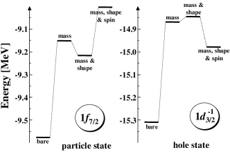
Figure 1: Bare, mass polarized, mass and shape polarized (time-even) and mass, shape and spin polarized s.p. energies of the $\nu f_{7/2}$ particle and the $\nu d_{3/2}^{-1}$ hole in ⁴⁰Ca. The polarized s.p. levels were deduced from binding energies in one particle/hole nuclei according to the formulas (21) and (22). Note that attractive (repulsive) polarization corrections to the binding energies shift the particle state down (up) and the hole state up (down), respectively.

III.2 Shape polarization effect (time-even)

This effect is well known both in the MF and particle-vibration-coupling approaches. Within a deformed MF theory (with the time-odd mean fields neglected), it corresponds to a simple fact that the s.p. energies (eigen-energies in a deformed potential) depend on the deformation in specific way, which is visualized by the standard Nilsson diagram [RS80] . Indeed, in an axially deformed potential, a spherical multiplet of angular momentum $j$ splits into $j+1/2$ orbitals according to moduli of the angular-momentum projections $K=|m_{j}|$. Unless $j=1/2$, for prolate and oblate deformations, orbitals with $K=1/2$ decrease and increase in energy, respectively, while those with maximum $K=j$ behave in an opposite way. Therefore, both for prolate and oblate deformations, and for $j>1/2$, the lowest orbitals have the energies that are lower than those at the spherical point. Hence, a $j>1/2$ particle added to a doubly-magic core always polarizes the core in such a way that the total energy decreases. On the other hand, the energy of a $j=1/2,K=1/2$ orbital does not depend on deformation (in the first order), and thus such an orbital does not exert any shape polarization (in this order).

Exactly the same result is obtained in a particle-vibration-coupling model, in which a $j>1/2$ particle can be coupled with either 0⁺ or 2⁺ state of the core, $[j\otimes 0^{+}]_{j}$ or $[j\otimes 2^{+}]_{j}$, and the repulsion of these two configurations decreases the energy of the ground state with respect to the unperturbed spherical configuration $[j\otimes 0^{+}]_{j}$. As before, for $j=1/2$, the configuration $[j\otimes 2^{+}]_{j}$ does not exist, and the ground state is not lowered.

The above reasoning can be repeated for hole states, with the result that the $j>1/2$ holes added to the doubly-magic core always polarize the core in such a way that the total energy also decreases. As a consequence, the shape polarization effect decreases the s.p. energies of particle states (21) and increases those of hole states (22), and thus decreases the shell gap (III). This effect is clearly illustrated in Fig. 1.

III.3 Spin polarization effect (time-odd)

When an odd particle or hole is added to the core, and the time-odd fields are taken into account, it exerts polarization effects both in the time-even (mass and shape) and time-odd (spin) channels. It means that a non-zero average spin value of the odd particle induces a time-odd component of the mean field, which influences average spin values of all particles, leading to a self-consistent amplification of the spin polarization.

It should be noted at this point that the spin polarization effect dramatically depends on the assumed symmetries and choices made for the occupied orbital, see discussion in the Appendix of Ref. [Olb06] . Indeed, without the time-odd fields, in order to occupy the odd particle or hole, one can use any linear combination of states forming the Kramers-degenerate pair. The total energy is independent of this choice, because the time-even density matrix does not depend on it. This allows for making specific additional assumptions about the conserved symmetries, e.g., in the standard case, one assumes that the odd state is an eigenstate of the signature (or simplex) symmetry with respect to the axis perpendicular to the symmetry axis. However, in order to fully allow for the spin polarization effects through time-odd fields, one has to release all such restrictive symmetries and allow for alignment of the spin of the particle along the symmetry axis. This requires calculations with broken signature symmetry and only the parity symmetry being conserved. Therefore, calculations of this kind are more difficult than those performed within the standard cranking model.

III.4 Total polarization effect

Table 1: Neutron s.p. energies in ¹⁶O, ⁴⁰Ca, and ⁴⁸Ca (in MeV). The columns show: (a) bare unpolarized s.p. energies in doubly-magic cores, (b) self-consistent s.p. energies obtained from binding energies in one-particle/hole nuclei, Eqs. (21) and (22), with time-even mass and shape polarizations included, (c) as in (b), but with time-odd spin polarizations included in addition, and (d) experimental data taken from Ref. [Oro96w] . Time-even, (b)$-$(a), time-odd, (c)$-$(b), and total, (c)$-$(a) polarizations are also shown, along with the differences between the self-consistent and experimental spectra, (c)$-$(d). Positive s.p. energies are shown only to indicate that particular orbitals are unbound in calculations; their values are only very approximately related to positions of resonances. All results have been calculated using the Sly4_L functional.

		bare	T-even	T-even	T-even	T-odd	total	exp.	theory
				pol.	& T-odd	pol.	pol.	[Oro96w]	$-$exp
		(a)	(b)	(b)$-$(a)	(c)	(c)$-$(b)	(c)$-$(a)	(d)	(c)$-$(d)
16O	$1\nu p_{3/2}$	$-$20.57	$-$19.61	0.96	$-$20.29	$-$0.68	0.28	$-$21.84	1.55
	$1\nu p_{1/2}$	$-$14.54	$-$13.55	0.99	$-$13.86	$-$0.31	0.68	$-$15.66	1.80
	$1\nu d_{5/2}$	$-$6.75	$-$5.83	0.92	$-$5.43	0.40	1.32	$-$4.22	$-$1.21
	$2\nu s_{1/2}$	$-$3.78	$-$2.79	0.99	$-$2.30	0.49	1.48	$-$3.35	1.05
	$1\nu d_{3/2}$	0.39	1.19	0.80	1.37	0.18	0.98	1.50	$-$0.13
40Ca	$1\nu d_{5/2}$	$-$22.01	$-$21.55	0.46	$-$21.87	$-$0.32	0.14	$-$22.39	0.52
	$2\nu s_{1/2}$	$-$17.25	$-$16.93	0.32	$-$17.51	$-$0.58	$-$0.26	$-$18.19	0.68
	$1\nu d_{3/2}$	$-$15.31	$-$14.84	0.47	$-$14.98	$-$0.14	0.33	$-$15.64	0.66
	$1\nu f_{7/2}$	$-$9.58	$-$9.22	0.36	$-$9.00	0.22	0.58	$-$8.62	$-$0.38
	$2\nu p_{3/2}$	$-$5.24	$-$4.85	0.39	$-$4.67	0.18	0.57	$-$6.76	2.09
	$2\nu p_{1/2}$	$-$3.06	$-$2.66	0.40	$-$2.55	0.11	0.51	$-$4.76	2.21
	$1\nu f_{5/2}$	$-$1.38	$-$1.10	0.28	$-$0.99	0.11	0.39	$-$3.38	2.39
48Ca	$1\nu d_{5/2}$	$-$22.60	$-$22.02	0.58	$-$22.21	$-$0.19	0.39	$-$17.31	$-$4.90
	$2\nu s_{1/2}$	$-$17.60	$-$17.26	0.34	$-$17.78	$-$0.52	$-$0.18	$-$13.16	$-$4.62
	$1\nu d_{3/2}$	$-$16.55	$-$15.97	0.58	$-$16.02	$-$0.05	0.53	$-$12.01	$-$4.01
	$1\nu f_{7/2}$	$-$9.79	$-$9.23	0.56	$-$9.34	$-$0.11	0.45	$-$9.68	0.34
	$2\nu p_{3/2}$	$-$5.54	$-$5.25	0.29	$-$5.12	0.13	0.42	$-$5.25	0.13
	$2\nu p_{1/2}$	$-$3.54	$-$3.21	0.33	$-$3.11	0.10	0.43	$-$3.58	0.47
	$1\nu f_{5/2}$	$-$1.33	$-$1.25	0.08	$-$1.21	0.04	0.12	$-$1.67	0.46

Table 2: Same as in Table 1 but for ⁹⁰Zr, ¹³²Sn, and ²⁰⁸Pb.

		bare	T-even	T-even	T-even	T-odd	total	exp.	theory
				pol.	& T-odd	pol.	pol.	[Oro96w]	$-$exp
		(a)	(b)	(b)$-$(a)	(c)	(c)$-$(b)	(c)$-$(a)	(d)	(c)$-$(d)
90Zr	$1\nu f_{7/2}$	$-$23.16	$-$22.83	0.33	$-$22.94	$-$0.11	0.22	$-$14.76	$-$8.18
	$1\nu f_{5/2}$	$-$17.07	$-$16.72	0.35	$-$16.74	$-$0.02	0.33	$-$13.05	$-$3.69
	$2\nu p_{3/2}$	$-$17.52	$-$17.30	0.22	$-$17.44	$-$0.14	0.08	$-$12.74	$-$4.70
	$2\nu p_{1/2}$	$-$15.46	$-$15.26	0.20	$-$15.35	$-$0.09	0.11	$-$12.37	$-$2.98
	$1\nu g_{9/2}$	$-$12.08	$-$11.75	0.33	$-$11.81	$-$0.06	0.27	$-$11.69	$-$0.12
	$2\nu d_{5/2}$	$-$6.73	$-$6.59	0.14	$-$6.52	0.07	0.21	$-$7.20	0.68
	$3\nu s_{1/2}$	$-$4.93	$-$4.70	0.23	$-$4.44	0.26	0.49	$-$5.78	1.34
	$2\nu d_{3/2}$	$-$3.99	$-$3.62	0.37	$-$3.59	0.03	0.40	$-$4.77	1.18
	$1\nu g_{7/2}$	$-$3.75	$-$3.75	0.00	$-$3.74	0.01	0.01	$-$4.62	0.88
132Sn	$2\nu d_{5/2}$	$-$11.72	$-$11.48	0.24	$-$11.56	$-$0.08	0.16	$-$9.10	$-$2.46
	$3\nu s_{1/2}$	$-$9.46	$-$9.28	0.18	$-$9.59	$-$0.31	$-$0.13	$-$7.55	$-$2.04
	$1\nu h_{11/2}$	$-$7.66	$-$7.30	0.36	$-$7.33	$-$0.03	0.33	$-$7.42	0.09
	$2\nu d_{3/2}$	$-$9.11	$-$8.91	0.20	$-$8.95	$-$0.04	0.16	$-$7.17	$-$1.78
	$2\nu f_{7/2}$	$-$2.01	$-$2.00	0.01	$-$1.95	0.05	0.06	$-$2.29	0.34
	$3\nu p_{3/2}$	0.17	0.26	0.09	0.31	0.05	0.14	$-$1.31	1.62
	$1\nu h_{9/2}$	0.95	0.79	$-$0.16	0.77	$-$0.02	$-$0.18	$-$0.91	1.68
	$3\nu p_{1/2}$	0.97	1.08	0.11	1.12	0.04	0.15	$-$0.72	1.84
	$2\nu f_{5/2}$	0.82	0.84	0.02	0.88	0.04	0.06	$-$0.35	1.23
208Pb	$2\nu f_{7/2}$	$-$12.02	$-$11.85	0.17	$-$11.90	$-$0.05	0.12	$-$9.96	$-$1.94
	$1\nu i_{13/2}$	$-$9.52	$-$9.29	0.23	$-$9.30	$-$0.01	0.22	$-$8.92	$-$0.38
	$3\nu p_{3/2}$	$-$9.23	$-$9.09	0.14	$-$9.17	$-$0.08	0.06	$-$8.12	$-$1.05
	$2\nu f_{5/2}$	$-$9.03	$-$8.89	0.14	$-$8.91	$-$0.02	0.12	$-$7.78	$-$1.13
	$3\nu p_{1/2}$	$-$8.11	$-$8.01	0.10	$-$8.06	$-$0.05	0.05	$-$7.72	$-$0.34
	$2\nu g_{9/2}$	$-$3.19	$-$3.19	0.00	$-$3.16	0.03	0.03	$-$3.73	0.57
	$1\nu i_{11/2}$	$-$1.53	$-$1.65	$-$0.12	$-$1.67	$-$0.02	$-$0.14	$-$3.11	1.44
	$3\nu d_{5/2}$	$-$0.50	$-$0.46	0.04	$-$0.43	0.03	0.07	$-$2.22	1.79
	$4\nu s_{1/2}$	0.56	0.65	0.09	0.80	0.15	0.24	$-$1.81	2.61
	$2\nu g_{7/2}$	0.08	0.10	0.02	0.11	0.01	0.03	$-$1.35	1.46
	$3\nu d_{3/2}$	0.69	0.76	0.07	0.78	0.02	0.09	$-$1.33	2.11

In Tables 1 and 2 we list the neutron s.p. energies calculated in six doubly-magic nuclei for the SLy4_L interaction. The bare s.p. energies (a) are compared to those calculated from total energies, Eqs. (21) and (22), with the mass and shape (b) or mass, shape, and spin (c) polarizations included. In order to remove ambiguities associated with occupancy of the valence particle (hole), binding energies of odd-$A$ nuclei were calculated by blocking the lowest (highest) $K=j$ orbitals at oblate (prolate) shape for particle (hole) orbitals. The blocked orbitals were selected by performing cranking calculation with angular-frequency vector parallel to the symmetry axis. Such a cranking does not affect total energy or wave function, but splits spherical multiplets into orbitals having good projections of the angular momentum on the symmetry axis. Calculations were performed by using the code HFODD (v2.30a) [Dob05] ; [Dob05a] ; [Dob07c] ; [Dob07] for the spherical basis of $N_{\text{sh}}=14$ harmonic-oscillator shells.

As seen by comparing columns (b) and (a) of Tables 1 and 2, the energy shifts caused by the time-even polarization effects with respect to bare s.p. spectra are almost always positive, both for particle and hole states. A few exceptions occur only for large-$j$ unfavored ($j=\ell-1/2$) SO partners in heavy nuclei. These shifts clearly decrease in magnitude with increasing mass, from about 1 MeV in ¹⁶O to below 0.25 MeV in ²⁰⁸Pb. As discussed in Sec. III.1, they are mainly caused by the mass-polarization effects related to the center-of-mass correction. Indeed, shifts of s.p. energies (25), calculated for the six doubly-magic nuclei of Tables 1 and 2, are 0.87, 0.40, 0.36, 0.20, 0.14, and 0.09 MeV, respectively.

It is also clearly visible that shifts of particle states are systematically smaller than those of hole states, i.e., the time-even polarizations tend to slightly decrease shell gaps.

The time-odd polarization effects systematically shift the hole states down and particle states up in energy, i.e., they result in an increase of shell gaps, cf. also Fig. 1. This result is at variance with that obtained within the RMF approach [Rut99a] , where the time-odd fields corresponded to magnetic properties driven by the Lorentz invariance, while here they are determined by experimental values of the Landau parameters [Ben02afw] ; [Zdu05xw] . We note here that in recent derivations of the time-odd coupling constants within the relativistic point-coupling model [Fin07] , one obtains values of the Landau parameters compatible with experimental values. Shifts of s.p. energies due to the time-odd polarization effects also decrease with mass, from about $-$0.7(+0.5) MeV in ¹⁶O to below $-$0.1(0.15) MeV in ²⁰⁸Pb for hole (particle) states.

The total effect of combined time-even and time-odd polarizations results in adding up the shifts for particle states and subtracting those for hole states. In this way, the total shifts of particle and hole states become mostly positive and (apart from light nuclei) comparable in magnitude, with quite small net effects on shell gaps. They also decrease with increasing mass, from up to 1.5 MeV in ¹⁶O to below 0.25 MeV in ²⁰⁸Pb. Altogether, polarization effects turn out to be significantly smaller than those obtained in previous estimates. Although in quantitative analysis they cannot at all be neglected, discrepancies with experimental data (last columns in Tables 1 and 2) are still markedly larger in magnitude. Therefore, bare s.p. energies can be safely used, at least in all studies that do not achieve any better overall agreement with data.

IV Spin-orbit splittings

Before proceeding to readjustments of coupling constants so as to improve the agreement of the SO splittings with data, we analyze the influence of time-even (mass and shape) and time-odd (spin) polarization effects on the neutron SO splittings. Based on results presented in the preceding Section, we calculate the SO splittings as

$$\Delta\epsilon_{\text{SO}}^{n{\ell}}=\epsilon_{n{\ell}j_{<}}-\epsilon_{n{\ell}j_{>}}.$$ (26)

Figure 2 shows the SO splittings calculated using SLy4_L — the functional based on the original SLy4 [Cha97fw] functional with spin fields readjusted to reproduce empirical Landau parameters according to the prescription given in Refs. [Ben02afw] ; [Zdu05xw] . Plotted values correspond to results presented in Tables 1 and 2. The results are labeled according to the following convention: open symbols mark results computed directly from the s.p. spectra in doubly-magic nuclei (bare s.p. energies). These bare values contain no polarization effect. Gray symbols label the SO splittings involving polarization due to the time-even mass- and shape-driving effects, i.e., those obtained with all time-odd components in the functional set equal to zero. Black symbols illustrate fully self-consistent results obtained for the complete SLy4_L functional. Gray and black symbols are shifted slightly to the left-hand (right-hand) side with respect to the doubly-magic core in order to indicate the hole (particle) character of the SO partners. Mixed cases involving the particle-hole SO partners are also shifted to the right.

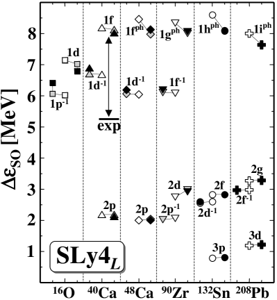
Figure 2: Neutron SO splittings (26) calculated using the SLy4_L functional. White, gray, and black symbols mark bare, mass and shape polarized (time-even), and mass, shape, and spin polarized (time-even and time-odd) results, respectively. Results for hole (particle and particle-hole) orbitals are shifted to the left (right) with respect to the core (open symbols). A typical discrepancy with experiment is shown by the arrow in ⁴⁰Ca.

The impact of polarization effects on the SO splittings is indeed very small, particularly for the cases where both SO partners are of particle or hole type. Indeed, for these cases, the effect only exceptionally exceeds 200 keV, reflecting a cancellation of polarization effects exerted on the $j=\ell\pm 1/2$ partners. The smallness of polarization effects hardly allows for any systematic trends to be pinned down. Nevertheless, the self-consistent results show a weak but relatively clear tendency to slightly enlarge or diminish the splitting for hole or particle states, respectively.

The situation is clearer when the SO partners are of mixed particle ($j=\ell-1/2$) and hole ($j=\ell+1/2$) character. In these cases, the shape polarization tends to diminish the splitting quite systematically by about 400–500 keV. This behavior follows from naive deformed Nilsson model picture where the highest-$K$ members of the $j=\ell-1/2$ ($j=\ell+1/2$) multiplet slopes down (up) as a function of the oblate (prolate) deformation parameter. As discussed in the previous Section, the time-odd fields act in the opposite way, tending to slightly enlarge the gap. The net polarization effect does not seem to exceed about 300 keV. In these cases, however, we deal with large $\ell$ orbitals having also quite large SO splittings of the order of $\sim$8 MeV. Hence, the relative corrections due to polarization effects do not exceed about 4%, i.e., they are relatively small – much smaller than the effects of tensor terms discussed below and the discrepancy with data, which in Fig. 2 is indicated for the neutron 1f SO splitting in ⁴⁰Ca. These results legitimate the direct use of bare s.p. spectra in magic cores for further studies of the SO splittings, which considerably facilitates the calculations.

As already mentioned, empirical s.p. energies are essentially deduced from differences between binding energies of doubly-magic core and their odd-$A$ neighbors. Different authors, however, use also one-particle transfer data, apply phenomenological particle-vibration corrections and/or treat slightly differently fragmented levels. Hence, published compilations of the s.p. energies, and in turn the SO splittings, differ slightly from one another depending on the assumed strategy. The typical uncertainties in the empirical SO splittings can be inferred from Table 3, which summarizes the available data on the SO splittings based on three recent s.p. level compilations published in Refs. [Isa02w] ; [Oro96w] ; [Sch07a] .

Nucleus	orbitals	Ref. [Isa02w]	Ref. [Oro96w]	Ref. [Sch07a]
16O	$\nu 1p_{3/2}^{-1}-\nu 1p_{1/2}^{-1}$	6.17	6.18	$--$
	$\nu 1d_{5/2}-\nu 1d_{3/2}$	5.08	5.72	5.08
	$\pi 1p_{3/2}^{-1}-\pi 1p_{1/2}^{-1}$	6.32	6.32	$--$
	$\pi 1d_{5/2}-\pi 1d_{3/2}$	5.00	4.97	5.00
40Ca	$\nu 2p_{3/2}-\nu 2p_{1/2}$	2.00	2.00	1.54
	$\nu 1f_{7/2}-\nu 1f_{5/2}$	4.88	5.24	5.64
	$\nu 1d_{5/2}^{-1}-\nu 1d_{3/2}^{-1}$	6.00	6.75	6.75
	$\pi 2p_{3/2}-\pi 2p_{1/2}$	2.01	1.72	1.69
	$\pi 1f_{7/2}-\pi 1f_{5/2}$	4.95	5.41	6.05
	$\pi 1d_{5/2}^{-1}-\pi 1d_{3/2}^{-1}$	6.00	5.94	6.74
48Ca	$\nu 2p_{3/2}-\nu 2p_{1/2}$	$--$	1.67	1.77
	$\nu 1f_{7/2}^{-1}-\nu 1f_{5/2}$	$--$	8.01	8.80
	$\nu 1d_{5/2}^{-1}-\nu 1d_{3/2}^{-1}$	$--$	5.30	3.08
	$\pi 2p_{3/2}-\pi 2p_{1/2}$	$--$	2.14	1.77
	$\pi 1f_{7/2}-\pi 1f_{5/2}$	$--$	4.92	$--$
	$\pi 1d_{5/2}^{-1}-\pi 1d_{3/2}^{-1}$	$--$	5.01	5.29
56Ni	$\nu 2p_{3/2}-\nu 2p_{1/2}$	$--$	1.88	1.12
	$\nu 1f_{7/2}^{-1}-\nu 1f_{5/2}$	$--$	6.82	7.16
	$\pi 2p_{3/2}-\pi 2p_{1/2}$	$--$	1.83	1.11
	$\pi 1f_{7/2}^{-1}-\pi 1f_{5/2}$	$--$	7.01	7.50
90Zr	$\nu 2d_{5/2}-\nu 2d_{3/2}$	$--$	2.43	$--$
	$\nu 1g_{9/2}^{-1}-\nu 1g_{7/2}$	$--$	7.07	$--$
	$\nu 2p_{3/2}^{-1}-\nu 2p_{1/2}^{-1}$	$--$	0.37	$--$
	$\nu 1f_{7/2}^{-1}-\nu 1f_{5/2}^{-1}$	$--$	1.71	$--$
	$\pi 2d_{5/2}-\pi 2d_{3/2}$	$--$	2.03	$--$
	$\pi 1g_{9/2}-\pi 1g_{7/2}$	$--$	5.56	$--$
	$\pi 2p_{3/2}^{-1}-\pi 2p_{1/2}^{-1}$	$--$	1.50	$--$
	$\pi 1f_{7/2}^{-1}-\pi 1f_{5/2}^{-1}$	$--$	4.56	$--$
100Sn	$\nu 2d_{5/2}-\nu 2d_{3/2}$	1.93	$--$	1.93
	$\nu 1g_{9/2}^{-1}-\nu 1g_{7/2}$	7.00	$--$	7.00
	$\pi 1g_{9/2}^{-1}-\pi 1g_{7/2}$	6.82	$--$	6.82
	$\pi 2p_{3/2}^{-1}-\pi 2p_{3/2}^{-1}$	2.85	$--$	2.85
132Sn	$\nu 2f_{7/2}-\nu 2f_{5/2}$	2.00	1.94	$--$
	$\nu 3p_{3/2}-\nu 3p_{1/2}$	0.81	0.59	1.15
	$\nu 1h_{11/2}^{-1}-\nu 1h_{9/2}$	6.53	6.51	6.68
	$\nu 2d_{5/2}^{-1}-\nu 2d_{3/2}^{-1}$	1.65	1.93	1.66
	$\pi 2d_{5/2}-\pi 2d_{3/2}$	1.48	1.83	1.75
	$\pi 1g_{9/2}^{-1}-\pi 1g_{7/2}$	6.08	5.33	6.08
208Pb	$\nu 3d_{5/2}-\nu 3d_{3/2}$	0.97	0.89	0.97
	$\nu 2g_{9/2}-\nu 2g_{7/2}$	2.50	2.38	2.50
	$\nu 1i_{13/2}^{-1}-\nu 11_{11/2}$	5.84	5.81	6.08
	$\nu 3p_{3/2}^{-1}-\nu 3p_{1/2}^{-1}$	0.90	0.90	0.89
	$\nu 2f_{7/2}^{-1}-\nu 2f_{5/2}^{-1}$	2.13	2.18	1.87
	$\pi 2f_{7/2}-\pi 2f_{5/2}$	1.93	2.02	1.93
	$\pi 3p_{3/2}-\pi 3p_{1/2}$	0.85	0.45	0.52
	$\pi 1h_{11/2}^{-1}-\pi 1h_{9/2}$	5.56	5.03	5.56
	$\pi 2d_{5/2}^{-1}-\pi 2d_{3/2}^{-1}$	1.68	1.62	1.46

Table 3: Empirical SO splittings. Compilation is based on the empirical s.p. levels taken from Refs. [Isa02w] ; [Oro96w] ; [Sch07a] .

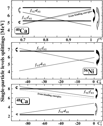
Figure 3: Figure illustrates the three-step procedure used to fit the isoscalar SO coupling constant $C^{\nabla J}_{0}$ in ⁴⁰Ca (upper panel), the isoscalar tensor strength $C_{0}^{J}$ in ⁵⁶Ni (middle panel), and the isovector tensor strength $C_{1}^{J}$ in ⁴⁸Ca (lowest panel). These particular calculations have been done for the SkP functional, but the pattern is common for all the analyzed parameterizations including SLy4 and SkO. See text for further details.

Instead of large-scale fit to the data (see, e.g., Refs. [Bri07w] ; [Les07] ), we propose a simple three-step method to adjust three coupling constants $C_{0}^{\nabla J}$, $C_{0}^{J}$, and $C_{1}^{J}$. The entire idea of this procedure is based on the observation that the empirical $1f_{7/2}-1f_{5/2}$ SO splittings in ⁴⁰Ca, ⁵⁶Ni, and ⁴⁸Ca form very distinct pattern, which cannot be reproduced by using solely the conventional SO interaction.

The readjustment is done in the following way. First, experimental data in the spin-saturated (SS) nucleus ⁴⁰Ca are used in order to fit the isoscalar SO coupling constant $C^{\nabla J}_{0}$. One should note that in this nucleus, the SO splitting depends only on $C^{\nabla J}_{0}$, and not on $C^{J}_{0}$ (because of the spin saturation), nor on $C^{\nabla J}_{1}$ (because of the isospin invariance at $N=Z$), nor on $C^{J}_{1}$ (because of both reasons above). Therefore, here one experimental number determines one particular coupling constants.

Second, once $C^{\nabla J}_{0}$ is fixed, the spin-unsaturated (SUS) $N=Z$ nucleus ⁵⁶Ni is used to establish the isoscalar tensor coupling constant $C_{0}^{J}$. Again here, because of the isospin invariance, the SO splitting is independent of either of the two isovector coupling constants, $C^{\nabla J}_{1}$ or $C^{J}_{1}$. Finally, in the third step, ⁴⁸Ca is used to adjust the isovector tensor coupling constant $C_{1}^{J}$. Such a procedure exemplifies the focus of fit on the s.p. properties, as discussed in the Introduction.

It turns out that current experimental data, and in particular lack of information in ⁴⁸Ni, do not allow for adjusting the fourth coupling constant, $C^{\nabla J}_{1}$. For this reason, in the present study we fix it by keeping the ratio of $C^{\nabla J}_{0}/C^{\nabla J}_{1}$ equal to that of the given standard Skyrme force. In the process of fitting, all the remaining time-even coupling constants $C_{t}$ are kept unchanged. Variants of the standard functionals obtained in this way are below denoted by SkP_T, SLy4_T, and SkO_T. When the time-odd channels, modified so as to reproduce the Landau parameters, are active, we also use notation SkP_LT, SLy4_LT, and SkO_LT.

For the SkP functional, the procedure is illustrated in Fig. 3. We start with the isoscalar $N=Z$ nucleus ⁴⁰Ca. The evolution of the SO splittings in function of $f^{\nabla J}$, which is the factor scaling the original SkP coupling constant $C_{0}^{\nabla J}$, is shown in the upper panel of Fig. 3. As it is clearly seen from the Figure, fair agreement with data requires about 20% reduction in the conventional SO interaction strength $C_{0}^{\nabla J}$. It should be noted also that the reduction in the SO interaction considerably improves the $1f_{7/2}-1d_{3/2}$ and $1f_{7/2}-2p_{3/2}$ splittings but slightly spoils the $2p_{3/2}-2p_{1/2}$ SO splitting. Qualitatively, similar results were obtained for the SLy4 and SkO interactions. Reasonable agreement to the data requires $\sim$20% reduction of the original $C_{0}^{\nabla J}$ in case of the SkO interaction and quite drastic $\sim$35% reduction of the original $C_{0}^{\nabla J}$ in case of the SLy4 force.

Having fixed $C_{0}^{\nabla J}$ in ⁴⁰Ca we move to the isoscalar nucleus ⁵⁶Ni. This nucleus is spin-unsaturated and therefore is very sensitive to the isoscalar $C_{0}^{J}$ tensor coupling constant. The evolution of theoretical s.p. levels versus $C_{0}^{J}$ is illustrated in the middle panel of Fig. 3. As shown in the Figure, reasonable agreement between the empirical and theoretical $1f_{7/2}-1f_{5/2}$ SO splitting is achieved for $C_{0}^{J}\sim-40$ MeV fm⁵, which by a factor of about five exceeds the original SkP value for this coupling constant. It is striking that a similar value of $C_{0}^{J}$ is obtained in the analogical analysis performed for the SLy4 interaction.

Finally, the isovector tensor coupling constant $C_{1}^{\nabla J}$ is established in $N$$\neq$$Z$ nucleus ⁴⁸Ca. The evolution of theoretical neutron s.p. levels versus $C_{1}^{J}$ is illustrated in the lowest panel of Fig. 3. As shown in the Figure, the value of $C_{1}^{\nabla J}\sim-70$ MeV fm⁵ is needed to reach reasonable agreement for the $1\nu f_{7/2}-1\nu f_{5/2}$ SO splitting in this case. For this value of the $C_{1}^{J}$ strength one obtains also good agreement for the proton $1\pi f_{7/2}-1\pi f_{5/2}$ SO splitting (see Figs. 4 and 5 below), without any further readjustment of the $C_{1}^{\nabla J}$ strength. Again, very similar value for the $C_{1}^{J}$ strength is deduced for the SLy4 force. Note also the improvement in the $1f_{7/2}-1d_{3/2}$ splitting caused by the isovector tensor interaction. Dotted lines show results obtained from the mass differences, i.e., with all the polarization effects included.

During the fitting procedure all the remaining functional coupling constants were kept fixed at their Skyrme values. The ratio of the isoscalar to the isovector coupling constant in the SO interaction channel was locked to its standard Skyrme value of $C_{0}^{\nabla J}/C_{1}^{\nabla J}=3$. Since no clear indication for relaxing this condition is seen (see also Figs. 4 and 5 below), we have decided to investigate the isovector degree of freedom in the SO interaction (see [Rei95] ) by performing our three-step fitting process also for the generalized Skyrme interaction SkO [Rei99fw] , for which $C_{0}^{\nabla J}/C_{1}^{\nabla J}\sim-0.78$.

Skyrme	$C_{0}^{\nabla J}$	$C_{0}^{\nabla J}/C_{1}^{\nabla J}$	$C_{0}^{J}$	$C_{1}^{J}$
force	[MeV fm5]		[MeV fm5]	[MeV fm5]
SkPT	$-$60.0	3	$-$38.6	$-$61.7
SLy4T	$-$60.0	3	$-$45.0	$-$60.0
SkOT	$-$61.8	$-$0.78	$-$33.1	$-$91.6

Table 4: Spin-orbit $C^{\nabla J}$ and tensor isoscalar $C_{0}^{J}$ and isovector $C_{1}^{J}$ functional coupling constants adopted in this work and subsequently used in Figs. 4, 5, and 6, where global calculations of the SO splittings are presented.

All the adopted functional coupling constants resulting from our calculations are collected in Table 4. Note, that the procedure leads to essentially identical SO interaction strengths $C_{0}^{\nabla J}$ for all three forces irrespective of their intrinsic differences, for example in effective masses. The tensor coupling constants in both the SkP and the SLy4 functionals are also very similar. In the SkO case, one observes rather clear enhancement in the isovector tensor coupling constant which becomes more negative to, most likely, counterbalance the non-standard positive strength in the isovector SO channel.

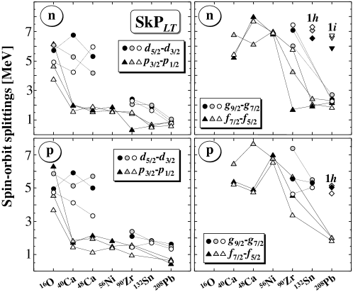
Figure 4: Experimental [Oro96w] (black symbols) and theoretical SO splittings calculated using the original SkP functional (gray symbols) and our modified SkP_LT functional (white symbols) with the SO and tensor coupling constants given in Table 4. Upper left and right panels show neutron SO splittings for low-$\ell=1,2$ ($p$ and $d$) and high-$\ell\geq 3$ orbitals, respectively. Analogical information but for proton SO splittings is depicted in the lower panels.

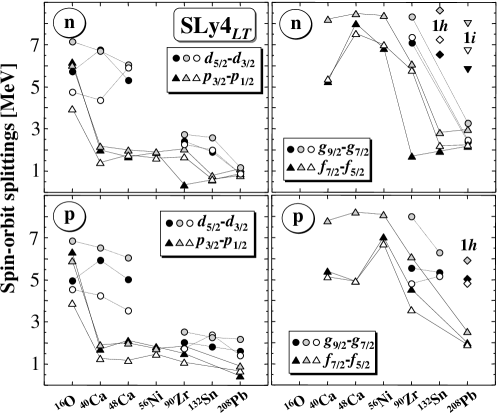
Figure 5: Same as in Fig. 4 but for the SLy4 functional.

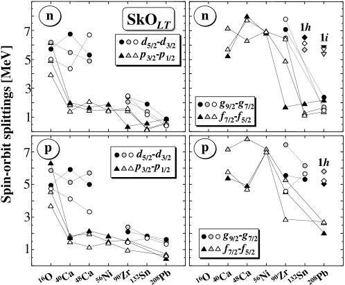
Figure 6: Same as in Fig. 4 but for the SkO functional.

The functionals were modified using only three specific pieces of data on the neutron $1f_{7/2}-1f_{5/2}$ SO splittings. In order to verify the reliability of the modifications, we have performed systematic calculations of the experimentally accessible SO splittings. The results are depicted in Figs. 4, 5, and 6 for the SkP, SLy4, and SkO functionals, respectively. Additionally, Fig. 7 shows neutron and proton magic gaps (III) calculated using the SkP functional. In all these Figures, estimates taken from Ref. [Oro96w] are used as reference empirical data.

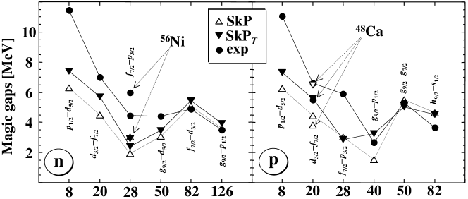
Figure 7: Experimental [Oro96w] (dots) and theoretical values of magic gaps (III), calculated using the original SkP functional (open triangles) and the SkP_T functional (full triangles) with the SO and the tensor coupling constants from Table. 4. The gaps were computed using the bare unpolarized s.p. spectra.

This global set of the results can be summarized as follows:

• The $\ell=1$, $p_{3/2}-p_{1/2}$, SO splittings are slightly better reproduced with original rather than modified functionals.

• The $1d$ SO splittings (¹⁶O, ^40,48Ca) are rather poorly reproduced by both the original and modified functionals. These splitting are also subject to relatively big empirical uncertainties as shown in Table 3 and, therefore, need not be very conclusive. In particular, the $1d$ SO splittings in $N$=$Z$ ¹⁶O and ⁴⁰Ca nuclei deduced from Ref. [Oro96w] and depicted in the figures show surprisingly large isospin dependence.

• The $2d$ and $3d$ splittings are quite well reproduced by both the original and modified functionals with slight preference for the modified functional, in particular for the SLy4 interaction.

• All the $\ell\geq 3$ SO splittings are reproduced considerably better by the modified functionals.

• Magic gaps are also better (although not fully satisfactorily) reproduced by the modified functionals.

Without any doubt the SO splittings are better described by the modified functionals. It should be stressed that the improvements were reached using only three additional data points without any further optimization. The tensor coupling constants deduced in this work and collected in table 4 should be therefore considered as reference values. Indeed, direct calculations show that variations in $C_{t}^{J}$ within $\pm$10% affect the calculated SO splittings only very weakly. The price paid for the improvements concerns mostly the binding energies, which for the nuclei ⁵⁶Ni, ¹³²Sn, and ²⁰⁸Pb become worse as compared to the original values. This issue is addressed in the next section.

V Binding energies

Parameters of the Skyrme functional have been fitted to reproduce several physical quantities, with emphasis on the masses of magic nuclei. Therefore it is not surprising that dramatic modifications of the SO and tensor terms of the functional, described in Sec. III, while improving the agreement between the calculated and measured single-particle properties, can destroy the quality of the mass fit. Hence, it is interesting to know whether this disagreement is significant and whether it can be healed by refitting the remaining parameters of the functional.

Table 5 shows differences between calculated and experimental (Ref. [Aud03] ) ground-state energies, $E_{\mathrm{calc}}-E_{\mathrm{exp}}$, (in MeV) for a set of spherical nuclei. Negative values mean that nuclei are overbound. Results given in the second column, denoted as SLy4, correspond to the standard SLy4 [Cha97fw] parametrization. The third column, denoted as SLy4_T, illustrates significant deterioration of the quality of fit when parameters $C^{\nabla J}_{0}$, $C_{0}^{J}$ and $C_{1}^{J}$ are modified (see Sec. III). Values presented in the last column, SLy4_Tmin, were obtained by minimizing the rms of relative discrepancies between the calculated and measured masses Values of $C^{\nabla J}_{0}$, $C_{0}^{J}$ and $C_{1}^{J}$ were kept fixed at their SLy4_T values, while minimization was performed by varying the remaining parameters of the functional $t_{i}$ and $x_{i}$. Note that for the standard SLy4 functional, the tensor coupling constants are set equal to zero independently of the values of $t_{i}$ and $x_{i}$. For the minimization, we have used the same methodology, namely, the influence of parameters $t_{i}$ and $x_{i}$ on tensor coupling constants was disregarded.

It should be emphasized that no attempt has been made to find the global minimum — the minimization was purely local, in the vicinity of the standard SLy4 values of the parameters $t_{i}$ and $x_{i}$. One can see that even this very limited procedure can lead to significant reduction of discrepancies, down to quite reasonable values (with an exception of ⁵⁶Ni nucleus).

Nucleus	SLy4	SLy4T	SLy4Tmin
40Ca	$-$2.197	$-$1.830	$-$5.775
48Ca	$-$1.912	5.039	$-$0.279
56Ni	0.625	15.138	9.127
90Zr	$-$1.845	7.492	$-$3.032
132Sn	$-$0.660	19.898	2.222
208Pb	0.822	24.910	$-$3.048

Table 5: Differences between calculated and experimental ground-state energies, $E_{\mathrm{calc}}-E_{\mathrm{exp}}$, (in MeV) for a set of spherical nuclei. Column denoted as SLy4_Tmin shows results obtained after (local) minimization with respect to parameters $t_{i},x_{i},\,i=0,1,2,3$. See text for details.

It is worth noting that the resulting modifications of the $t_{i}$ and $x_{i}$ parameters turned out to be very small. Table 6 shows the values of the $t_{i}$ and $x_{i}$ parameters in the standard SLy4 parametrization (second column) and those obtained as the result of the minimization procedure (third column). The last column shows relative changes of parameters (in percent). As one can see, they are at most of the order of one percent. Nevertheless, even such small changes were sufficient to improve significantly the agreement between calculated and experimental masses.

We stress again that the refitting procedure is used here only for illustration purposes and the global fit to masses must probably include extended functionals and improved methodology. For example, the Wigner energy correction [Wig37] was not included in the fit, as it was neither included in the fit of the SLy4 parametrization. This correction alone may change the balance of discrepancies obtained for the $N=Z$ and $N\neq Z$ nuclei, and strongly impact the results. Systematic studies of these effects will be performed in the near future.

param.	SLy4	SLy4Tmin	change (%)
$t_{0}$	$-$2488.913	$-$2490.00300	0.04
$t_{1}$	486.818	486.78460	$-$0.01
$t_{2}$	$-$546.395	$-$545.35849	$-$0.19
$t_{3}$	13777.000	13767.77776	$-$0.07
$x_{0}$	0.834	0.83257	$-$0.17
$x_{1}$	$-$0.344	$-$0.34227	$-$0.50
$x_{2}$	$-$1.000	$-$0.99798	$-$0.20
$x_{3}$	1.354	1.36128	0.54

Table 6: Skyrme force parameters $t_{i},x_{i},\,i=0,1,2,3$ of the standard SLy4 parametrization (second column) compared with those obtained from the minimization procedure described in the text (third column). The last column shows relative change of parameters (in percent).

VI Conclusions

Applicability of functional-based self-consistent mean-field or energy-density-functional methods to nuclear structure is hampered by their unsatisfactory s.p. properties. This fact seems to be a mere consequence of strategies used to select datasets that were applied in the process of adjusting free parameters of these effective theories. In spite of the fact that the s.p. energies are at the heart of these methods, the datasets are heavily oriented towards reproducing bulk nuclear properties in large-$N$ limit, with only a marginal influence of the s.p. levels or level splittings in finite nuclei.

In this work we suggest a necessity of shifting attention from bulk to s.p. properties and to look for spectroscopic-quality EDF, even at the expense of deteriorating its quality in reproducing binding energies. Such a strategy requires well-defined empirical input related to the s.p. energies, to be used directly in the fitting process. We argue that odd-even mass differences around magic nuclei not only provide unambiguous direct information about nuclear s.p. energies but are also well anchored within the spirit of the EDF formalism. Indeed, the theorems due to Hochenberg and Kohn [Hoh64w] and Levy [Lev76] , see also Refs. [Gir07] , imply existence of universal EDF capable, at least in principle, treating ground-states energies of nuclei exactly. One can, therefore, argue that this implies essentially exact treatment of at least the lowest s.p. levels forming ground states in one-particle (one-hole) odd-$A$ nuclei with respect to even-even cores or, alternatively, almost exact description of core-polarization phenomena caused by odd single-particle (single-hole).

An attempt to refit the EDF is preceded by a systematic analysis of the s.p. energies and self-consistent core-polarization effects within the state-of-the-art Skyrme-force-inspired EDF. Three major sources of core-polarization, including mass, shape and spin (time-odd) effects, are identified and discussed. The analysis is performed for even-even doubly-magic cores and the lowest s.p. states in odd-$A$ one-particle(hole) nuclei. The discussion is supplemented by analysis of the s.p. SO splittings.

New strategy in fitting the EDF is applied to the SO and tensor parts of the nuclear EDF. Instead of large-scale fit to binding energies we propose simple and intuitive three-step procedure that can be used to fit the isoscalar strength of the SO interaction as well as the isoscalar and isovector strengths of the tensor interaction. The entire idea is based on the observation that the $f_{7/2}-f_{5/2}$ SO splittings in spin-saturated isoscalar ⁴⁰Ca, spin-unsaturated isoscalar ⁵⁶Ni, and spin-unsaturated isovector ⁴⁸Ca form distinct pattern that can neither be understood nor reproduced based solely on the conventional SO interaction. The procedure indicates a clear need for major reduction (from $\sim$20% till $\sim$35% depending on the parameterization) of the SO strength and for strong tensor fields. It is verified that the suggested changes lead to systematic improvements of the functional performance concerning such s.p. properties like the SO splittings or magic gaps. It is also shown that destructive impact of these changes on the binding energies can be improved, to a large extent, by relatively small refinements of the remaining coupling constants.

This work was supported in part by the Polish Ministry of Science and by the Academy of Finland and University of Jyväskylä within the FIDIPRO programme.

References

- (1) P. Ring and P. Schuck, The Nuclear Many-Body Problem (Springer-Verlag, Berlin, 1980).
- (2) D. Lunney, J. M. Pearson, and C. Thibault Rev. Mod. Phys. 75, 1021 (2003).
- (3) M. Bender, P.-H. Heenen, and P.-G. Reinhard, Rev. Mod. Phys. 75, 121 (2003).
- (4) K. Rutz, M. Bender, J.A. Maruhn, P.-G. Reinhard, W. Greiner, Nucl. Phys. A634, 67 (1998).
- (5) I. Hamamoto and P. Siemens, Nucl. Phys. A269, 199 (1976).
- (6) V. Bernard and N. Van Giai, Nucl. Phys. A348, 75 (1980).
- (7) V.I. Isakov, K.I. Erokhina, H. Mach, M. Sanchez-Vega, and B. Fogelberg, Eur. Phys. J. A14, 29 (2002).
- (8) A. Oros, Ph.D. thesis, University of Köln, 1996.
- (9) N. Schwierz, I. Wiedenhover, and A. Volya, arXiv:0709.3525.
- (10) J. Dobaczewski and J. Dudek, Phys. Rev. C52, 1827 (1995); C55, 3177(E) (1997).
- (11) E. Perlińska, S.G. Rohoziński, J. Dobaczewski, and W. Nazarewicz, Phys. Rev. C 69, 014316 (2004).
- (12) Y.M. Engel, D.M. Brink, K. Goeke, S.J. Krieger, and D. Vautherin, Nucl. Phys. A 249, 215 (1975).
- (13) H. Flocard, Thesis 1975, Orsay, Série A, N∘ 1543.
- (14) Fl. Stancu, D.M. Brink, H. Flocard, Phys. Lett. 68B, 108 (1977).
- (15) J. Dobaczewski, Proc. of the 3rd ANL/MSU/INT/JINA RIA Theory Workshop, Argonne, USA, April 4-7, 2006, nucl-th/0604043.
- (16) T. Lesinski, M. Bender, K. Bennaceur, T. Duguet, and J. Meyer, Phys. Rev. C 76, 014312 (2007).
- (17) P.-G. Reinhard and H. Flocard, Nucl. Phys. A584, 467 (1995).
- (18) J. Dobaczewski, H. Flocard and J. Treiner, Nucl. Phys. A422, 103 (1984).
- (19) E. Chabanat, P. Bonche, P. Haensel, J. Meyer, and F. Schaeffer, Nucl. Phys. A627 (1997) 710; A635 (1998) 231.
- (20) P.-G. Reinhard, D.J. Dean, W. Nazarewicz, J. Dobaczewski, J.A. Maruhn, and M.R. Strayer, Phys. Rev. C60, 014316 (1999).
- (21) M. Bender, J. Dobaczewski, J. Engel, and W. Nazarewicz, Phys. Rev. C65, 054322 (2002).
- (22) H. Zduńczuk, W. Satuła, and R. Wyss, Phys. Rev. C71, 024305 (2005) ; Int. J. Mod. Phys. E14, 451 (2005) .
- (23) B. Fornal, S. Zhu, R.V.F. Janssens, M. Honma, R. Broda, P.F. Mantica, B.A. Brown, M.P. Carpenter, P.J. Daly, S.J. Freeman, Z.W. Grabowski, N.J. Hammond, F.G. Kondev, W. Krolas, T. Lauritsen, S.N. Liddick, C.J. Lister, E.F. Moore, T. Otsuka, T. Pawlat, D. Seweryniak, B.E. Tomlin, and J. Wrzesinski, Phys. Rev. C 70, 064304 (2004).
- (24) D.-C. Dinca, R.V.F. Janssens, A. Gade, D. Bazin, R. Broda, B.A. Brown, C.M. Campbell, M.P. Carpenter, P. Chowdhury, J.M. Cook, A.N. Deacon, B. Fornal, S.J. Freeman, T. Glasmacher, M. Honma, F.G. Kondev, J.-L. Lecouey, S.N. Liddick, P.F. Mantica, W.F. Mueller, H. Olliver, T. Otsuka, J.R. Terry, B.A. Tomlin, and K. Yoneda, Phys. Rev. C 71, 041302 (2005).
- (25) T. Otsuka, R. Fujimoto, Y. Utsuno, B.A. Brown, M. Honma, and T. Mizusaki, Phys. Rev. Lett. 87, 082502 (2001).
- (26) T. Otsuka, T. Suzuki, R. Fujimoto, H. Grawe, and Y. Akaish, Phys. Rev. Lett. 95, 232502 (2005).
- (27) M. Honma, T. Otsuka, B.A. Brown, and T. Mizusaki, Eur. Phys. Jour. 25,s01, 499 (2005).
- (28) T. Otsuka, T. Matsuo, and D. Abe, Phys. Rev. Lett. 97, 162501 (2006).
- (29) B.A. Brown, T. Duguet, T. Otsuka, D. Abe, and T. Suzuki, Phys. Rev. C 74, 061303(R) (2006).
- (30) J. Dobaczewski, N. Michel, W. Nazarewicz, M. Płoszajczak, and J. Rotureau, Prog. Part. Nucl. Phys. 59, 432 (2007).
- (31) D.M. Brink and Fl. Stancu, Phys. Rev. C75, 064311 (2007); nucl-th/0702065.
- (32) J. Dudek, Z. Szymański and T. Werner, Phys. Rev. C23, 920 (1981).
- (33) W. Nazarewicz, M.A. Riley, and J.D. Garrett, Nucl. Phys. A512, 61 (1990).
- (34) J.P. Jeukenne, A. Lejeunne, and C. Mahaux, Phys. Rev. C25, 83 (1976).
- (35) E. Litvinova and P. Ring, Phys. Rev. C73, 044328 (2006).
- (36) W. Satuła and R. Wyss, Phys. Lett. B572 (2003) 152; W. Satuła, R. Wyss, and M. Rafalski, Phys. Rev. C74, 011301(R) (2006).
- (37) T. Koopmans, Physica 1, 104 (1933).
- (38) M. Beiner, H. Flocard, N. Van Giai, and P. Quentin, Nucl. Phys. A 238, 29 (1975).
- (39) M. Bender, K. Rutz, P.-G. Reinhard, and J.A. Maruhn, Eur. Phys. Jour. A7, 467 (2000).
- (40) J. Skalski, Phys. Rev. C 74, 051601 (2006).
- (41) P. Olbratowski, J. Dobaczewski, and J. Dudek, Phys. Rev. C 73, 054308 (2006).
- (42) J. Dobaczewski and P. Olbratowski, Comput. Phys. Commun. 167, 214 (2005).
- (43) J. Dobaczewski, J. Dudek, and P. Olbratowski, HFODD User’s Guide: nucl-th/0501008 (2005).
-
(44)
J. Dobaczewski et al., HFODD home page:
http://www.fuw.edu.pl/~dobaczew/hfodd/. - (45) J. Dobaczewski, W. Satuła, J. Engel, P. Olbratowski, P. Powałowski, M. Sadziak, A. Staszczak, M. Zalewski, and H. Zduńczuk, Comput. Phys. Commun., to be published.
- (46) P. Finelli, N. Kaiser, D. Vretenar, and W. Weise, Nucl. Phys. A 791, 57 (2007).
- (47) G. Audi, A.H. Wapstra, and C. Thibault, Nucl. Phys. A729, 337 (2003).
- (48) E.P. Wigner, Phys. Rev. 51, 106 (1937).
- (49) P. Hohenberg and W. Kohn, Phys. Rev. 136, B864 (1964).
- (50) M. Levy, Proc. Natl. Acad. Sci USA 76, 6062 (1976).
- (51) B.G. Giraud, B.K. Jennings, and B.R. Barrett, arXiv:0707.3099 (2007); B.G. Giraud, arXiv:0707.3901 (2007).