Target Mass Corrections for the Virtual Photon Structure Functions to the Next-to-next-to-leading Order in QCD

Abstract

We investigate target mass effects in the unpolarized virtual photon structure functions $F_{2}^{\gamma}(x,Q^{2},P^{2})$ and $F_{L}^{\gamma}(x,Q^{2},P^{2})$ in perturbative QCD for the kinematical region $\Lambda^{2}\ll P^{2}\ll Q^{2}$, where $-Q^{2}(-P^{2})$ is the mass squared of the probe (target) photon and $\Lambda$ is the QCD scale parameter. We obtain the Nachtmann moments for the structure functions and then, by inverting the moments, we get the expressions in closed form for $F_{2}^{\gamma}(x,Q^{2},P^{2})$ up to the next-to-next-to-leading order and for $F_{L}^{\gamma}(x,Q^{2},P^{2})$ up to the next-to-leading order, both of which include the target mass corrections. Numerical analysis exhibits that target mass effects appear at large $x$ and become sizable near $x_{\rm max}(=1/(1+\frac{P^{2}}{Q^{2}}))$, the maximal value of $x$, as the ratio $P^{2}/Q^{2}$ increases.

I Introduction

It is well known that, in $e^{+}e^{-}$ collision experiments, the cross section for the two-photon processes $e^{+}e^{-}\rightarrow e^{+}e^{-}+{\rm hadrons}$ illustrated in Fig. 1 dominates at high energies over other processes such as one-photon annihilation process $e^{+}e^{-}\rightarrow\gamma^{*}\rightarrow{\rm hadrons}$. Here we consider the two-photon processes in the double-tag events, where both the outgoing $e^{+}$ and $e^{-}$ are detected. Especially, we investigate the case in which one of the virtual photon is far off-shell (large $Q^{2}\equiv-q^{2}$), while the other is close to the mass-shell (small $P^{2}=-p^{2}$). This process can be viewed as a deep-inelastic scattering off a photon target WalshBKT with mass squared $-P^{2}$, through which we can study the photon structure functions.

In the case of a real photon target ($P^{2}=0$), unpolarized (spin-averaged) photon structure functions $F_{2}^{\gamma}(x,Q^{2})$ and $F_{L}^{\gamma}(x,Q^{2})$ were studied first in the parton model WalshZerwas , and then investigated in perturbative QCD (pQCD). In the framework based on the operator product expansion (OPE) CHM supplemented by the renormalization (RG) group method, Witten Witten obtained the leading order (LO) QCD contributions to $F_{2}^{\gamma}$ and $F_{L}^{\gamma}$ and, shortly after, the next-to-leading order (NLO) QCD corrections to $F_{2}^{\gamma}$ were calculated by Bardeen and Buras BB . The same results were rederived by the QCD improved parton model approach Dewitt ; GR . The QCD analysis of the polarized photon structure function $g_{1}^{\gamma}(x,Q^{2})$ for the real photon target was performed in the LO KS and in the NLO SV ; GRS .

The structure functions $F_{2}^{\gamma}(x,Q^{2},P^{2})$ and $F_{L}^{\gamma}(x,Q^{2},P^{2})$ for the case of a virtual photon target ($P^{2}\neq 0$) were studied in the LO UW1 and in the NLO UW2 by pQCD. In fact, these structure functions were analyzed in the kinematical region,

$$\Lambda^{2}\ll P^{2}\ll Q^{2}~{},$$ (1)

where $\Lambda$ is the QCD scale parameter. The advantage of studying a virtual photon target in the kinematical region (1) is that we can calculate the whole structure function, its shape and magnitude, by the perturbative method. This is contrasted with the case of the real photon target where in the NLO there exist nonperturbative pieces. The virtual photon structure functions $F_{2}^{\gamma}$ and $F_{L}^{\gamma}$ were also studied by using the DGLAP-type QCD evolution equations Rossi ; DG ; GRStratmann ; Fontannaz . In the same kinematical region (1), the polarized virtual photon structure function $g_{1}^{\gamma}(x,Q^{2},P^{2})$ was investigated up to the NLO in QCD in Ref.SU1 and in the second paper of GRS . Moreover, the polarized parton distributions inside the virtual photon were analyzed in SU2 . Recently the first moment of $g_{1}^{\gamma}(x,Q^{2},P^{2})$ was calculated up to the next-to-next-to-leading order (NNLO) SUU . For more information on the recent theoretical and experimental investigation of unpolarized and polarized photon structure, see the review articles Krawczyk .

In our previous paper USU , we have studied the unpolarized virtual photon structure functions, $F_{2}^{\gamma}(x,Q^{2},P^{2})$ up to the NNLO and $F_{L}^{\gamma}(x,Q^{2},P^{2})$ up to the NLO, in pQCD for the kinematical region (1). This investigation became possible thanks to the recent three-loop calculations of the parton-parton as well as photon-parton splitting functions MVV1 ; MVV2 ; MVV3 . There we have considered the logarithmic corrections arising from the QCD higher-order effects up to the NNLO, and ignored all the power corrections of the form $(P^{2}/Q^{2})^{k}\ \ (k=1,2,\cdots)$ coming either from target mass effects or from higher-twist effects.

Figure 1: Deep inelastic scattering on a virtual photon in the $e^{+}~{}e^{-}$ collider experiments.

In fact, if the target is a real photon ($P^{2}=0$), there is no need to consider target mass corrections. But when the target becomes off-shell, for example, $P^{2}\geq M^{2}$, where $M$ is the nucleon mass, and for relatively low values of $Q^{2}$, contributions suppressed by powers of $P^{2}/Q^{2}$ may become important. Then we need to take into account these target mass contributions just like the case of the nucleon structure functions. The consideration of target mass effects (TME) is important by another reason. For the virtual photon target, the maximal value of the Bjorken variable $x$ is not 1 but

$$x_{\rm max}=\frac{1}{1+\frac{P^{2}}{Q^{2}}}~{},$$ (2)

due to the constraint $(p+q)^{2}\geq 0$, which is in contrast to the nucleon case where $x_{\rm max}=1$. The structure functions should vanish at $x=x_{\rm max}$. However, both the QCD NNLO result for $F_{2}^{\gamma}(x,Q^{2},P^{2})$ and the NLO result for $F_{L}^{\gamma}(x,Q^{2},P^{2})$ USU show that the predicted graphs do not vanish but remains finite at $x=x_{\rm max}$. This flaw is coming from the fact that TME have not been taken into account in the analysis. The target mass corrections have been studied in the past for the cases of unpolarized NACHT ; GP ; RGP and polarized WAND ; MU ; KU ; PR ; BK nucleon structure functions. As for the polarized virtual photon structure functions $g_{1}^{\gamma}(x,Q^{2},P^{2})$ and $g_{2}^{\gamma}(x,Q^{2},P^{2})$, TME have been studied in Ref. BSU .

In the present paper, we investigate the TME for the unpolarized virtual photon structure functions, $F_{2}^{\gamma}(x,Q^{2},P^{2})$ up to the NNLO and $F_{L}^{\gamma}(x,Q^{2},P^{2})$ up to the NLO, in pQCD. We use the framework of the OPE supplemented by the RG method. The photon matrix elements of the relevant traceless operators in the OPE are expressed by traceless tensors. These tensors contain many trace terms so that they satisfy the tracelessness conditions. The basic idea for computing the target mass corrections is to take account of these trace terms in the traceless tensors properly. There are two methods used so far for collecting all those trace terms. One, which was introduced by Nachtmann NACHT , is to make use of Gegenbauer polynomials to express the contractions between $q_{\mu_{1}}\cdots q_{\mu_{n}}$ and the traceless tensors NACHT ; WAND ; MU ; KU . This method leads to the Nachtmann moments for the operators with definite spin. The other, first used by Georgi and Politzer GP , is to write traceless tensors explicitly and then to collect trace terms and sum them up. Through the latter approach, the moments of structure functions are expressed as functions of the reduced operator matrix elements and coefficient functions with different spins. Actually both methods give equivalent results. In this paper we apply the former method to study the target mass corrections to the structure functions $F_{2}^{\gamma}$ and $F_{L}^{\gamma}$.

In the next section we discuss the framework for analyzing the TME based on the OPE. We introduce Gegenbauer polynomials to take account of the trace terms properly. In section 3 we derive the Nachtmann moments for the structure functions using the orthogonality relations of Gegenbauer polynomials. In section 4, by inverting the Nachtmann moments, we obtain the explicit expression for $F_{2}^{\gamma}(x,Q^{2},P^{2})$ (for $F_{L}^{\gamma}(x,Q^{2},P^{2})$) evaluated up to the NNLO (up to the NLO) with TME included. In section 5 we perform the numerical analysis and show that target mass corrections become sizable near $x_{\rm max}$. The final section is devoted to the conclusion.

II Operator Product Expansion

We analyze the virtual photon structure functions $F_{2}^{\gamma}(x,Q^{2},P^{2})$ and $F_{L}^{\gamma}(x,Q^{2},P^{2})$ using the theoretical framework based on the OPE and the RG method. Unless otherwise stated, we will follow the notation of Ref.BB .

Figure 2: Forward scattering of a virtual photon with momentum $q$ and another virtual photon with momentum $p$. The Lorentz indices are denoted by $\mu,\nu,\rho,\tau$.

Let us consider the forward virtual photon scattering amplitude for $\gamma(q)+\gamma(p)\rightarrow\gamma(q)+\gamma(p)$ illustrated in Fig.2,

$$T_{\mu\nu\rho\tau}(p,q)=i\int d^{4}xd^{4}yd^{4}ze^{iq\cdot x}e^{ip\cdot(y-z)}\langle 0|T(J_{\mu}(x)J_{\nu}(0)J_{\rho}(y)J_{\tau}(z))|0\rangle~{},$$ (3)

where $J_{\mu}$ is the electromagnetic current. Its absorptive part is related to the structure tensor $W_{\mu\nu\rho\tau}(p,q)$ for the target photon with mass squared $p^{2}=-P^{2}$ probed by the photon with $q^{2}=-Q^{2}$:

$$W_{\mu\nu\rho\tau}(p,q)=\frac{1}{\pi}{\rm Im}T_{\mu\nu\rho\tau}(p,q)~{}.$$ (4)

Taking a spin average for the target photon, we get

$$W_{\mu\nu}^{\gamma}(p,q) = \frac{1}{2}\sum_{\lambda}\epsilon^{\rho*}_{(\lambda)}(p)W_{\mu\nu\rho\tau}(p,q)\epsilon^{\tau}_{(\lambda)}(p)~{}$$ (5)

$$= -\frac{1}{2}g^{\rho\tau}W_{\mu\nu\rho\tau}(p,q)=\frac{1}{2}\int d^{4}xe^{iqx}\langle\gamma(p)|J_{\mu}(x)J_{\nu}(0)|\gamma(p)\rangle_{\rm spin\ av}.$$

Now $W_{\mu\nu}^{\gamma}(p,q)$ is expressed in terms of two independent structure functions $F_{L}^{\gamma}(x,Q^{2},P^{2})$ and $F_{2}^{\gamma}(x,Q^{2},P^{2})$ without neglecting the target mass squared $p^{2}$ (see Appendix A):

$$W_{\mu\nu}^{\gamma}(p,q) = e_{\mu\nu}\left\{\frac{1}{x}F_{L}^{\gamma}+\frac{p^{2}q^{2}}{(p\cdot q)^{2}}\frac{1}{x}F_{2}^{\gamma}\right\}+d_{\mu\nu}\frac{1}{x}F_{2}^{\gamma}~{},$$ (6)

where

$$e_{\mu\nu}=g_{\mu\nu}-\frac{q_{\mu}q_{\nu}}{q^{2}}$$ (7)

$$d_{\mu\nu}=-g_{\mu\nu}+\frac{p_{\mu}q_{\nu}+p_{\nu}q_{\mu}}{p\cdot q}-\frac{p_{\mu}p_{\nu}}{(p\cdot q)^{2}}q^{2}~{},$$ (8)

and $x$ is the Bjorken variable defined by $x=Q^{2}/2p\cdot q$.

Applying OPE for the product of two electromagnetic currents at short distance we get

$$i\int d^{4}xe^{iqx}T(J_{\mu}(x)J_{\nu}(0)) = \left(g_{\mu\nu}-\frac{q_{\mu}q_{\nu}}{q^{2}}\right)\sum_{n=0\atop n={\rm even}}\left(\frac{2}{Q^{2}}\right)^{n}q_{\mu_{1}}\cdots q_{\mu_{n}}\sum_{i}C^{i}_{L,n}O_{i}^{\mu_{1}\cdots\mu_{n}}$$ (9)

$$+ \Bigl{(}-g_{\mu\lambda}g_{\nu\sigma}q^{2}+g_{\mu\lambda}q_{\nu}q_{\sigma}+g_{\nu\sigma}q_{\mu}q_{\lambda}-g_{\mu\nu}q_{\lambda}q_{\sigma}\Bigr{)}$$

$$\times \sum_{n=2\atop n={\rm even}}\left(\frac{2}{Q^{2}}\right)^{n}q_{\mu_{1}}\cdots q_{\mu_{n-2}}\sum_{i}C^{i}_{2,n}O_{i}^{\lambda\sigma\mu_{1}\cdots\mu_{{n-2}}}+\cdots~{},$$

where $C^{i}_{L,n}$ and $C^{i}_{2,n}$ are the coefficient functions which contribute to the structure functions $F_{L}^{\gamma}$ and $F_{2}^{\gamma}$, respectively, and $O_{i}^{\mu_{1}\cdots\mu_{n}}$ and $O_{i}^{\lambda\sigma\mu_{1}\cdots\mu_{{n-2}}}$ are spin-$n$ twist-2 operators (hereafter we often refer to $O_{i}^{\mu_{1}\cdots\mu_{n}}$ as $O_{i}^{n}$). The sum on $i$ runs over the possible twist-2 operators and $\cdots$ represents other terms with irrelevant coefficient functions and operators. In fact, the relevant $O_{i}^{n}$ are flavor singlet quark ($\psi$), gluon ($G$), flavor nonsinglet quark ($NS$) and photon ($\gamma$) operators. It is noted that the operators $O_{i}^{n}$ are traceless and have totally symmetric Lorentz indices $\mu_{1}\cdots\mu_{n}$ ($\lambda\sigma\mu_{1}\cdots\mu_{n-2}$).

The spin-averaged matrix elements of these operators sandwiched by the photon states with momentum $p$ are expressed as

$$\langle\gamma(p)|O_{i}^{\mu_{1}\cdots\mu_{n}}|\gamma(p)\rangle_{\rm spin\ av} = A_{n}^{i}(\mu^{2},P^{2})~{}\{p^{\mu_{1}}\cdots p^{\mu_{n}}~{}-\ {\rm trace\ terms}\}$$ (10)

$$\equiv A_{n}^{i}(\mu^{2},P^{2})\{p^{\mu_{1}}\cdots p^{\mu_{n}}\}_{n}~{},$$

where $i=\psi,G,NS,\gamma$, and $A_{n}^{i}(\mu^{2},P^{2})$ is the reduced photon matrix element with $\mu$ being the renormalization point which we choose at $\mu^{2}=P^{2}$. For $-p^{2}=P^{2}\gg\Lambda^{2}$, we can calculate $A_{n}^{i}(P^{2})$ perturbatively. The $\{p^{\mu_{1}}\cdots p^{\mu_{n}}\}_{n}$ denotes the totally symmetric rank-$n$ tensor formed with the momentum $p$ alone and satisfies the traceless condition  $g_{\mu_{i}\mu_{j}}\{p^{\mu_{1}}\cdots p^{\mu_{n}}\}_{n}\!=\!0$ . Taking the spin-averaged photon matrix elements of (9) we obtain for the photon-photon forward-scattering amplitude

$$T_{\mu\nu}^{\gamma}(p,q) = i\int d^{4}xe^{iq\cdot x}\langle\gamma(p)|T(J_{\mu}(x)J_{\nu}(0))|\gamma(p)\rangle_{\rm spin\ av}$$ (11)

$$= \left(g_{\mu\nu}-\frac{q_{\mu}q_{\nu}}{q^{2}}\right)\sum_{n=0\atop n={\rm even}}\left(\frac{2}{Q^{2}}\right)^{n}q_{\mu_{1}}\cdots q_{\mu_{n}}\{p^{\mu_{1}}\cdots p^{\mu_{n}}\}_{n}~{}\sum_{i}C^{i}_{L,n}A_{n}^{i}(P^{2})$$

$$+ \Bigl{(}-g_{\mu\lambda}g_{\nu\sigma}q^{2}+g_{\mu\lambda}q_{\nu}q_{\sigma}+g_{\nu\sigma}q_{\mu}q_{\lambda}-g_{\mu\nu}q_{\lambda}q_{\sigma}\Bigr{)}$$

$$\times \sum_{n=2\atop n={\rm even}}\left(\frac{2}{Q^{2}}\right)^{n}q_{\mu_{1}}\cdots q_{\mu_{n-2}}\{p^{\lambda}p^{\sigma}p^{\mu_{1}}\cdots p^{\mu_{n-2}}\}_{n}\sum_{i}C^{i}_{2,n}A_{n}^{i}(P^{2})~{}.$$

The basic idea for treating target mass corrections exactly is to take account of trace terms in the traceless tensors properly. We evaluate the contraction between $q_{\mu_{1}}\cdots q_{\mu_{n}}$ and the traceless tensors without neglecting any of the trace terms. The results are expressed in terms of Gegenbauer polynomials NACHT ; WAND ; MU :

$$q_{\mu_{1}}\cdots q_{\mu_{n}}\{p^{\mu_{1}}\cdots p^{\mu_{n}}\}_{n}=a^{n}C_{n}^{(1)}(\eta)~{},$$ (12)

$$q_{\mu_{1}}\cdots q_{\mu_{n-2}}\{p^{\lambda}p^{\sigma}p^{\mu_{1}}\cdots p^{\mu_{n-2}}\}_{n}=\frac{1}{n(n-1)}\left[\frac{g^{\lambda\sigma}}{Q^{2}}a^{n}2C_{n-2}^{(2)}(\eta)+\frac{q^{\lambda}q^{\sigma}}{Q^{4}}a^{n}8C_{n-4}^{(3)}(\eta)\right.$$

$$\hskip 142.26378pt\left.+p^{\lambda}p^{\sigma}a^{n-2}2C_{n-2}^{(3)}(\eta)+\frac{p^{\lambda}q^{\sigma}+q^{\lambda}p^{\sigma}}{Q^{2}}a^{n-1}4C_{n-3}^{(3)}(\eta)\right],$$ (13)

where

$$a=-\frac{1}{2}PQ,\quad\eta=-\frac{p\cdot q}{PQ}~{},$$ (14)

and $C_{n}^{(\nu)}(\eta)$’s are Gegenbauer polynomials (see Appendix B). Recall that in the case of a nucleon target with mass $M$, we had $p^{2}=M^{2}$, $\eta=ip\cdot q/MQ$ and $a=-\frac{1}{2}iMQ$ WAND . In the photon case, we have $p^{2}=-P^{2}$ instead, and thus, replacing $M$ with $-iP$, we obtain the expressions for $a$ and $\eta$ in (14). The derivation of Eqs.(12) and (13) are given in Appendix C.

We decompose the amplitude $T_{\mu\nu}^{\gamma}(p,q)$ as

$$T_{\mu\nu}^{\gamma}(p,q)=e_{\mu\nu}\left\{\frac{1}{x}T_{L}^{\gamma}+\frac{p^{2}q^{2}}{(p\cdot q)^{2}}\frac{1}{x}(p\cdot q)T_{2}^{\gamma}\right\}+d_{\mu\nu}\frac{1}{x}(p\cdot q)T_{2}^{\gamma}~{},$$ (15)

then, using the results (12) and (13), we find from Eq.(11)

$$\frac{1}{x}(p\cdot q)T_{2}^{\gamma}=\sum_{n=2\atop n={\rm even}}\left(-\frac{P}{Q}\right)^{n}8\eta^{2}C_{n-2}^{(3)}(\eta)\frac{1}{n(n-1)}~{}M_{2,n}^{\gamma}~{},$$ (16)

$$\frac{1}{x}T_{L}^{\gamma}+\frac{p^{2}q^{2}}{(p\cdot q)^{2}}\frac{1}{x}(p\cdot q)T_{2}^{\gamma}=\sum_{n=0\atop n={\rm even}}\left(-\frac{P}{Q}\right)^{n}C_{n}^{(1)}(\eta)~{}M_{L,n}^{\gamma}$$

$$\qquad+\sum_{n=2\atop n={\rm even}}\left(-\frac{P}{Q}\right)^{n}\frac{4}{n(n-1)}\times\left[C_{n-2}^{(2)}(\eta)-2C_{n-4}^{(3)}(\eta)+4\eta C_{n-3}^{(3)}(\eta)\right]M_{2,n}^{\gamma}~{},$$ (17)

where we have defined

$$M_{2,n}^{\gamma}\equiv\frac{1}{2}\sum_{i}C^{i}_{2,n}(Q^{2},P^{2},g)A_{n}^{i}(P^{2}),\quad M_{L,n}^{\gamma}\equiv\frac{1}{2}\sum_{i}C^{i}_{L,n}(Q^{2},P^{2},g)A_{n}^{i}(P^{2})~{}.$$ (18)

III Nachtmann Moments

We derive the Nachtmann moments for the definite spin-$n$ contributions, $M_{2,n}^{\gamma}$ and $M_{L,n}^{\gamma}$. First we write the dispersion relations for $T_{2}^{\gamma}$ and $T_{L}^{\gamma}$, and we denote

$$F_{2}^{\gamma}=\frac{1}{\pi}{\rm Im}\ (p\cdot q)T_{2}^{\gamma},\qquad F_{L}^{\gamma}=\frac{1}{\pi}{\rm Im}T_{L}^{\gamma}~{}.$$ (19)

Then, using the orthogonality relation (66) and the integration formula (67) for the Gegenbauer polynomials $C_{n}^{(\nu)}(\eta)$, we can project out $M_{2,n}^{\gamma}$ and $M_{L,n}^{\gamma}$. The results are as follows:

$$\mu_{2,n}^{\gamma}(Q^{2},P^{2}) \equiv \int_{0}^{x_{\rm max}}dx\frac{1}{x^{3}}\xi^{n+1}\left[\frac{3+3(n+1)r+n(n+2)r^{2}}{(n+2)(n+3)}\right]F_{2}^{\gamma}(x,Q^{2},P^{2})=M_{2,n}^{\gamma},$$

$$\mu_{L,n}^{\gamma}(Q^{2},P^{2}) \equiv \int_{0}^{x_{\rm max}}dx\frac{1}{x^{3}}\xi^{n+1}\left[F_{L}^{\gamma}(x,Q^{2},P^{2})\right.$$ (21)

$$\hskip 34.14322pt+\left.\frac{4P^{2}x^{2}}{Q^{2}}\frac{(n+3)-(n+1)\xi^{2}P^{2}/Q^{2}}{(n+2)(n+3)}F_{2}^{\gamma}(x,Q^{2},P^{2})\right]=M_{L,n}^{\gamma}.$$

The Nachtmann moments $\mu_{2,n}^{\gamma}$ and $\mu_{L,n}^{\gamma}$ are given by the weighted integrals of the structure functions $F_{2}^{\gamma}$ and $F_{L}^{\gamma}$ and are equal to the definite spin-$n$ contributions, $M_{2,n}^{\gamma}$ and $M_{L,n}^{\gamma}$, respectively. The variables $r$ and $\xi$ are defined as

$$r\equiv\sqrt{1-\frac{4P^{2}x^{2}}{Q^{2}}}~{},\qquad\xi\equiv\frac{2x}{1+\sqrt{1-\frac{4P^{2}x^{2}}{Q^{2}}}}=\frac{2x}{1+r}.$$ (22)

We see from Eq.(2) that the maximal value of $x$ is not 1 but $1/[1+(P^{2}/Q^{2})]$. Therefore, the allowed ranges of $r$ and $\xi$ turn out to be $r_{\rm min}\leq r\leq 1$ and $0\leq\xi\leq 1$, respectively, where $r_{\rm min}=r(x_{\rm max})=(1-P^{2}/Q^{2})/(1+P^{2}/Q^{2})$ and $\xi(x_{\rm max})=1$.

We now outline how to derive the Nachtmann moments for the case of $F_{2}^{\gamma}(x,Q^{2},P^{2})$ given in (III). Since $(p\cdot q)/x=(-PQ\eta)(-P/Q)2\eta$, we see that $T_{2}^{\gamma}$ in (16) is expressed as

$$T_{2}^{\gamma}(x,Q^{2},P^{2})=\frac{1}{Q^{2}}\sum_{n=2\atop n={\rm even}}\left(-\frac{P}{Q}\right)^{n-2}\cdot 8C_{n-2}^{(3)}(\eta)\frac{1}{n(n-1)}M_{2,n}^{\gamma}~{}.$$ (23)

By the use of orthogonality relation of the Gegenbauer polynomials (66) for $\nu=3$ we get

$$\int_{-1}^{1}(1-\eta^{2})^{5/2}C_{n-2}^{(3)}(\eta)~{}T_{2}^{\gamma}d\eta=\frac{1}{Q^{2}}\frac{\pi}{2^{4}}\left(-\frac{P}{Q}\right)^{n-2}(n+2)(n+3)M_{2,n}^{\gamma}~{}.$$ (24)

Applying the dispersion relation, we can relate the full amplitude with its absorptive part:

$$T_{2}^{\gamma}(\omega)=\int_{\omega_{\rm min}}^{\infty}\left(\frac{1}{\omega^{\prime}-\omega}+\frac{1}{\omega^{\prime}+\omega}\right)W_{2}^{\gamma}(\omega^{\prime})d\omega^{\prime}~{},\quad\omega_{\rm min}=\frac{1}{x_{\rm min}}$$ (25)

where $\omega=2p\cdot q/Q^{2}=1/x$ and denoting $\zeta=(\omega^{\prime}Q)/(-2P)$, $\eta=(\omega Q)/(-2P)$ we derive

$$\int_{-1}^{1}(1-\eta^{2})^{5/2}C_{n-2}^{(3)}(\eta)T_{2}^{\gamma}d\eta=2\int_{\omega_{\rm min}}^{\infty}d\omega^{\prime}W_{2}^{\gamma}(\omega^{\prime},Q^{2},P^{2})\frac{Q}{(-2P)}\int_{-1}^{1}\frac{(-1)}{(-\zeta)-\eta}(1-\eta^{2})^{5/2}C_{n-2}^{(3)}(\eta)d\eta~{},$$

where we have noted $C_{n-2}^{(3)}(-\eta)=C_{n-2}^{(3)}(\eta)$ for even $n$. From (67) for $m=0$, $\nu=3$, we get

$$\int_{-1}^{1}(1-\eta^{2})^{5/2}C_{n-2}^{(3)}(\eta)T_{2}^{\gamma}d\eta$$

$$=\left(\frac{-Q}{2P}\right)\cdot\frac{\pi}{4}\cdot\int_{\omega_{\rm min}}^{\infty}d\omega W_{2}^{\gamma}(\omega,Q^{2},P^{2})\left(\zeta^{2}-1\right)(-1)\left[-\zeta-(\zeta^{2}-1)^{1/2}\right]^{n+1}(n+2)(n+3)$$

$$\hskip 85.35826pt\times\left[1-\frac{6}{n+2}z+\frac{12}{(n+2)(n+3)}z^{2}\right]~{},$$ (27)

where we used the following relation for the hypergeometric function with $\zeta=-p\cdot q/PQ$,

$$F(3,-2;n+2;z)=1-\frac{6}{n+2}z+\frac{12}{(n+2)(n+3)}z^{2},\quad z\equiv\frac{-(-\zeta)+(\zeta^{2}-1)^{1/2}}{2(\zeta^{2}-1)^{1/2}}~{},$$ (28)

Setting (24) equal to (27) and changing integration variable from $\omega$ to $x$, we get

$$\int_{0}^{x_{\rm max}}dx\frac{1}{x^{3}}\xi^{n+1}\left(1-\frac{4P^{2}x^{2}}{Q^{2}}\right)\left[1-\frac{6}{n+2}z+\frac{12}{(n+2)(n+3)}z^{2}\right]F_{2}^{\gamma}(x,Q^{2},P^{2})=M_{2,n}^{\gamma}~{}.$$

Here one should note that $n$ is even and the following relations hold:

$$-\zeta=\frac{Q}{2Px},\quad-\zeta-(\zeta^{2}-1)^{1/2}=\frac{P}{Q}\xi,\quad z=-\frac{P^{2}}{Q^{2}}\frac{\xi x}{r},\quad\xi=\frac{Q^{2}}{2P^{2}x}(1-r)~{},$$ (30)

and so we finally get for $F_{2}^{\gamma}(x,Q^{2},P^{2})$ as

$$\int_{0}^{x_{\rm max}}dx\frac{1}{x^{3}}\xi^{n+1}\left[\frac{3+3(n+1)r+n(n+2)r^{2}}{(n+2)(n+3)}\right]F_{2}^{\gamma}(x,Q^{2},P^{2})=M_{2,n}^{\gamma}(Q^{2},P^{2})~{},$$ (31)

where the left-hand side is $\mu_{2,n}^{\gamma}(Q^{2},P^{2})$, the Nachtmann moment, which is equal to the definite spin-$n$ contribution $M_{2,n}^{\gamma}$, and this is consistent with the previous result for the case of nucleon target NACHT ; Simula ; SteffensMelnitchouk ; Schi with a replacement of the variable $M\rightarrow-iP$.

For the longitudinal structure function, we first solve for $\frac{1}{x}T_{L}^{\gamma}$ from Eqs.(16) and (17) and we get (see Appendix B)

$$\frac{1}{x}T_{L}^{\gamma} = \sum_{n=0\atop n={\rm even}}\left(-\frac{P}{Q}\right)^{n}C_{n}^{(1)}(\eta)~{}M_{L,n}^{\gamma}$$ (32)

$$\quad+\sum_{n=2\atop n={\rm even}}\left(-\frac{P}{Q}\right)^{n}\frac{4}{n(n-1)}\left[\frac{-2}{n}C_{n-2}^{(3)}(\eta)+\frac{2}{n}C_{n-4}^{(3)}(\eta)\right]M_{2,n}^{\gamma}~{}.$$

Then using the recursion relation (72) for the case $\nu=1$:

$$C_{n}^{(1)}(\eta)=\frac{2}{(n+1)(n+2)}C_{n}^{(3)}(\eta)-\frac{4}{n(n+2)}C_{n-2}^{(3)}(\eta)+\frac{2}{n(n+1)}C_{n-4}^{(3)}(\eta)~{},$$ (33)

and the orthogonality relation of the Gegenbauer polynomials $C_{n}^{(3)}$’s we can derive the recursive relations for the sequence $M_{L,n}^{\gamma}$’s which can be solved as (See Appendix D):

$$\int_{0}^{x_{\rm max}}dx\frac{1}{x^{3}}\xi^{n+1}\left[F_{L}^{\gamma}(x,Q^{2},P^{2})+\frac{4P^{2}x^{2}}{Q^{2}}\frac{(n+3)-(n+1)\xi^{2}P^{2}/Q^{2}}{(n+2)(n+3)}F_{2}^{\gamma}(x,Q^{2},P^{2})\right]=M_{L,n}^{\gamma}~{},$$

where the left-hand side integral is the Nachtmann moment $\mu_{L,n}^{\gamma}$ for the longitudinal part. This coincides with the result obtained in NACHT ; Simula after the replacement mentioned above.

IV Inverting the Nachtmann Moments

We now invert the Nachtmann moments to express the structure functions $F_{2}^{\gamma}$ and $F_{L}^{\gamma}$ explicitly as functions of $x$, $Q^{2}$ and $P^{2}$. We first consider $F_{2}^{\gamma}$. By changing the integration variable from $x$ to $\xi$, we can rewrite the Nachtmann moments, given in Eqs.(III) and (21), as follows:

$$M_{2,n}^{\gamma} = \int_{0}^{1}d\xi\ \xi^{n-2}(1-\kappa\xi^{2})(1+\kappa\xi^{2})$$ (35)

$$\times\biggl{[}\frac{3}{(n+2)(n+3)}+\frac{3(n+1)}{(n+2)(n+3)}\frac{1-\kappa\xi^{2}}{1+\kappa\xi^{2}}+\frac{n}{n+3}\Bigl{(}\frac{1-\kappa\xi^{2}}{1+\kappa\xi^{2}}\Bigr{)}^{2}\biggr{]}~{}F_{2}^{\gamma}(x,Q^{2},P^{2})$$

$$M_{L,n}^{\gamma} = \int_{0}^{1}d\xi\ \xi^{n-2}(1-\kappa\xi^{2})(1+\kappa\xi^{2})$$ (36)

$$\times\biggl{[}F_{L}^{\gamma}(x,Q^{2},P^{2})+4\kappa\frac{\xi^{2}}{(1+\kappa\xi^{2})^{2}}\biggl{(}\frac{1}{n+2}-\kappa\xi^{2}\frac{n+1}{(n+2)(n+3)}\biggr{)}F_{2}^{\gamma}(x,Q^{2},P^{2})\biggr{]}~{}.$$

where we have made use of the following relations:

$$x=\frac{\xi}{1+\kappa\xi^{2}}~{},\quad r=\frac{1-\kappa\xi^{2}}{1+\kappa\xi^{2}}~{},\quad\frac{dx}{d\xi} = \frac{1-\kappa\xi^{2}}{(1+\kappa\xi^{2})^{2}}~{},$$ (37)

with $\kappa=P^{2}/Q^{2}$. Now we define

$$A(\xi)\equiv\frac{1-\kappa\xi^{2}}{1+\kappa\xi^{2}}~{}F_{2}^{\gamma}(x,Q^{2},P^{2})~{},\quad B(\xi)\equiv(1-\kappa\xi^{2})(1+\kappa\xi^{2})F_{L}^{\gamma}(x,Q^{2},P^{2})~{}.$$ (38)

Then the above two moments are written as

$$\frac{M_{2,n}^{\gamma}}{n(n-1)} = \int_{0}^{1}d\xi\ \xi^{n-2}\biggl{\{}\frac{A(\xi)}{n(n-1)}-\frac{2\kappa\xi^{2}~{}A(\xi)}{n(n+2)}+\frac{\kappa^{2}\xi^{4}~{}A(\xi)}{(n+2)(n+3)}\biggr{\}}$$ (39)

$$\frac{M_{L,n}^{\gamma}}{n+1} = \int_{0}^{1}d\xi\ \xi^{n-2}\biggl{\{}\frac{B(\xi)}{n+1}+\frac{4\kappa\xi^{2}~{}A(\xi)}{(n+1)(n+2)}-\frac{4\kappa^{2}\xi^{4}~{}A(\xi)}{(n+2)(n+3)}\biggr{\}}$$ (40)

The boundary conditions for $A(\xi)$ and $B(\xi)$ are $A(\xi=1)=B(\xi=1)=0$, since $F_{2}^{\gamma}(x_{\rm max},Q^{2},P^{2})=F_{L}^{\gamma}(x_{\rm max},Q^{2},P^{2})=0$ and $\xi(x_{\rm max})=1$. Now introducing the following four functions,

$$A_{0}(\xi)=\int^{1}_{\xi}d\xi^{\prime}~{}A(\xi^{\prime}),\quad A_{-1}(\xi) \equiv \int^{1}_{\xi}d\xi^{\prime}~{}\frac{A(\xi^{\prime})}{\xi^{\prime}},\quad A_{-2}(\xi)=\int^{1}_{\xi}d\xi^{\prime}~{}\frac{A(\xi^{\prime})}{{\xi^{\prime}}^{2}}$$ (41)

$$B_{-3}(\xi) \equiv \int^{1}_{\xi}d\xi^{\prime}~{}\frac{B(\xi^{\prime})}{{\xi^{\prime}}^{3}}$$ (42)

and by partial integration we find that the above two moments are written as

$$\frac{M_{2,n}^{\gamma}}{n(n-1)} = \int_{0}^{1}d\xi~{}\xi^{n-2}(1-\kappa\xi^{2})\Bigl{\{}(1+\kappa\xi^{2})A_{-1}(\xi)-\xi A_{-2}(\xi)-\kappa\xi A_{0}(\xi)\Bigr{\}},$$ (43)

$$\frac{M_{L,n}^{\gamma}}{n+1} = \int_{0}^{1}d\xi~{}\xi^{n}\Bigl{[}B_{-3}(\xi)+4\kappa\Bigl{\{}(1+\kappa\xi^{2})A_{-1}(\xi)-\xi A_{-2}(\xi)-\kappa\xi A_{0}(\xi)\Bigr{\}}\Bigr{]}.$$ (44)

Inverting the moments we get

$$G(\xi) = \frac{1}{2\pi i}\int_{c-i\infty}^{c+i\infty}dn\,\xi^{-n+1}\biggl{\{}\frac{M_{2,n}^{\gamma}}{n(n-1)}\biggr{\}}$$ (45)

$$= (1-\kappa\xi^{2})\Bigl{\{}(1+\kappa\xi^{2})A_{-1}(\xi)-\xi A_{-2}(\xi)-\kappa\xi A_{0}(\xi)\Bigr{\}},$$

$$S(\xi) = \frac{1}{2\pi i}\int_{c-i\infty}^{c+i\infty}dn\,\xi^{-n-1}\biggl{\{}\frac{M_{L,n}^{\gamma}}{n+1}\biggr{\}}$$ (46)

$$= B_{-3}(\xi)+\frac{4\kappa}{1-\kappa\xi^{2}}G(\xi),$$

where in Eq.(46) we have used the result of Eq.(45).

We further introduce the following functions,

$$H(\xi) \equiv -\frac{dG(\xi)}{d\xi}=\frac{1}{2\pi i}\int_{c-i\infty}^{c+i\infty}dn\,\xi^{-n}\frac{M_{2,n}^{\gamma}}{n}$$ (47)

$$F(\xi) \equiv -\frac{dH(\xi)}{d\xi}=\frac{1}{2\pi i}\int_{c-i\infty}^{c+i\infty}dn\,\xi^{-n-1}M_{2,n}^{\gamma}$$ (48)

$$F_{L}(\xi) \equiv -\xi\frac{dS(\xi)}{d\xi}=\frac{1}{2\pi i}\int_{c-i\infty}^{c+i\infty}dn\,\xi^{-n-1}M_{L,n}^{\gamma}~{}.$$ (49)

Differentiating both sides of Eqs.(45-46) with respect to $\xi$, we get the relations between ${A_{-1}}(\xi)$, $({A_{-2}}(\xi)+\kappa{A_{0}}(\xi))$, $A(\xi)$, $B(\xi)$ and $G(\xi)$, $H(\xi)$, $F_{2}(\xi)$ and $F_{L}(\xi)$. Now solving for $A(\xi)$ and $B(\xi)$ and, then recalling Eq.(38), we obtain

$$F_{2}^{\gamma}(x,Q^{2},P^{2}) = \frac{x^{2}}{r^{3}}F(\xi)-6\kappa\frac{x^{3}}{r^{4}}H(\xi)+12\kappa^{2}\frac{x^{4}}{r^{5}}G(\xi)~{},$$ (50)

$$F_{L}^{\gamma}(x,Q^{2},P^{2}) = \frac{x^{2}}{r}F_{L}(\xi)-4\kappa\frac{x^{3}}{r^{2}}H(\xi)+8\kappa^{2}\frac{x^{4}}{r^{3}}G(\xi)~{}.$$ (51)

Eqs.(50), (51) are the final formulas for the photon structure functions $F_{2}^{\gamma}$ and $F_{L}^{\gamma}$ when target mass effects are taken into account. They can also be derived from the method of Georgi and Politzer GP . Once $M_{2,n}^{\gamma}$ and $M_{L,n}^{\gamma}$ in Eq.(2.16), are given, then we can calculate the four “profile”  functions $G(\xi)$, $H(\xi)$, $F(\xi)$ and $F_{L}(\xi)$ through Eqs.(45-49), and by using Eqs.(50-51) we can predict whole structure functions with target mass corrections.

Note that in the above expressions, the $Q^{2}$- as well as $P^{2}$- dependence of $F(\xi)$, $G(\xi)$, $H(\xi)$ and $F_{L}(\xi)$ are implicit, since they are given by $M_{2,n}^{\gamma}$ and $M_{L,n}^{\gamma}$ which depend on $Q^{2}$ as well as on $P^{2}$. If we take the $\kappa\rightarrow 0$ limit, the above expression reduces to that for the $F_{2}^{\gamma}$ and $F_{L}^{\gamma}$ without TME. And in the absence of TME we have

$$M_{2,n}^{\gamma}=\int_{0}^{1}dxx^{n-2}F_{2}^{\gamma}(x,Q^{2},P^{2}),\quad M_{L,n}^{\gamma}=\int_{0}^{1}dxx^{n-2}F_{L}^{\gamma}(x,Q^{2},P^{2})~{}.$$ (52)

From our previous QCD calculation USU of $M_{2,n}^{\gamma}$ and $M_{L,n}^{\gamma}$ we already know the three functions, $F(\xi)$, $G(\xi)$ and $H(\xi)$ to NNLO and $F_{L}(\xi)$ to NLO, so we can evaluate the photon structure functions with TME to the same accuracies as in the case we neglect TME.

V Numerical Analysis

In this section we perform a numerical analysis for the structure functions $F_{2}^{\gamma}$ and $F_{L}^{\gamma}$ when TME are included. We first compute the four profile functions $F$, $G$, $H$ and $F_{L}$ which are given in Eq.(45) and Eqs.(47)-(49). We use the QCD results for $M_{2,n}^{\gamma}$ and $M_{L,n}^{\gamma}$, which have been calculated up to the NNLO and the NLO in QCD, respectively, in Ref. USU . Indeed, the expressions of $M_{2,n}^{\gamma}$ and $M_{L,n}^{\gamma}$ are given in the right-hand sides of Eq.(2.29) and Eq.(6.3) of Ref. USU . In Fig. 3 we have plotted the functions $F$, $G$, $H$ and $F_{L}$ as functions of $x$ for the case of $Q^{2}=30{\rm GeV}^{2}$ and $P^{2}=1{\rm GeV}^{2}$ with $x_{\rm max}=0.968$. We take $\Lambda=0.2$ GeV for the QCD parameter and $n_{f}=4$ for the number of active quark flavors throughout our numerical analysis. Note that we have multiplied each function by a suitable power of $x$ to accommodate four functions in a single graph. The Bjorken variable $x$ ranges from $0$ to $x_{\rm max}$.

Now inserting the functions $F$, $G$, $H$ and $F_{L}$ into Eqs. (50) and (51), we obtain the graphs of $F_{2}^{\gamma}(x,Q^{2},P^{2})$ and $F_{L}^{\gamma}(x,Q^{2},P^{2})$ as functions of $x$, which are shown in Fig. 4 and Fig. 5, respectively. We observe that TME become sizable at larger $x$ region. While TME enhances $F_{2}^{\gamma}$ at larger $x$, it reduces $F_{L}^{\gamma}$. In fact, $F_{2}^{\gamma}$ becomes maximum at $x$ very close to the maximal value of $x$, $x_{\rm max}$ (1) for the case with (without) TME. The target mass correction is of order 10 $\%$ when compared at the maximal values for $F_{2}^{\gamma}$. In the case of $F_{L}^{\gamma}$, the maximal value is attained in the middle $x$, where the TME reduces the $F_{L}^{\gamma}$ about 5 $\%$.

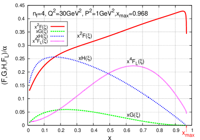
Figure 3: The four functions $F$, $G$, $H$ and $F_{L}$ as functions of $x$. $Q^{2}=30{\rm GeV}^{2}$ and $P^{2}=1{\rm GeV}^{2}$. $x_{\rm max}=0.968$.

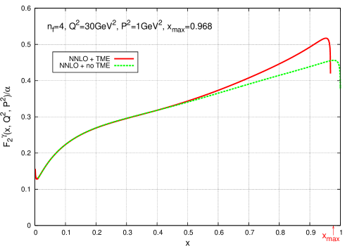
Figure 4: $F_{2}^{\gamma}(x,Q^{2},P^{2})$ as a function of $x$ for $Q^{2}=30{\rm GeV}^{2}$ and $P^{2}=1{\rm GeV}^{2}$ with $x_{\rm max}=0.968$.

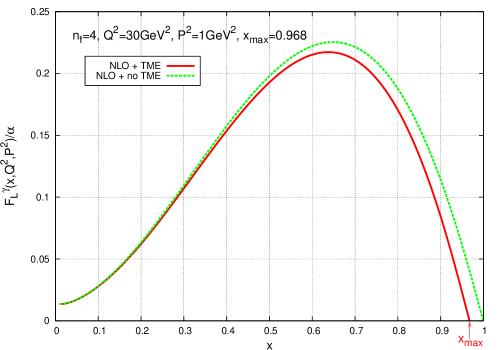
Figure 5: $F_{L}^{\gamma}(x,Q^{2},P^{2})$ as a function of $x$ for $Q^{2}=30{\rm GeV}^{2}$ and $P^{2}=1{\rm GeV}^{2}$ with $x_{\rm max}=0.968$.

One should note that $F(\xi)$ is dominant at larger $x$ region, and determines the leading behavior of $F_{2}^{\gamma}$. And the factor $x^{2}/r^{3}$ in front of $F_{2}^{\gamma}$ shows the deviation upwards from $x^{2}$ as $x$ approaches $x_{\rm max}$. On the other hand, the expression for $F_{L}^{\gamma}$, Eq.(51), possesses no dependence upon the function $F(\xi)$, in contrast to the case of $F_{2}^{\gamma}$. This is a reason why $F_{L}^{\gamma}$ becomes maximum in the middle $x$ region, as seen from Fig.3.

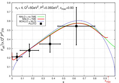
Figure 6: NNLO predictions with and without TME for the effective photon structure function: $F_{\rm eff}^{\gamma}=F_{2}^{\gamma}+\frac{3}{2}F_{L}^{\gamma}$ for $Q^{2}=5{\rm GeV}^{2}$ and $P^{2}=0.35{\rm GeV}^{2}$ with $x_{\rm max}=0.93$. The experimental data are from the PLUTO group PLUTO . The Box diagram prediction to the NLO order is also shown (blue short-dotted line).

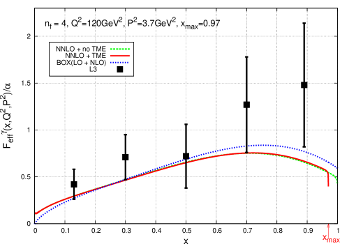
Figure 7: NNLO predictions with and without TME and Box prediction (NLO) on $F_{\rm eff}^{\gamma}=F_{2}^{\gamma}+\frac{3}{2}F_{L}^{\gamma}$ for $Q^{2}=120{\rm GeV}^{2}$ and $P^{2}=3.7{\rm GeV}^{2}$ with $x_{\rm max}=0.970$. The data are from the L3 Group L3 .

Now let us compare our theoretical prediction for the virtual photon structure functions with the existing experimental data. In Fig.6 and Fig.7, we have plotted the experimental data from PLUTO Collaboration PLUTO and also those from L3 Collaboration L3 on the so-called “effective photon structure function”defined as $F_{\rm eff}^{\gamma}=F_{2}^{\gamma}+\frac{3}{2}F_{L}^{\gamma}$, together with the theoretical predictions. The effective structure function is proportional to $\sigma_{TT}+\sigma_{LT}+\sigma_{TL}+\sigma_{LL}$, where $\sigma_{ab}$ ($a,b=T,L$; $T=$ transverse and $L=$ longitudinal) is the total cross section with the helicity state (a) of the probe photon and helicity (b) of the target photon. This combination of $F_{2}^{\gamma}$ and $F_{L}^{\gamma}$ is obtained in the limit of $P^{2}/Q^{2}\ll 1$ GRS ; Nisi ; GRSch .

In the above experiments we have $Q^{2}=5\ (120)\ {\rm GeV}^{2}$ and $P^{2}=0.35\ (3.7)\ {\rm GeV}^{2}$ with $x_{\rm max}=0.93\ (0.97)$, for PLUTO (L3) data. Here we note that for the PLUTO data, $P^{2}\ll Q^{2}$ is satisfied since $P^{2}/Q^{2}\simeq 0.07$, but $P^{2}$ is not much larger than $\Lambda^{2}$ i.e. $\Lambda^{2}/P^{2}\simeq 0.114$. For L3 data, both hierarchical conditions are satisfied. Although the experimental error bars are rather large, the data are considered to be roughly consistent with the theoretical expectations, except for the larger $x$ region in the case of L3 data. Note that the TME for the $F_{\rm eff}^{\gamma}$ in this kinematical region is almost negligible for both cases. This could be explained as a consequence of the cancellation of the TME between $F_{2}^{\gamma}$ and $F_{L}^{\gamma}$, as discussed above.

VI Conclusions

We have investigated the target mass corrections for the unpolarized virtual photon structure functions $F_{2}^{\gamma}(x,Q^{2},P^{2})$ and $F_{L}^{\gamma}(x,Q^{2},P^{2})$ to the NNLO in perturbative QCD.

In contrast to the case of the nucleon target, the virtual photon target provides us with the unique testing ground for the perturbatively calculable target mass effects. Taking into account the trace terms in the operator matrix elements by using the expansion in terms of orthogonal Gegenbauer polynomials we get the Nachtmann moments. These moments were then inverted to derive explicit expressions for $F_{2}^{\gamma}(x,Q^{2},P^{2})$ and $F_{L}^{\gamma}(x,Q^{2},P^{2})$ in terms of the four profile functions which are calculable to NNLO for the first three functions $F$, $G$, $H$ and to NLO for the last one $F_{L}$. The TME becomes sizable at larger $x$ region, and it enlarges $F_{2}^{\gamma}$ near $x_{\rm max}$ and reduces $F_{L}^{\gamma}$ in the region of $x$ larger than the middle point. When we go to higher values of $P^{2}$, e.g. $P^{2}=3{\rm GeV}^{2}$ for $Q^{2}=30{\rm GeV}^{2}$, it has turned out that the $F_{2}^{\gamma}$ blows up as $x$ approaches $x_{\rm max}$. So some prescription like resummation of large logs would be needed to avoid such difficulties.

We have carried out the confrontation of our theoretical predictions with the existing experimental data on the effective photon structure function $F_{\rm eff}^{\gamma}$ from PLUTO and also those from L3 Collaboration. Roughly speaking we find the rather good agreement between theory and experiments. However, it turned out that TME looks almost negligible for $F_{\rm eff}^{\gamma}$, which is the combination of $F_{2}^{\gamma}$ and $F_{L}^{\gamma}$ and exhibits a cancellation of TME between them. In the present analysis, we have treated the active flavors as massless quarks, and ignored the mass effects of the heavy flavors, which should remain as a future subject. We should also investigate the power corrections $(P^{2}/Q^{2})^{k}$ ($k=1,2,\cdots$) due to the higher-twist effects.

We expect the future experiments would provides us with more accurate data for the double-tag two-photon processes in $e^{+}e^{-}$ collisions.

Appendix A Photon Structure functions

Averaging the structure tensor $W_{\mu\nu\rho\tau}(p,q)$ given in Eq.(4) over the target polarization, we get BCG ; SSU

$$W_{\mu\nu}^{\gamma}(p,q) = -\frac{g^{\rho\tau}}{2}W_{\mu\nu\rho\tau}(p,q)$$ (53)

$$= R_{\mu\nu}\Bigl{[}W_{TT}-\frac{1}{2}W_{TL}\Bigr{]}+k_{1{\mu}}k_{1{\nu}}\Bigl{[}W_{LT}-\frac{1}{2}W_{LL}\Bigr{]}~{},$$

where

$$R_{\mu\nu} = -g_{\mu\nu}+\frac{1}{X}\left[p\cdot q\left(q_{\mu}p_{\nu}+p_{\mu}q_{\nu}\right)-q^{2}p_{\mu}p_{\nu}-p^{2}q_{\mu}q_{\nu}\right]$$ (54)

$$k_{1\mu} = \sqrt{\frac{-q^{2}}{X}}\left(p_{\mu}-\frac{p\cdot q}{q^{2}}q_{\mu}\right)$$ (55)

with $X=(p\cdot q)^{2}-q^{2}p^{2}$. In the above equation the first index ($a=T,L$) of the invariant functions $W_{ab}$ refers to the probe photon and the second one ($b=T,L$) to the target photon, and the subscripts $T$ and $L$ denote the transverse and longitudinal photon, respectively.

We define the unpolarized photon structure functions $F_{2}^{\gamma}$ and $F_{L}^{\gamma}$ as,

$$\frac{1}{x}F_{2}^{\gamma} = \frac{(p\cdot q)^{2}}{X}\left\{\Bigl{[}W_{TT}-\frac{1}{2}W_{TL}\Bigr{]}+\Bigl{[}W_{LT}-\frac{1}{2}W_{LL}\Bigr{]}\right\}~{},$$ (56)

$$\frac{1}{x}F_{L}^{\gamma} = W_{LT}-\frac{1}{2}W_{LL}~{}.$$ (57)

Another structure function $F_{1}^{\gamma}$ is often used, which is defined as BergerWagner

$$F_{1}^{\gamma}=W_{TT}-\frac{1}{2}W_{TL}.$$ (58)

Then we get a well-known relation

$$F_{L}^{\gamma}=-xF_{1}^{\gamma}+\frac{X}{(p\cdot q)^{2}}F_{2}^{\gamma}=-xF_{1}^{\gamma}+\left(1-\frac{4x^{2}P^{2}}{Q^{2}}\right)F_{2}^{\gamma}~{}.$$ (59)

Since $R_{\mu\nu}$ and $k_{1{\mu}}k_{1{\nu}}$ are expressed in terms of $e_{\mu\nu}$ and $d_{\mu\nu}$, which are given in Eqs.(7) and (8), as

$$R_{\mu\nu} = \frac{p^{2}q^{2}}{X}e_{\mu\nu}+\frac{(p\cdot q)^{2}}{X}d_{\mu\nu}~{},$$ (60)

$$k_{1{\mu}}k_{1{\nu}} = \frac{(p\cdot q)^{2}}{X}\{e_{\mu\nu}+d_{\mu\nu}\}~{},$$ (61)

we find that $W_{\mu\nu}^{\gamma}(p,q)$ in (53) is rewritten as

$$W_{\mu\nu}^{\gamma}(p,q) = e_{\mu\nu}\left\{\frac{1}{x}F_{L}^{\gamma}+\frac{p^{2}q^{2}}{(p\cdot q)^{2}}\frac{1}{x}F_{2}^{\gamma}\right\}+d_{\mu\nu}\frac{1}{x}F_{2}^{\gamma}~{},$$ (62)

Appendix B Gegenbauer polynomials

The Gegenbauer polynomials are defined through the generating function given by Bateman ; GRAD

$$(1-2\eta t+t^{2})^{-\nu}=\sum_{n=0}^{\infty}C_{n}^{(\nu)}(\eta)t^{n}.$$ (63)

In terms of hypergeometric functions $F(\alpha,\beta,\gamma;\,z)$,   $C_{n}^{(\nu)}(\eta)$ is expressed as

$$C_{n}^{(\nu)}(\eta) = \frac{2^{n}\Gamma(n+\nu)}{n!\Gamma(\nu)}\eta^{n}F\left(-\frac{n}{2},\frac{1-n}{2},1-n-\nu;\frac{1}{\eta^{2}}\right)$$ (64)

$$= \frac{1}{\Gamma(\nu)}\sum_{j=0}^{n/2}\frac{(-1)^{j}\Gamma(\nu+n-j)}{j!(n-2j)!}\,(2\,\eta)^{n-2j}~{}.$$

For example, we have

$$C_{n}^{(1)}(\eta) = \sum_{j=0}^{n/2}\frac{(-1)^{j}}{j!}\frac{(n-j)!}{(n-2j)!}(2\eta)^{n-2j}~{},$$ (65)

B.1 Orthogonality relations

The orthogonality relation reads

$$\int_{-1}^{1}(1-\eta^{2})^{\nu-\frac{1}{2}}C_{m}^{(\nu)}(\eta)C_{n}^{(\nu)}(\eta)d\eta=\frac{2\pi}{2^{2\nu}}\frac{\Gamma(n+2\nu)}{(n+\nu)n![\Gamma(\nu)]^{2}}\delta_{mn}.$$ (66)

In addition we have the following formula for the integral to project out the contributions of definite spin from the dispersion relations,

$$\int_{-1}^{1}d\eta\ \eta^{m}(1-\eta^{2})^{\nu-\frac{1}{2}}C_{n}^{(\nu)}(\eta)\frac{1}{\zeta-\eta}=\frac{\pi}{2^{\nu-1}}\zeta^{m}(\zeta^{2}-1)^{\frac{\nu-1}{2}}\left[\zeta-(\zeta^{2}-1)^{1/2}\right]^{n+\nu}$$

$$\hskip 56.9055pt\times\frac{\Gamma(n+2\nu)}{\Gamma(\nu)\Gamma(n+\nu+1)}F\left(\nu,1-\nu,n+\nu+1;\frac{-\zeta+(\zeta^{2}-1)^{1/2}}{2(\zeta^{2}-1)^{1/2}}\right).$$ (67)

In fact the factor $\left[\zeta-(\zeta^{2}-1)^{1/2}\right]^{n+\nu}$ gives $\left(-\frac{P}{Q}\right)^{n+\nu}~{}\xi^{n+\nu}$, where $\xi$ is the so-called $\xi$-scaling variable given in Eq.(22).

B.2 Recursion relations

The recursion relations for Gegenbauer polynomials read

$$nC_{n}^{(\nu)}(\eta)=2\nu[\eta C_{n-1}^{(\nu+1)}(\eta)-C_{n-2}^{(\nu+1)}(\eta)]~{},$$ (68)

$$(n+2\nu)C_{n}^{(\nu)}(\eta)=2\nu[C_{n}^{(\nu+1)}(\eta)-\eta C_{n-1}^{(\nu+1)}(\eta)]~{},$$ (69)

$$(n+2)C_{n+2}^{(\nu)}(\eta)=2(n+\nu+1)\eta C_{n+1}^{(\nu)}(\eta)-(n+2\nu)C_{n}^{(\nu)}(\eta)~{}.$$ (70)

We get from (68) and (69),

$$C_{n}^{(\nu)}(\eta) = \frac{\nu}{n+\nu}\Bigl{[}C_{n}^{(\nu+1)}(\eta)-C_{n-2}^{(\nu+1)}(\eta)\Bigr{]}$$ (71)

$$C_{n}^{(\nu)}(\eta) = \frac{\nu}{n+\nu}\cdot\frac{\nu+1}{n+\nu+1}C_{n}^{(\nu+2)}(\eta)$$ (72)

$$-\frac{2\nu(\nu+1)}{(n+\nu)^{2}-1}C_{n-2}^{(\nu+2)}(\eta)+\frac{\nu}{n+\nu}\cdot\frac{\nu+1}{n+\nu-1}C_{n-4}^{(\nu+2)}(\eta)$$

Now we derive the second line of Eq.(32). Choosing $\nu=2$ and $n\rightarrow(n-2)$ in (71), we find

$$C_{n-2}^{(2)}(\eta)=\frac{2}{n}\Bigl{[}C_{n-2}^{(3)}(\eta)-C_{n-4}^{(3)}(\eta)\Bigr{]}~{}.$$ (73)

Next choosing $\nu=3$ and $n\rightarrow(n-4)$ in (70), we get

$$4\eta C_{n-3}^{(3)}(\eta)=\frac{2}{n}\left[(n-2)C_{n-2}^{(3)}(\eta)+(n+2)C_{n-4}^{(3)}(\eta)\right]~{}.$$ (74)

Thus we obtain

$$\Bigl{[}C_{n-2}^{(2)}(\eta)-2C_{n-4}^{(3)}(\eta)+4\eta C_{n-3}^{(3)}(\eta)\Bigr{]}-2C_{n-2}^{(3)}(\eta)=\frac{-2}{n}C_{n-2}^{(3)}(\eta)+\frac{2}{n}C_{n-4}^{(3)}(\eta)$$ (75)

Appendix C Contraction Formulas

Here we derive Eqs.(12) and (13). The most general rank-$n$ symmetric and traceless tensor, $\{p^{\mu_{1}}\cdots p^{\mu_{n}}\}_{n}$, that can be formed with the momentum $p$ alone, is expressed as follows GP ,

$$\{p^{\mu_{1}}\cdots p^{\mu_{n}}\}_{n}=\sum_{j=0}^{n/2}\frac{(-1)^{j}}{2^{j}}\frac{(n-j)!}{n!}\underbrace{g\cdots g}_{j}\overbrace{p\cdots p}^{n-2j}~{}(p^{2})^{j}~{},$$ (76)

where $\displaystyle{\underbrace{g\cdots g}_{j}}$ stands for a product of $j$ metric tensors $g^{\mu_{l}\mu_{k}}$ with $2j$ indices chosen among $\mu_{1},\cdots,\mu_{n}$ in all possible ways. Then we easily see that the contraction of $\{p^{\mu_{1}}\cdots p^{\mu_{n}}\}_{n}$ with $q_{\mu_{1}}\cdots q_{\mu_{n}}$ is expressed in terms of Gegenbauer polynomial $C_{n}^{(1)}(\eta)$ given in (65) as NACHT ; WAND ,

$$q_{\mu_{1}}\cdots q_{\mu_{n}}\{p^{\mu_{1}}\cdots p^{\mu_{n}}\}=a^{n}C_{n}^{(1)}(\eta)~{},$$ (77)

which is Eq.(12). Here we have put

$$a=-\frac{1}{2}PQ,\quad\eta=-\frac{p\cdot q}{PQ}~{}.$$ (78)

Next we differentiate both sides of Eq.(77) twice with respect to $q_{\alpha}$ and $q_{\beta}$. The left-hand side becomes

$$\frac{\partial}{\partial q_{\alpha}}\frac{\partial}{\partial q_{\beta}}\Bigl{(}q_{\mu_{1}}\cdots q_{\mu_{n}}\{p^{\mu_{1}}\cdots p^{\mu_{n}}\}_{n}\Bigr{)}=n(n-1)q_{\mu_{1}}\cdots q_{\mu_{n-2}}\{p^{\alpha}p^{\beta}p^{\mu_{1}}\cdots p^{\mu_{n-2}}\}_{n}~{}.$$ (79)

Differentiation of $a^{n}C_{n}^{(1)}(\eta)$ with respect to $q_{\alpha}$ gives

$$\frac{\partial}{\partial q_{\alpha}}\left(a^{n}C_{n}^{(1)}(\eta)\right)=na^{n-1}\left(\frac{-aq^{\alpha}}{Q^{2}}\right)C_{n}^{(1)}(\eta)+a^{n}\cdot 2C_{n-1}^{(2)}(\eta)\left(\frac{p^{\alpha}}{2a}+\eta\frac{q^{\alpha}}{Q^{2}}\right)$$

$$\hskip 85.35826pt=\frac{q^{\alpha}}{Q^{2}}a^{n}~{}2C_{n-2}^{(2)}(\eta)+p^{\alpha}a^{n-1}C_{n-1}^{(2)}(\eta)$$ (80)

where we have used the following formulas

$$\frac{\partial a}{\partial q_{\alpha}}=a~{}\Bigl{(}\frac{-q^{\alpha}}{Q^{2}}\Bigr{)}~{},\qquad\frac{\partial\eta}{\partial q_{\alpha}}=\frac{p^{\alpha}}{2a}+\eta\frac{q^{\alpha}}{Q^{2}},\qquad\frac{dC_{n}^{(\nu)}(\eta)}{d\eta}=2\nu C_{n-1}^{(\nu+1)}(\eta)~{},$$ (81)

and, at the last line, the recursion relation (68). Further, we differentiate the both sides of Eq.(80) with respect to $q_{\beta}$ . Again using the formulas in (81) and the recursion relation (68), we get

$$\frac{\partial}{\partial q_{\alpha}}\frac{\partial}{\partial q_{\beta}}\left(a^{n}C_{n}^{(1)}(\eta)\right)=\frac{g^{\alpha\beta}}{Q^{2}}a^{n}\cdot 2C_{n-2}^{(2)}(\eta)+\frac{q^{\alpha}q^{\beta}}{Q^{4}}a^{n}\cdot 8C_{n-4}^{(3)}(\eta)$$

$$\hskip 85.35826pt+p^{\alpha}p^{\beta}a^{n-2}\cdot 2C_{n-2}^{(3)}(\eta)+\frac{p^{\alpha}q^{\beta}+q^{\alpha}p^{\beta}}{Q^{2}}a^{n-1}\cdot 4C_{n-3}^{(3)}(\eta)$$ (82)

Thus, from Eqs.(79) and (82), we obtain

$$q_{\mu_{1}}\cdots q_{\mu_{n-2}}\{p^{\alpha}p^{\beta}p^{\mu_{1}}\cdots p^{\mu_{n-2}}\}_{n}$$

$$\qquad=\frac{1}{n(n-1)}\left[\frac{g^{\alpha\beta}}{Q^{2}}a^{n}\cdot 2C_{n-2}^{(2)}(\eta)+\frac{q^{\alpha}q^{\beta}}{Q^{4}}a^{n}\cdot 8C_{n-4}^{(3)}(\eta)\right.$$

$$\qquad\quad\left.+p^{\alpha}p^{\beta}a^{n-2}\cdot 2C_{n-2}^{(3)}(\eta)+\frac{p^{\alpha}q^{\beta}+q^{\alpha}p^{\beta}}{Q^{2}}a^{n-1}\cdot 4C_{n-3}^{(3)}(\eta)\right]~{},$$ (83)

which is Eq.(13).

Appendix D Nachtmann moments of $F_{L}^{\gamma}$

By applying the orthogonality relation (66) for $\nu=3$ to the longitudinal amplitude (32) with the help of (33) we derive the following recursive relation for $M_{L,n}^{\gamma}$’s:

$$M_{L,n}^{\gamma}-2\kappa\frac{n+1}{n+4}M_{L,n+2}^{\gamma}+\kappa^{2}\frac{(n+1)(n+2)}{(n+4)(n+5)}M_{L,n+4}^{\gamma}=I_{n}~{},$$ (84)

where

$$I_{n}=\int_{0}^{x_{\rm max}}\frac{dx}{x^{5}}\xi^{n+3}\left[\frac{3+3(n+3)r+(n+2)(n+4)r^{2}}{(n+4)(n+5)}\right]F_{L}^{\gamma}(x,Q^{2},P^{2})$$

$$\hskip 85.35826pt+4\kappa\frac{1}{n+2}M_{2,n+2}^{\gamma}-4\kappa^{2}\frac{(n+1)(n+2)}{(n+3)(n+4)^{2}}M_{2,n+4}^{\gamma}~{}.$$ (85)

The above recursive equation (84) can be solved as an infinite series:

$$M_{L,n}^{\gamma}=(n+1)\sum_{l=0}^{\infty}\kappa^{l}\frac{(l+1)(n+2+l)}{(n+2l+1)(n+2l+2)}I_{n+2l}~{}.$$ (86)

Introducing a variable $t$ defined by ${\xi}(P/Q)\equiv t$ we have

$$\xi\sqrt{\kappa}=t,\quad r=\frac{1-t^{2}}{1+t^{2}},\quad\kappa\xi x=\frac{t^{2}}{1+t^{2}},\quad\int_{0}^{x_{\rm max}}dx\ [\ \cdots]=\int_{0}^{1}d\xi\frac{1-t^{2}}{(1+t^{2})^{2}}\ [\ \cdots]~{},$$ (87)

and then in terms of $t$ we can sum up the above infinite series and find

$$M_{L,n}^{\gamma}=\int_{0}^{1}d\xi\ \xi^{n}\frac{1-t^{2}}{1+t^{2}}\left[\frac{1}{x^{2}}F_{L}^{\gamma}(x,Q^{2},P^{2})+4\kappa\frac{(n+3)-(n+1)t^{2}}{(n+2)(n+3)}F_{2}^{\gamma}(x,Q^{2},P^{2})\right]~{},$$ (88)

the right-hand side of which turns out to be the Nachtmann moments (21), $\mu_{L,n}^{\gamma}$.

References

(1) T.F. Walsh, Phys. Lett.36B, 121 (1971);
S.J. Brodsky, T. Kinoshita and H. Terazawa, Phys. Rev. Lett.27, 280 (1971).
(9)
M. Stratmann and W. Vogelsang, Phys. Lett.B386, 370 (1996).
(10)
M. Glück, E. Reya and C. Sieg, Phys. Lett.B503, 285 (2001);
Eur. Phys. J.C20, 271 (2001).
(11)
T. Uematsu and T. F. Walsh, Phys. Lett.101B, 263 (1981).
(12)
T. Uematsu and T. F. Walsh, Nucl. Phys.B199, 93 (1982).
(13)
G. Rossi, Phys. Rev.D29, 852 (1984).
(14)
M. Drees and R. M. Godbole, Phys. Rev.D50, 3124 (1994).
(15)
M. Glück, E. Reya and M. Stratmann, Phys. Rev.D51, 3220 (1995); Phys. Rev.D54, 5515 (1996).
(16)
M. Fontannaz, Eur. Phys. C20, 297 (2004).
(17)
K. Sasaki and T. Uematsu, Phys. Rev.D59, 114011 (1999).
(18)
K. Sasaki and T. Uematsu,
Phys. Lett.B473, 309 (2000); Eur. Phys. J.C20, 283 (2001).
(19)
K. Sasaki, T. Ueda and T. Uematsu,
Phys. Rev.D73, 094024 (2006).
(20)M. Krawczyk,
AIP Conf. Proc. No.571 (AIP, New York, 2001) and
references therein;
M. Krawczyk, A. Zembrzuski and M. Staszel,
Phys. Rep.345, 265 (2001);
R. Nisius, Phys. Rep.332, 165 (2001); hep-ex/0110078;
M. Klasen,
Rev. Mod. Phys.74, 1221 (2002);
I. Schienbein,
Ann. Phys.301, 128 (2002);
R. M. Godbole,
Nucl. Phys. B (Proc. Suppl.) 126, 414 (2004).
(21)
T. Ueda, K. Sasaki and T. Uematsu,
Phys. Rev.D75, 114009 (2007).
(22)
S. Moch, J.A.M. Vermaseren and A. Vogt, Nucl. Phys.B688, 101 (2004).
(23)
A. Vogt, S. Moch and J.A.M. Vermaseren, Nucl. Phys.B691, 129 (2004).
(24)
A. Vogt, S. Moch and J.A.M. Vermaseren, Acta Phys. PolonB37, 683 (2006);
hep-ph/0511112.
(25)
O. Nachtmann, Nucl. Phys.B63, 237 (1973);
B78, 455 (1974).
(26)
H. Georgi and H. Politzer, Phys. Rev.D14, 1829 (1976).
(27)
A. De Rujula, H. Georgi and H. Politzer, Ann. of Phys.103, 315 (1977); Phys. Rev.D15, 2495 (1977).
(28)
S. Wandzura, Nucl. Phys.B122, 412 (1977).
(29)
S. Matsuda and T. Uematsu, Nucl. Phys.B168, 181 (1980).
(30)
H. Kawamura and T. Uematsu, Phys. Lett.B343, 346 (1995).
(31)
A. Piccione and G. Ridolfi, Nucl. Phys.B513, 301 (1998).
(32)
J. Blümlein and A. Tkabladze, Nucl. Phys.B553, 427
(1999).
(33)
H. Baba, K. Sasaki and T. Uematsu, Phys. Rev.D65, 114018
(2002).
(34)
S. Simula, Phys. Lett.B574, 189 (2003).
(35)
F. M. Steffens and W. Melnitchouk, Phys. Rev.C73, 055202
(2006).
(36) For a recent review, see for example, I. Schienbein et al.,
arXiv:0709.1775 [hep-ph] .