The spectrum of charmed mesons from dynamical anisotropic lattices

Abstract

We present our preliminary analysis for the chamonium and D_s spectra obtained from N${}_{f}=2$ dynamical anisotropic lattices. We use 12${}^{3}\times 80$ lattices with lattice spacing $a_{t}=7.35$ GeV^-1 and anisotropy of six. Meson correlators are computed using all-to-all propagators together with variational analysis.

I INTRODUCTION

In recent years, there has been renewed interest in charm physics. Many new states such as the X(3872), the Y(4260) and the $D_{sJ}$ have been observed Choi:2003ue ; Aubert:2005rm ; Abe:2004zs ; Aubert:2003fg ; Besson:2003jp and their precise measurement including $J^{PC}$ numbers, has become an important topic both experimentally and theoretically.

In principle, lattice QCD should be able to answer these questions from first principles but it requires high precision numerical simulations. In this region of the quark mass relativistic effects could be important. However, simulations of the charm quark with isotropic lattices are expensive. In this study we use a relativistic anisotropic lattice formulation with $N_{f}=2$ dynamical quarks to study charmonium and $D_{s}$ spectra. In this formulation, the lattice is discretized along the spatial, $a_{s}$, and temporal, $a_{t}$, directions with $\xi=a_{s}/a_{t}\gg 1$. Anisotropic lattices have the advantage of having small discretization errors in the temporal direction whilst keeping the computational cost down. In addition, keeping a small temporal lattice spacing allows us to increase the number of time slices which in turn makes it easier to identify the plateau regions in effective mass plots. It is difficult to achieve this using isotropic lattices since the heavy hadron correlators with a charm or bottom quark have a signal that decays rapidly. Our aim is to be able to extract the excited spectra with small statistical errors.

Our lattice actions are described in section II. In section III we summarize the parameters and the interpolating operators used in the simulation. In section IV we discuss the method to obtain excited spectra. In conclusion, we discuss our results and future plans.

II ANISOTROPIC ACTIONS

In this section, we describe the gauge and quark actions used in the simulation. The gauge action is a Two-Plaquette Symanzik-improved action which is designed to study glueballs Morningstar:1999dh . It is given by

$$S_{G} = \frac{\beta}{\xi_{g}^{0}}\left\{\frac{5(1+w)}{3u_{s}^{4}}\Omega_{s}-\frac{5w}{3u_{S}^{8}}\Omega_{s}^{(2t)}-\frac{1}{12u_{s}^{6}}\Omega_{s}^{R}\right\}$$ (1)

$$+ \beta\xi_{g}^{0}\left\{\frac{4}{3u_{s}^{2}u_{t}^{2}}\Omega_{t}-\frac{1}{12u_{s}^{4}u_{t}^{2}}\Omega_{t}^{(R)}\right\},$$

where $\Omega_{s}$ and $\Omega_{t}$ are the spatial and temporal plaquettes respectively. $\Omega_{s}^{(R)}$ and $\Omega_{t}^{(R)}$ refer to space-space and space-time rectangles and $\Omega_{s}^{(2t)}=\frac{1}{2}\sum_{x,i>j}\left[1-P_{ij}(x)P_{ij}(x+\hat{t})\right]$. This action has leading discretization errors of $O(a_{s}^{4},a_{t}^{2},\alpha_{s}a_{s}^{2})$.

The $O(a_{s}^{3},a_{t},\alpha_{s}a_{s})$-improved anisotropic quark action Foley:2004jf is given by

$$S_{q} = \bar{\psi}\left[\gamma_{0}\nabla_{0}+\sum_{i}\mu_{r}\gamma_{i}\nabla_{i}\left(1-\frac{1}{\xi_{q}^{0}a_{s}^{2}}\Delta_{i}\right)\right.$$ (2)

$$- \left.\frac{ra_{t}}{2}\Delta_{i0}+sa_{s}^{3}\sum_{i}\Delta_{i}^{2}+m_{0}\right]\psi,$$

where $r$ and $s$ are the Wilson parameters and $\mu_{r}=(1+ra_{t}m_{0}/2)$. The derivatives are defined as

$$\nabla_{\mu}\psi(x)=\frac{1}{2a_{\mu}}\left[U_{\mu}(x)\psi(x\!+\!\hat{\mu})-U_{\mu}^{\dagger}(x\!-\!\hat{\mu})\psi(x\!-\!\hat{\mu})\right],$$ (3)

$$\Delta_{\mu}\psi(x) = \frac{1}{a_{\mu}^{2}}\left[U_{\mu}(x)\psi(x\!+\!\hat{\mu})\!+\!U_{\mu}^{\dagger}(x-\hat{\mu})\psi(x\!-\!\hat{\mu})\right.$$ (4)

$$-\!\left.2\psi(x)\right],$$

and $\xi_{q}^{0}$ is the bare quark anisotropy. In order to maximize the plaquette stout links Morningstar:2003gk are used. We used the same quark action to simulate light sea quarks and heavy valence quarks. Our sea quark mass in this simulation is close to the strange quark mass.

The ratio of the lattice spacings, $a_{s}/a_{t}$, which appears in both the gauge and the quark actions, as $\xi_{g}^{0}$ and $\xi_{q}^{0}$ respectively, are bare parameters that need to be tuned. In a quenched study, this tuning can be done separately. However, sea quark effects in dynamical simulations lead to a simultaneous non-trivial tuning of the anisotropies. This procedure is explained in detail in Ref. Morrin:2005tc . For the results presented in these proceeding the renormalized anisotropy, $\xi_{r}$ is set to be 6.

III SIMULATION DETAILS

In this study, we obtained the charmonium and the $D_{s}$ spectra from $12^{3}\times 80$ lattices with 250 configurations. We tuned the valence charm quark mass to $a_{t}m_{c}=0.117$ in order to get the $J/\psi$ mass correct while the light quark mass is $a_{t}m_{sea}=a_{t}m_{light}=-0.057$ which is close to the strange quark mass. We use the all-to-all propagator method with “dilution” of Ref. Foley:2005ac with no eigenvalues for the charm quark propagators and 20 eigenvalues for the strange quark propagators. We used time, space(even/odd) and color dilution for the charmonium study while color dilution is omitted in the $D_{s}$ case. The lattice spacing is set from the spin-averaged (1P-1S) splitting in the charmonium system and found to be $a_{t}\simeq 0.0272$ fm. The parameters used are listed in table 1.

11.5

Table 1: Simulation parameters.

Configurations	250 ($a_{t}m_{c}=0.117$,
	$a_{t}m_{sea}=a_{t}m_{light}=-0.057$)
Dilution	time, space(even/odd), color ($\bar{c}c$)
	time, space(even/odd) , ($D_{s}$)
Physics	S, P and D waves, hybrids
Volume	$12^{3}\times 80$
$N_{f}$	2
$a_{s}$	$\sim 0.17$ fm
$a_{t}^{-1}$	$7.35\pm 0.03$ GeV

Taking advantage of the all-to-all propagators, we use a variational method Luscher:1990ck ; Michael:1985ne in order to get a better overlap with higher excited states where we use a spatially extended operator basis Lacock:1996vy . The lattice operators used in this study along with their putative continuum spin assignments are given in table 2. We have assumed the simplest possible continuum assignment is correct. The validity of this assumption is under investigation. Using the operator basis in table 2, for a given channel $R$ one can construct the matrix

$$C^{(R)}_{\alpha\beta}(t)=\langle 0|O^{(R)}_{\alpha}(t)O^{\dagger(R)}_{\beta}(0)|0\rangle,$$ (5)

where $\alpha,\beta=1,\dots,n$ represent the different interpolating operators, constructed by applying different levels of quark smearing. The different energy levels can then be obtained from

$$\lim_{t\rightarrow\infty}\lambda_{\alpha}(t,t_{0})=e^{-(t-t_{0})E_{\alpha}}\left[1+O(e^{-t\Delta E_{\alpha}})\right],$$ (6)

where $\lambda_{\alpha}$ are the eigenvalues of the matrix $C(t_{0})^{-1/2}C(t)C(t_{0})^{-1/2}$ and $t_{0}$ is some small reference time. We performed single state fits to the diagonal elements in order to extract the ground and excited states.

Table 2: The operator basis used to obtain the $\bar{c}c$ and $D_{s}$ spectra. Definitions of the $s_{i},p_{i}$ and $t_{i}$ are given in Ref. Lacock:1996vy .

$J^{\rm PC}$	${}^{2S+1}L_{J}$	STATE	OPERATORS
$0^{-+}$	${}^{1}S_{0}$	$\eta_{c}$,$\eta_{c}^{{}^{\prime}}$	$\gamma_{5}$,$\gamma_{5}\sum_{i}s_{i}$
$1^{--}$	${}^{3}S_{1}$	J/$\psi$,$\psi$(2S)	$\gamma_{j}$,$\gamma_{j}\sum_{i}s_{i}$
$1^{+-}$	${}^{1}P_{1}$	$h_{c}$,$h_{c}^{{}^{\prime}}$	$\gamma_{i}\gamma_{j}$, $\gamma_{5}p_{j}$
$0^{++}$	${}^{3}P_{0}$	$\chi_{c_{0}}$,$\chi^{{}^{\prime}}_{c_{0}}$	1,$\vec{\gamma}\cdot\vec{p}$
$1^{++}$	${}^{3}P_{1}$	$\chi_{c_{1}}$,$\chi^{{}^{\prime}}_{c_{1}}$	$\gamma_{5}\gamma_{i}$,$\vec{\gamma}\times\vec{p}$
$2^{++}$	${}^{3}P_{2}$	$\chi_{c_{2}}$,$\chi^{{}^{\prime}}_{c_{2}}$	$\vec{\gamma}\times\vec{p}$, $\gamma_{1}p_{1}\!-\!\gamma_{2}p_{2}$
			$2\gamma_{3}p_{3}-\gamma_{1}p_{1}-\gamma_{2}p_{2}$
$2^{-+}$	${}^{1}D_{2}$	$1{}^{1}D_{2}$	$\gamma_{5}(s_{1}-s_{2})$,$\gamma_{5}(2s_{3}-s_{1}-s_{2})$
$2^{--}$	${}^{3}D_{2}$	$1{}^{3}D_{2}$	$\gamma_{j}(s_{i}-s_{k})$,$\gamma_{1}t_{1}-\gamma_{2}t_{2}$,
			$2\gamma_{3}t_{3}-\gamma_{1}t_{1}-\gamma_{2}t_{2}$
$3^{--}$	${}^{3}D_{3}$	$1{}^{3}D_{3}$	$\vec{\gamma}\cdot\vec{t}$
$1^{-+}$	Hybrid	$q\bar{q}g$	$\vec{\gamma}\times\vec{u}$

IV ANALYSIS

Time diluted all-to-all propagators introduce random noise at each time slice which makes it difficult to indentify a plateau region in the effective mass plots which fluctuate more than point-to-all propagators. However, we fit the correlators and a better picture can be obtained from “sliding window” plots (or $t_{min}$ plots). For a fixed value of some $t_{max}$, we vary the $t_{min}$ value and plot the fitted mass. This is illustrated in Figs. 1 and  2 for the $J/\psi$ and $D_{s}$ $0^{-}$ and $1^{-}$ states, respectively Juge:2005nr ; Juge:2006fm .

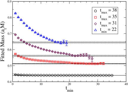
Figure 1: Sliding window plots for the $J/\psi$ obtained from the variational analysis. The plot shows the ground state in the lattice $T_{1_{u}}^{-}$ irreducible representation which corresponds to the continuum $J=1$ state. The higher lying states determined in this channel are assumed to be radial excitations of the $J/\Psi$. This is under investigation.

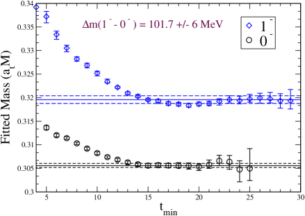
Figure 2: Sliding window plot for the $D_{s}$ $0^{-}$ and $1^{-}$ states. The corresponding experimental value of the $1^{-}-0^{-}$ splitting is 143.8MeV.

We choose our fits based on the $\chi^{2}/N_{df}$ ($<$2), fit range (where the fits are stable) and the fit quality (Q$>$0.2). These values are chosen from our earlier simluations with smaller lattices. Most of our results have better $\chi^{2}$ and $Q$ values.

We performed the same analysis for the $\bar{c}c$ and $D_{s}$ systems. Our preliminary spectra are shown in figures 3 and 4.

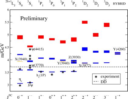
Figure 3: Preliminary charmonium spectrum for the S, P, D waves and the hybrid $1^{-+}$. The results of this study are the blue and red bands. The highest lying radial excitations identified in each channel are coloured red to indicate that these are not free of further excited-state contamination.

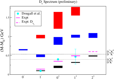
Figure 4: Preliminary $D_{s}$ spectrum for the S and P waves. The results of this study are shown by the blue and red bands. As in the charmonium case the highest lying radial excitations identified in each channel are coloured red to indicate that these are not free of further excited-state contamination. The blue dots represent the UKQCD ($N_{f}=2$) results Dougall:2003hv .

V Conclusions and Outlook

We have presented our preliminary results for the charmonium and $D_{s}$ systems from $N_{f}=2$ dynamical anisotropic lattices. All-to-all propagators are essential in this study and allow us to use a wide range of operators and the variational analysis. For the charmonium system we have good signals for the S, P and D waves and the $1^{-+}$ hybrid. We are planning to expand the simulation to include the $1^{--}$ D-waves and other hybrids. We found the hyperfine splitting in this system to be small. The effect of the chromomagnetic term, $c_{B}{\mathbf{\Sigma}}\cdot{\mathbf{B}}$, disconnected diagrams and stout link smearing are being investigated as possible reasons for this. The $D_{s}$ system is simulated with a low level of dilution. A simulation with a higher level of dilution for this system, with a wider range of operators, is being performed. Both simulations are performed at single lattice spacing where the sea quark mass is around the strange quark mass. Simulations with finer lattices spacings are currently under investigation. The results clearly demonstrate the power of the all-to-all propagators combined with a variational analysis. We have extracted a large number of orbital and radial excitations in the charmonium and $D_{s}$ systems. Further work is also underway to address the continuum spin-identification of these lattice determinations.

- (1) S. K. Choi et al. [Belle Collaboration], Phys. Rev. Lett. 91, 262001 (2003) [arXiv:hep-ex/0309032].
- (2) B. Aubert et al. [BABAR Collaboration], Phys. Rev. Lett. 95, 142001 (2005) [arXiv:hep-ex/0506081].
- (3) K. Abe et al. [Belle Collaboration], Phys. Rev. Lett. 94, 182002 (2005) [arXiv:hep-ex/0408126].
- (4) B. Aubert et al. [BABAR Collaboration],, Phys. Rev. Lett. 90, 242001 (2003) [arXiv:hep-ex/0304021].
- (5) D. Besson et al. [CLEO Collaboration], AIP Conf. Proc. 698, 497 (2004) [arXiv:hep-ex/0305017].
- (6) C. Morningstar and M. J. Peardon, Nucl. Phys. Proc. Suppl. 83, 887 (2000) [arXiv:hep-lat/9911003].
- (7) C. Morningstar and M. J. Peardon, Phys. Rev. D 69, 054501 (2004) [arXiv:hep-lat/0311018].
- (8) J. Foley, A. O’Cais, M. Peardon and S. M. Ryan [TrinLat Collaboration], Phys. Rev. D 73, 014514 (2006) [arXiv:hep-lat/0405030].
- (9) R. Morrin, M. Peardon and S. M. Ryan, PoS LAT2005, 236 (2006) [arXiv:hep-lat/0510016].
- (10) J. Foley, K. Jimmy Juge, A. O’Cais, M. Peardon, S. M. Ryan and J. I. Skullerud, Comput. Phys. Commun. 172, 145 (2005) [arXiv:hep-lat/0505023].
- (11) M. Luscher and U. Wolff, Nucl. Phys. B 339, 222 (1990).
- (12) C. Michael, Nucl. Phys. B 259, 58 (1985).
- (13) P. Lacock, C. Michael, P. Boyle and P. Rowland [UKQCD Collaboration], Phys. Rev. D 54, 6997 (1996) [arXiv:hep-lat/9605025].
- (14) K. J. Juge, A. O’Cais, M. B. Oktay, M. J. Peardon and S. M. Ryan, PoS LAT2005, 029 (2006) [arXiv:hep-lat/0510060].
- (15) K. J. Juge, A. O. Cais, M. B. Oktay, M. J. Peardon, S. M. Ryan and J. I. Skullerud, PoS LAT2006, 193 (2006) [arXiv:hep-lat/0610124].
- (16) A. Dougall, R. D. Kenway, C. M. Maynard and C. McNeile [UKQCD Collaboration], Phys. Lett. B 569, 41 (2003) [arXiv:hep-lat/0307001].